Unified point-edgelet feature tracking
|
|
|
- Regina Blake
- 5 years ago
- Views:
Transcription

1 Clemson University TigerPrints All Theses Theses Unified point-edgelet feature tracking Kalaivani Sundararajan Clemson University, Follow this and additional works at: Part of the Electrical and Computer Engineering Commons Recommended Citation Sundararajan, Kalaivani, "Unified point-edgelet feature tracking" (2011). All Theses This Thesis is brought to you for free and open access by the Theses at TigerPrints. It has been accepted for inclusion in All Theses by an authorized administrator of TigerPrints. For more information, please contact
2 Unified point-edgelet feature tracking A Thesis Presented to the Graduate School of Clemson University In Partial Fulfillment of the Requirements for the Degree Master of Science Electrical Engineering by Kalaivani Sundararajan May 2011 Accepted by: Dr. Stan Birchfield, Committee Chair Dr. Robert Schalkoff Dr. John Gowdy
3 Abstract Feature tracking algorithms have conventionally tracked corner features or windows with high spatial frequency content. However, this conventional point feature representation of scenes would be inappropriate for poorly textured image sequences like indoor image sequences. To overcome this problem, we propose a feature tracking algorithm which tracks point features and edgelets simultaneously. Edgelets are straight line approximations of intensity edges in an image. Hence, a combination of point features and edgelets provides a better representation of untextured sequences with the point features and edgelets complementing each other. We show that this property results in more robust tracking. Tracking edgelets is challenging due to the inherent aperture problem. This thesis proposes an optical flow-based tracking method to track both point features and edgelets in a combined fashion. The aperture problem of the edgelets is overcome using Horn-Schunck regularisation to penalize flow vector deviations from those of the neighboring features. This method uses a translational motion model for tracking individual features and hence only the change in displacement of the point features and edgelets is computed. The point features are detected using the Shi-Tomasi method. The edgelets are detected using the Canny edge map and Douglas-Peucker polyline approximation algorithm. It is assumed that motion will be constant in a neighborhood around the point feature and for all edgels in an edgelet. The point features and edgelets are tracked by minimizing an energy function consisting of the optical flow constraint and sum of negative gradient magnitude of edgels. Thus the edgelets which are typically attracted to the nearby intensity edges will be guided by the optical flow constraint equation and by the motion of the neighboring features. We have also implemented a pyramidal implementation of our algorithm with the uppermost pyramidal level representing the original image and the lower pyramidal levels consisting of the ii
4 downsampled images. The unified feature tracking method utilizes a pyramidal implementation which respects the scale at which the features are visible. Hence, the motion vector computation at lower pyramidal levels is reliable and improves the tracking robustness. Moreover, the average flow vector due to the neighboring features is computed by fitting an affine motion model to the neighboring features. The neighboring features are weighted based on their distance from the feature and the pyramidal level at which they are visible. iii
5 Dedication I dedicate this thesis to my parents, Gowri, Mekhala and Ganesh who have been a great support throughout. iv
6 Acknowledgments I would like to thank my advisor, Dr. Stan Birchfield, for his valuable guidance and insight which made this thesis possible. He has been really supportive, encouraging and inspiring. I would also like to thank Dr.Robert Schalkoff and Dr.John Gowdy for being part of my committee and for their helpful suggestions. Special thanks to Vidya Murali and all students in our research group for their support during the research. I would also like to acknowledge the immense support and encouragement given by all friends and colleagues at Soliton Technologies. Finally, I am thankful to all my friends for their support. v
7 Table of Contents Title Page Abstract i ii Dedication iv Acknowledgments v List of Tables vii List of Figures viii 1 Introduction Tracking primitive features Why a combination of primitive features? Unified feature tracking and its applications Thesis outline Related Work Approach - Unified point-edgelet feature tracking Optical flow and aperture problem Joint tracking of features and edges Unified point-edgelet feature tracking Results Comparison with ground truth and other methods Dense feature representation Computation time Indoor image sequences Effect of scale in tracking Conclusions and Discussion Appendices A Derivation: Unified point-edgelet tracking Bibliography vi
8 List of Tables 4.1 Average Endpoint error and average angular error vii
9 List of Figures 1.1 Different feature representations of an untextured image Unified point-edgelet feature tracking - An overview Edgelet detection Scale space feature detection Results of different feature tracking methods for Dimetrodon and Rubberwhale Results of different feature tracking methods for Venus and Hallway Results of different feature tracking methods for Urban2 and Urban Error at motion discontinuity Average endpoint and angular error for dense optical flow Dense feature representation for the Rubberwhale sequence Computation time for different feature tracking methods Unified point-edgelet feature tracking on Hallway sequence Unified point-edgelet feature tracking on BoBoT sequence C Effect of scale space tracking viii
10 Chapter 1 Introduction Feature tracking methods track different low-level features and involve minimization of an energy function pertaining to the feature attributes. Feature tracking can be used to track a target object in an image sequence and finds its application in object recognition, surveillance and human computer interaction. These applications require detection of object motion in an image sequence. Feature tracking methods are also useful for applications like 3D reconstruction, augmented reality and SLAM. These applications require feature correspondences between image frames to determine the scene geometry and camera motion. Feature tracking methods use different types of primitive features like points, lines, and contours to represent the target. However, a single feature type may not efficiently represent the image content and a combination of different feature types would provide a better representation. 1.1 Tracking primitive features The features are chosen such that they provide a good representation of the target. Conventionally, textured images are represented using point features, man-made environments using lines, and deformable objects using contours. The feature tracking methods depends on the features used for tracking and the features themselves are chosen based on the application. Point features are used to represent textured portions in an image with two-dimensional intensity changes. These point features are typically corners, points of occlusion, discontinuities, or regions of curvature maxima. The point features are detected using corner detectors like Harris 1
11 corner detector [12] or Shi-Tomasi method [23]. These features have sufficient information in their local neighborhood to enable localization and hence can be tracked reliably. Point feature trackers include optical flow based methods like Kanade-Lucas-Tomasi (KLT) feature tracker [25] and its variations [1]. Lines and contour features are used to represent edges with one-dimensional intensity changes. Various edge detectors exist which detect edges as maxima of first order derivatives [6] or zero-crossings of second-order derivatives of image intensities. Tracking edges has been very limited due to the inherent aperture problem. Edges can be localized only in one dimension and hence we can obtain only the motion perpendicular to the edge. Line features are typically tracked by one dimensional search in the direction of edge gradient. For many applications, this method of tracking works reasonably well if the scene is uncluttered and displacement between frames is incremental. Contour features represent edges with arbitrary curvature and are used to represent object boundaries. These features are used when the object shape undergoes deformation in subsequent frames. Contour tracking methods include snakes [15, 14] and level sets [18, 7, 19]. Snakes can track open and closed contours but require initialization very close to the actual edge. Level sets based tracking is used to track only closed contours and does not require initialization very close to the edge. 1.2 Why a combination of primitive features? A combination of primitive features often provides a better representation of the image content. Each primitive feature has its own distinctive property and hence a fusion of different features provides a rich description of the image. Moreover a single primitive feature might not work well under all conditions and hence a fusion of multiple primitive features proves to be more robust. This thesis proposes a combination of point features and edgelets for tracking. Edgelets are straight line approximations of intensity edges in an image. Point features represent textured regions in an image, can be localized easily, and can be tracked reliably. They provide a compact representation of informative regions in an image. Both motion vector components of point features can be computed reliably. However, the presence of such textured regions in an untextured environment is limited and hence the sparse representation using point features is a poor geometric representation of the scene content. Moreover, the point features 2

12 (a) Point feature representation (b) Edgelet representation (c) Combination of point features and edgelets Figure 1.1: Different feature representations of an untextured image are described by their local neighborhood and may undergo substantial change over multiple frames due to change in camera position. In contrast, edgelets prove to be more useful to represent images with poor texture. Image sequences of man-made environments will have more edgelets than point features. They also provide a better insight into the geometric structure of the scene content. Edgelets are represented by one-dimensional intensity change and can be quite robust to lighting and scale changes and to motion blur. However, the invariance to all these conditions also makes them less discriminative. Moreover, when the scene is cluttered or textured, edgelets may not provide a good scene representation. Tracking edgelets under such conditions proves to be difficult due to the ambiguity in edgelet correspondences. Moreover, edgelets can be tracked reliably only in the direction of edgelet gradient and not in the direction perpendicular to the edgelet gradient. Hence, both the point features and edgelets provide complementary information about a scene. Point features are distinctive and but undergo changes with viewpoint, while edgelets are robust to viewpoint changes but lack discrimination. Hence a combination of both edgelets and point features provide a much better representation of the scene. Tracking a combination of both these features proves to be more robust and informative regardless of whether the image content is rich in texture or poorly textured. Figures 1.1a and 1.1b shows the point features and edgelets detected in an indoor image. It can be seen that each representation by itself does not provide complete information about the image content. Figure 1.1c shows both the point features and edgelets detected in an image. It can be observed from this figure that point features and edgelets complement each other and provide a rich description of the actual image content. 3
13 1.3 Unified feature tracking and its applications This thesis proposes an optical-flow based feature tracking method to track point features and edgelets in an unified manner. In optical flow algorithms, point features can be tracked reliably since both flow vector components can be determined accurately. However, edgelets suffer from the aperture problem and hence only the motion vector component in the direction of the edgelet gradient can be computed reliably. The motion vector component tangential to the edgelet cannot be computed reliably. The unified feature tracking approach overcomes the aperture problem of the edgelets by letting the point features and edgelet features guide each other s motion. The unified tracking approach makes use of the motion coherence property which ensures that features close to each other will have similar motion. This motion coherence property enables smoother flows for features, and also guides features which might otherwise stray away due to occlusion/disocclusion or image noise. The point features are tracked by minimizing an energy function whose data term represents the optical flow constraint. The edgelets are tracked by minimizing an energy function with two data terms: the sum of the negative gradient magnitude of the edgelets, and optical flow constraint for the edgelets. The former term helps to snap on to any intensity edges in the proximity while the latter term guides the edgelets towards nearby intensity edges with matching gradient orientation. The former term also makes it robust to lighting changes. The inherent aperture problem of the edgelets is overcome using a regularization term which penalizes large deviations in flow vector components of the neighboring features. Therefore, the tangential motion component of the edgelets is filled in from those of the neighboring features. Moreover, the point features and edgelets interact and guide each other in the motion vector computation, thereby providing smoother flow. The unified feature tracking approach should be valuable for many computer vision applications that use feature tracking. This method provides relatively denser and better geometric representation of scene content compared to feature tracking methods which are either point-based or line-based. This method does not require any prior model to describe the edges or to assist in edge correspondences. The unified tracking method provides reliable edge correspondences inherently. Structure from motion applications which use a combination of straight line and point features 4
14 can directly benefit from this approach. Moreover, object tracking algorithms will also benefit since this approach provides a better representation of the object. 1.4 Thesis outline The next chapter provides a brief summary of various unified feature tracking methods in the literature, along with their advantages and limitations. Chapter 3 provides a detailed explanation of our unified feature tracking approach and related concepts. Chapter 4 discusses the experimental results of our approach, effect of various algorithm parameters, and benchmark results with respect to standard feature tracking methods. Chapter 5 gives an overall summary of the thesis and the scope for future work. 5
15 Chapter 2 Related Work While most feature tracking methods have focused upon tracking point features, some attention has been paid to tracking intensity edges. Most notably is the work on contour-based tracking [14], in which a closed parameterized contour is tracked using primarily intensity edge information. Other research on contour analysis aims to compute contour flow between two images [16]. Various authors have looked at the problem of matching line segments [22, 26] outside the context of tracking. Schmid and Zisserman [22] proposed a line matching method given the fundamental matrix of image pairs or trifocal tensors of image triplets. Given two images, they propose using epipolar constraints to obtain point correspondences between line segments. For short range motion, the match score is computed using the average of neighborhood correlation for every edgel. For long range motion, the neighborhood around edgels might have undergone transformations. Hence, the neighborhood around each edgel is warped using a homography computed using the fundamental matrix. The average correlation of corrected neighborhood for all edgels is computed as match score. In contrast, our method does not use any a priori information for line matching. Liu et al. [16] proposed a contour tracking method for tracking objects with no visible texture. They disregard point features since spurious features might mislead the contours. Hence, they propose a global motion estimation technique which utilizes information from three levels of contour analysis: edgelets, boundary fragments and contours. Boundary fragments are detected in the first frame and are broken in short edgelets. The probabilities of motion vector of every edgelet is computed by searching for the edgelet in the neighborhood. The boundary fragments are then 6
16 grouped into contours using a graphical model and importance sampling to resolve uncertainities in motion vector computation. In our method, we compute the motion vectors of edgelets using local matching and motion vectors of the neighboring features. Hence, any ambiguity in the motion vector computation of edgelets is resolved using optical flow of neighboring features. Wang et al. [26] proposed a line matching method using mean-standard deviation line descriptor (MSLD). They use no a priori information in the line matching method. For every pixel on the line segment, they define a pixel support region (PSR) to define its neighborhood. The gradient information of each sub-region of PSR is encapsulated as gradient description matrix (GDM). MSLD is built by computing the mean and standard deviation of GDM column vectors. The line correspondences are made by matching the MSLD of line segments. This method works well only if there is sufficient texture in the PSR of edgels. However, for untextured image sequences, line segments cannot be distinguished due to their inherently poor discriminative property. In contrast, edgelets used in our method will be guided by optical flow and by the motion of neighboring features therby reducing the number of erroneous edge correspondences. Various model-based tracking approaches [21],[28],[20] have been proposed using edgelets. These methods require a known 3D edge model of target for edgelet tracking or matching. Given a prior target pose, the 3D edges are projected onto the image plane, and edgelet correspondences are searched for in the vicinity. Multiple hypotheses of matching edgelets are then resolved using maximum likelihood formulation in order to recover the pose in the current image frame. Some recent structure-from-motion research, based on the early work of [27, 9], reconstruct scenes using lines as the primitives. Eade and Drummond [11] propose a method to use edge landmarks in an environment for SLAM. 3D edgelets are projected onto the image plane using the camera pose, and the edgelet locations are updated using the Kalman filter. Smith et al. [24] combine FAST point features and Sobel edgelets for real-time SLAM in an Extended Kalman filter framework, but the edgelets are only allowed if they connect two point features. Bartoli et al. [3] perform structure from motion from lines using Plücker coordinates and manually entered line correspondences. All of these approaches assume a static scene. Crowley et al. [9] proposed a method to obtain structure from motion by using edgelet correspondences. They use a parametric representation of edgelets comprising of edgelet center, orientation and half-length of the edgelet and perpendicular distance of line segment from origin. The edgelet correspondences between images is obtained using the predict-match-update cycle of 7
17 a Kalman filter. These edgelet correspondences are then used to obtain sturcture and motion parameters. Eade and Drummond [11] proposed a method to use edge landmarks in an environment for SLAM. Their system uses a single calibrated camera to update camera pose and landmark estimates. The edgelets are represented as short straight line segments with two 3D vectors representing the edgelet center and edgelet direction. The edgelets are detected as group of edgels with gradient magnitude maximal along the gradient direction in image blocks of pixels. To obtain edgelet correspondences, the edgelet locations are predicted using the camera pose which projects 3D edgelets onto the image plane. Given the predicted location, the correspondence is searched for in the vicinity and matching is done using an approximation of Hough transform. If clutter is present in the edgelet neighborhood, there might be multiple correspondence hypotheses. To disambiguate the correspondence, all hypotheses are incorporated into the maximum likelihood data association phase. As the edgelets are observed in subsequent image frames, the edgelet center and direction are updated using Kalman filter. Smith et al. [24] proposed a method to use combination of point features and edgelets for real-time SLAM. They detect point features using FAST feature detector and edgels are detected using Sobel edge detector. All possible point feature pairs are tested for presence of edgelet between them using the edgels. This allows combination of point features and edgelets to be used in realtime SLAM. The point features and edgelets are then incorporated into Extended Kalman filter framework to obtain SLAM. The purpose of this work is to detect and track line features (edgelets) in a unified manner along with point features, without making strong assumptions about the scene (such as a prior model, or a static scene). The focus is upon a practical, nearly real-time system applicable to long image sequences. In this regard, it is similar in spirit to the earlier work of Chiba and Kanade [8] which accomodates broken or closely spaced lines in a pyramidal optical flow implementation. Chiba and Kanade [8] proposed a line tracking method which accomodates broken or closely spaced lines. They used pyramidal optical flow implementation to get a good prediction of line segments. They do not use point features for tracking but use the flow vector information of textured regions to fill-in for regions with unidirectional or homogeneous texture. This was done by thresholding the optical flow field for reliable flow vectors and dilation of flow vector field to fill-in the missing flow vector components. After the line segment locations are predicted, they use line gra- 8
18 dient direction to distinguish between closely spaced lines and a similarity measure which allows broken lines to be matched. In our method, instead of dilation of optical flow fields, an affine motion model is fit to the neighboring features to compute the expected displacement for features whose flow vector components are missing. As discussed above, it can be observed that many methods using edgelets for better scene representation have assumed a priori model or epipolar constraints. Methods which do not assume any model have used edgelets for reconstruction of static scenes only. In contrast, the proposed method aims at tracking point features and edgelets without any prior model assumption or constraints. Moreover, this method can also be used for tracking features in sequences with moving objects. 9
19 Chapter 3 Approach - Unified point-edgelet feature tracking This chapter discusses our unified point-edgelet feature tracking algorithm. We provide a brief discussion of optical flow, aperture problem, and the two optical flow paradigms: sparse and dense optical flow. We then discuss the joint tracking method proposed by Birchfield and Pundlik[4]. Following that, we describe our unified point-edgelet feature tracking algorithm and the choice of various algorithm parameters. 3.1 Optical flow and aperture problem Optical flow has been widely used in computer vision for motion estimation. This section describes some of the differential methods for optical flow computation Optical flow Optical flow is the apparent motion of brightness pattern in an image sequence. This apparent motion corresponds to the 2D projection of object motion in the 3D world. The optical flow computation involves three basic assumptions: Brightness constancy - Image intensities in small regions will remain the same although their location may change. 10
20 Spatial coherence - Neighboring pixels in an image typically belong to the same surface and hence have similar motions. Temporal persistence - Image motion of a surface patch changes gradually over time. Optical flow methods are used to determine the motion between two consecutive frames taken at time t and t+δt respectively. Consider a pixel (x,y) in an image taken at time t with intensity I(x,y,t). The pixel will have moved by δx, δy within a time interval δt. Using the brightness constancy assumption, the image constraint equation can be given as, I(x,y,t) = I(x+δx,y +δy,t+δt). (3.1) The differential methods used for optical flow computation use Taylor series expansion to linearize I(x+δx,y +δy,t+δt). Assuming that the image motion is small, I(x+δx,y +δy,t+δt) can be linearized as I(x+δx,y +δy,t+δt) = I(x,y,t)+ I x x+ I y I y + t+h.o.t. (3.2) t Using the equations 3.1 and 3.2, I x x t + I y y t + I t = 0. (3.3) Thus the resulting optical flow equation is given by, I x u+i y v +I t = 0, (3.4) where I x,i y and I t are partial derivatives of image intensity with respect to x, y, and t respectively. u and v are the x and y components of optical flow: u = x t v = y t. 11
21 3.1.2 Aperture problem It can be observed that (3.4) represents a single equation with two unknowns, u and v. This underconstrained nature of the problem is called aperture problem in optical flow algorithms. The intuitive explanation is that, when the motion of a certain pixel is viewed through a small aperture, we would be able to recover only the flow vector component in the direction of pixel gradient and not the component in the perpendicular direction. In order to compute the motion completely, additional constraints need to be added to (3.4). This gives rise to two paradigms in optical flow computation - sparse and dense optical flow. The sparse optical flow methods [17] are local methods and compute optical flow only for pixels that have sufficient texture in the neighborhood. These pixels do not suffer from aperture problem and hence the complete motion information can be obtained reliably. These pixels are identified as corner features by Harris and Stephens [12] and Shi-Tomasi features [23]. The dense optical flow methods [13] are global methods and compute optical flow for every pixel in the image. Lucas and Kanade in [17] used regression to impose additional constraints. They assumed that all pixels in an image patch will undergo same motion. The optical flow constraint equations of these pixels are solved using least squares method to obtain the flow vector components. However, this method can be used only for pixels with sufficient texture in the neighborhood ([12],[23]). The unknown motion vector, u = [u,v] T, is assumed to be constant in a certain neighborhood with sufficient texture. The motion vector u is computed by iteratively minimizing the energy function E LK (u,v) = K ρ (I x u+i y v +I t ) 2, (3.5) where K ρ is denotes convolution with an integration window of size ρ. Horn and Schunck in [13] use regularization to impose additional constraints. They impose a global smoothness term assuming that neighboring pixels have similar motion. They determine global flow fields, u(x,y) and v(x,y), which minimizes the global energy functional E HS (u,v) = (I x u+i y v +I t ) 2 +λ( u 2 + v 2 )dxdy, (3.6) Ω where λ > 0 is the regularization parameter and Ω is the image domain. This method enables a filling-in effect for pixels with unidirectional or no texture in the neighborhood since one or none of 12
22 the flow vectors can be computed reliably for these pixels. The regularizer u 2 + v 2 penalizes large deviations in flow vector components from that of the neighboring pixels and hence fills in the missing flow vector components from the neighborhood. 3.2 Joint tracking of features and edges Both local and global optical flow estimation techniques have their own merits and demerits. The global methods like Horn and Schunck approach yields dense optical flow field but is not robust to noise. The local methods like Lucas-Kanade approach yields sparse flow field but is robust to noise. Research efforts have gone into combining the ideas of Lucas-Kanade and Horn-Schunck as in [5] and [4]. Bruhn et al. in [5] proposed a method that combines the optical flow estimation of Horn-Schunck and the Lucas-Kanade thereby yielding a dense optical flow field that are robust to noise. Inspired by this idea, Birchfield and Pundlik [4] proposed a joint tracking method to track corner features and edges wherein the motion of every feature is guided by its neighboring features. In this method, both corner features, and edges with unidirectional texture are represented as point features. The feature detection in this method does not disregard edges for their unidirectional texture and chooses point features which lie on the intensity edges. Hence, the features which are tracked in this method represent only point features that lie on textured regions and intensity edges. Sparse optical flow methods have conventionally tracked point features independently thus neglecting motion coherence which serves an important role in determining the motion of a feature. The joint tracking method utilizes the motion coherence property by combining the optical flow methods of Lucas-Kanade [17] and Horn-Schunck[13]. In the Horn-Schunck method, the optical flow of every pixel is influenced by the neighboring pixels. Following the same idea, in the joint tracking method, the point features are not tracked independently but the motion of every feature is influenced by that of the neighboring features Feature detection The joint tracking method [4] uses a feature detection technique which is different from the Shi-Tomasi feature detection method. Shi-Tomasi technique chooses features such that the minimum eigenvalue of gradient covariance matrix is greater than a threshold. This ensures that both the eigenvalues of the gradient covariance matrix are large and features with multidirectional 13
23 texture are chosen. The joint tracking method however does not disregard edges for its unidirectional texture. The features are selected using max(e max,ηe min ), where e max and e min are the maximum and minimum eigenvalues of the gradient covariance matrix, η < 1 is a scale factor. This method of feature selection allows point features with unidirectional texture also to be chosen. Hence, the point features representing textured regions and edges are treated uniformly in this tracking method Feature tracking The joint feature tracking method [4] combines the optical flow methods proposed by Lucas- Kanade and Horn-Schunck. The data term is similar to that of the Lucas-Kanade method. A regularization term, similar to that in Horn-Schunck method, is added to penalize the deviation of displacement of a feature from its expected value. The expected value of feature displacement is computed by fitting a motion model to the displacement of its neighboring features. The addition of regularization term enables features with unidirectional texture also to be tracked reliably. This is due to the fact that the regularization term provides for the missing flow vector components from the flow vectors of the neighboring features. Hence point features representing textured regions and edges are treated uniformly for tracking in the joint tracking method. The features and edges are tracked by minimizing the energy functional, N E JLK = E D (i)+λ i E S (i), (3.7) i=1 where N is the number of point features and the data and smoothness terms are given by, E D (i) = K ρ (I x u+i y v +I t ) 2 (3.8) E S (i) = ((u i û i ) 2 +(v i ˆv i ) 2 ). (3.9) In these equations, the energy of the feature i is determined by how well its displacement (u i,v i ) T matches the local image data, as well as how far the displacement deviates from the expected displacement (û i,ˆv i ) T. Because the features are sparse, a significant difference in the motion of neighboring features is not uncommon. Hence the expected displacement cannot be obtained by simply averaging the displacment of the neighboring features. The expected displacement (û i,ˆv i ) T 14
24 of a feature is predicted by fitting an affine motion model to the displacements of neighboring features weighted according to their distance to the feature i. A 2N 2N sparse matrix is formed in which every feature i is represented by a 2 2 diagonal block as, Z i u i = e i, (3.10) where Z i = λ i +K ρ Ix 2 K ρ (I x I y ) K ρ (I x I y ) λ i +K ρ Iy 2 e i = λ iû i K ρ (I x I t ) λ iˆv i K ρ (I y I t ) This sparse system of equations can be solved using Jacobi iterations of the form, ũ (k+1) i = ũ k i J xxũ k i +J xyṽ k i +J xt λ i +J xx +J yy (3.11) ṽ (k+1) i = ṽ k i J xyũ k i +J yyṽ k i +J yt λ i +J xx +J yy (3.12) where, J xx = K ρ I 2 x,j xy = K ρ (I x I y ),J yy = K ρ (I 2 y),j xt = K ρ (I x I t ) and J yt = K ρ (I y I t ) Pyramidal implementation A pyramidal implementation of the joint tracking method [4] is used to handle large displacements between frames. Since the motion of features influence each other, the displacement of all the features is computed at every pyramidal level for every iteration. The updated motion vectors of the neighboring features is then used to guide the motion vector computation of a feature in the next iteration. The joint feature tracking algorithm is summarized below: Algorithm: For each feature i, 1. Initialize u i = (0,0) T 2. Initialize λ i 15
25 For pyramid level n-1 to 0 step -1, (a) For each feature i, compute Z i (b) Repeat until convergence: For each feature i, i. Determine û i ii. Compute the difference I t between the first image and the shifted second image: I t (x,y) = I 1 (x,y) I 2 (x+u i,y +v i ) iii. Compute e i iv. Solve Z i u i = e i for incremental motion u i v. Add incremental motion to overall estimate: u i := u i +u i 3. Expand to the next level: u i := αu i, where α is the pyramid scale factor This method uses the same regularization parameter λ i for all features with multidirectional and unidirectional texture even though some velocity components of these features can be determined reliably without regularization. 3.3 Unified point-edgelet feature tracking Inspired by the joint feature tracking method [4], we have developed the unified pointedgelet feature tracking method to simultaneously track point features and edgelets. This method provides a much better representation of the image content as compared to the joint tracking method since the image intensity edges are represented as linear segments called edgelets. In the method proposed by Birchfield and Pundlik in [4], the intensity edges are still represented as point features with unidirectional texture in the neighborhood. Therefore, multiple such point features would be needed to represent an intensity edge. Moreover, each of these features will yield similar but different flow vectors for different edgels belonging to the same edge. In this thesis, the edges are approximatedasedgeletsanditisassumedthatalledgelsoftheedgeletwillbedisplacedbythesame amount. Hence, the features which are tracked in this method include point features representing textured regions, and edgelets representing intensity edges. 16

26 Figure 3.1: Unified point-edgelet feature tracking - An overview. Moreover, for both point features and edgelets, at least one of the flow vector components can be determined reliably without additional constraints. Hence, a adaptive regularization is used to provide missing flow vectors only for the flow vector components which suffer from aperture problem. We use a pyramidal implementation of our algorithm to handle large displacements. The original image represents the uppermost pyramidal level and the downsampled images are represented in the lower pyramidal levels. We also propose tracking these features in scale space to ensure robust tracking since some of these features may be smoothed away at the lower pyramidal levels. Figure 3.1 shows a brief overview of our approach given two image frames I and J. The point features and edgelets are detected in frame I and the lowest pyramidal level at which they can be detected is computed. The neighboring features for every feature in I is determined based on the distance between the features. The neighboring features are weighted based on their distance to the feature and the lowest pyramidal level at which they can be detected. The features are then tracked starting from the lowest pyramidal level. At every pyramidal level, for every feature, the affine motion model of the neighboring features is computed. If the feature is visible at that pyramidal level, then it is tracked by minimizing an energy function with adaptive regularization based on 17
27 the feature. If the feature is not visible at that pyramidal level, then it follows the motion of its neighboring features. The motion vectors computed at every pyramidal level serve as initialization for the motion vectors computed at the next higher pyramidal level Detection of point and edgelet features The point features and edgelets are detected in the first frame and tracked over the subsequent frames. The point features are pixel locations with multidirectional texture in its neighborhood and are detected using the method proposed by Shi and Tomasi [23]. The edgelets are straight line segments with unidirectional texture in its neighborhood. The edgelets are detected using Canny edge map and Douglas-Peucker polyline approximation [10] Point feature detection The set of Shi-Tomasi point features is represented as X = {x i } NP i=1, where x i = (x i,y i ) is the image location of the ith point feature, and N P is the number of point features. The Shi- Tomasi features are detected by computing the gradient covariance matrix for every pixel and its neighborhood. Pixels, with gradient covariance matrices whose minimum eigenvalue is greater than a predefined threshold, are accepted as features. The gradient covariance matrix, Z i, for pixel i is given by, Z i = K ρ I 2 x K ρ (I x I y ) K ρ (I x I y ) K ρ I 2 y where I x and I y are image intensity gradients with respect to x and y, K ρ denotes convolution with integration window of size ρ. The gradient covariance matrix of a pixel must be above the image noise level and wellconditioned to ensure reliable tracking. The noise requirement requires that both eigenvalues of Z i must be large while the conditioning requirement means that they cannot differ by several orders of magnitude. Two small eigenvalues denote a textureless homogeneous region in the image. One large and one small eigenvalue indicates unidirectional texture. Two large eigenvalues denote corners and other textured portions in an image. In practice, when the smaller eigenvalue is large enough to meet the noise requirements, the matrix Z i is also well-conditioned. Since the intensity variations in a window are bounded by the maximum allowable pixel value, the greater eigenvalue cannot be 18

 > τ, where τ is a predefined threshold. 3.3.1.2 Edgelet detection The edgelets are straight line segments which approximate the intensity edges in an image.")
28 (a) Canny edge map with suppressed corner edgels (b) Linking connected edgelets (c) Edgelets: Output of Douglas- Peucker algorithm Figure 3.2: Left: Canny edge map. Note that some corner edgels show up even after suppression. Center: Connected edgels are linked into a single edgel chain. Each linked edgel chain is denoted by a unique color. Right: The Douglas-Peucker line approximation recursively splits the linked edgel chain into edgelets. Each edgelet is denoted by a unique color. Edgelets with length 15 have been suppressed. arbitrarily large. Hence, if λ 1 and λ 2 are the two eigenvalues of Z i, we accept a window as a trackable feature if, min(λ 1,λ 2 ) > τ, where τ is a predefined threshold Edgelet detection The edgelets are straight line segments which approximate the intensity edges in an image. The edgelets are obtained from the binary edge map produced by the Canny edge detector. Since corners, junctions, and other textured point features have already been found using Shi-Tomasi method, we suppress the edgels which exhibit such property. The edgels, with gradient covariance matrices having minimum eigenvalue greater than a predefined threshold, are considered as corners and junctions. These corners and junctions are then suppressed in the binary edge map leaving out only the edgels with unidirectional texture. The remaining edgels are grouped based on 4- or 8-connectivity with their neighboring edgels and a labelled edge map is produced. The labelled edgels are then collated into an ordered chain of edgels. This process is called edge linking. Figure 3.2b shows the labelled edge map of linked edgels. All the linked edgels are represented by a unique color. The linked edgels may represent a continuous curve and can be further split into shorter straight line segments called edgelets. The Douglas-Peucker algorithm is applied recursively to 19
29 the linked edgels to obtain a polyline approximation of the linked edgels. The Douglas-Peucker algorithm provides points of maximum curvature at which the curve can be split. The curve can now be represented as multiple edgelets and these points of maximum curvature form the endpoints of edgelets. The center (x c,y c ), the orientation θ and length l of every edgelet is then computed using the endpoints of the edgelet. The set of edgelets E = {e j } NE j=1, where N E is the number of edgelets, is the union of the line segments from all the polylines found by Douglas-Peucker subject to a minimum length l min = 15 pixels. The jth edgelet is represented by e j = (x cj,y cj,θ j,l j ), which contains its center (x cj,y cj ), angle 0 θ j < π (clockwise from the positive x axis), and length l j > 0 in pixels. Figure 3.2c shows the linked edgels represented as edgelets Scale space detection In the pyramidal implementation, let the original image represent the uppermost pyramidal level (level 0) and the downsampled images represent the lower pyramidal levels (level1, level2,..). In the pyramidal implementation of the existing feature tracking algorithms, all the features are tracked at all pyramidal levels. If some features are smoothed away at a certain pyramidal level, tracking those features at that level could lead to erroneous flow vector computation. Moreover, since the flow vectors computed at lower pyramidal levels are used to initialize flow vectors at higher pyramidal levels, any error in the flow vector computation at the lower pyramidal level would propagate to the higher pyramidal levels as well. In the unified feature tracking method, the point features and edgelets influence each other in their motion computation. Hence, when the features are tracked in the pyramidal implementation, the motion vectors computed at the lower pyramidal levels must be reliable. Therefore, when we detect the point features and edgelets, we also compute the lowest pyramidal level at which they can be detected. The image pyramid is computed by successively smoothing images using a 3 3 Scharr kernel and resampling images by a factor of 2. The point features and edgelets are detected at the uppermost pyramidal level as described in Section and To compute the lowest pyramidal level at which the point features can be detected, the closest pixel at every pyramidal level is computed. The minimum eigenvalue of the gradient covariance matrix for the closest pixel at that pyramidal level is computed. If the minimum eigenvalue of the gradient covariance matrix at the closest pixel is greater than a predefined threshold, the point feature is said to be visible at that pyramidal level. Similarly, the lowest pyramidal level at which an edgelet can be detected is 20


30 (a) Features detected at Level 3 (b) Union of features detected at Level 2 and 3 (c) Union of features detected at Level 1,2,and 3 (d) Union of features detected at Level 0,1,2, and 3 Figure 3.3: Features detected at four different pyramidal levels. Level 0 represents the original image with the union of features detected at all pyramidal levels. computed by finding the closest pixel of edgelet center at every pyramidal level. The Canny edge detector is applied to every pyramidal level. If the closest pixel lies on the Canny edge map (±1 pixel), then the edgelet is said to be visible at that pyramidal level. Figure 3.3 shows features visible at four different pyramidal levels. The point features are represented in red and edgelets in blue. The size of the square denotes the lowest pyramidal level at which the point features and edgelets can be detected. The bigger the square, the lower the pyramidal level at which they can be detected. 21
31 3.3.2 Tracking of point and edgelet features The point features and edgelets are tracked by minimizing an energy function similar to (3.7). In the unified feature tracking method, the point features are tracked by minimizing an energy function whose data term represents the optical flow constraint. The edgelets are tracked by minimizing an energy function consisting of two data terms: the optical flow constraint, and the sum of inverse gradient magnitude of edgels. Hence, the edgelets which are typically attracted to the nearest edges will also be guided by the optical flow constraint equation. A smoothness term is added to the energy function for both point features and edgelets to enforce regularization. Hence, the motion of point features and edgelets are guided by that of the neighboring features. This leads to more robust tracking of point features, and edgelets in particular which suffer from the aperture problem. The goal of tracking is to compute the displacements U P = (u Pi,v Pi ) NP i=1 of the point features and the displacements U E = (u Ej,v Ej ) NE j=1 of the edgelets. The displacements are measured with respect to the previous image frame I and the current frame J, where I(x) and J(x) are the intensities of the pixel x = (x,y) in the two frames, respectively. We propose to minimize the following energy functional: N P N E E UPE (U P,U E ;X,E,I,J) = (E DP (i)+e SP (i))+ (E DE (j)+e SE (j)). (3.13) i=1 j=1 The point features are tracked using the optical flow constraint, while edgelets are tracked using both the optical flow constraint and the gradient magnitude, as seen in the two data terms: E DP (i) = E DE (j) = (f(x,u Pi,v Pi ;I,J)) 2 (3.14) x W P(i) x W E(j) (f(x,u Ej,v Ej ;I,J)) 2 +(g(x,u Ej,v Ej ;J)) 2, (3.15) where (u Pi,v Pi ) is the displacement of the ith point feature, (u Ej,v Ej ) is the displacement of the jth edgelet, W P (i) is an integration window of size m m around the ith point feature, and W E (j) is an integration window of size m l j along the jth edgelet. We set m = 7 for all experiments. The functions f and g are the optical flow constraint equation and the inverse gradient magnitude, 22
32 respectively: f(x,u,v;i,j) = I x (x)u+i y (x)v +I t (x) (3.16) g(x,u,v;j) = G(x+u,y +v), (3.17) whereg(x,y) = m(j) J(x,y), andm(j) = max x J(x) isthemaximumgradientmagnitude over the whole image used to ensure that G(x,y) 0. The spatial derivatives are I x (x) = I(x)/ x and I y (x) = I(x)/ y, and the temporal derivative is I t (x) = I(x)/ t J(x) I(x). As in the joint tracking approach [4], smoothness terms enforce regularization to allow the motion of features to be guided by those of neighboring features. This leads to more robust tracking of both point features and edgelets, particularly for the latter which suffer inherently from the aperture problem that prevents the tangential flow vector component along the edge from being computed by local information alone. The smoothness terms are E SP (i) = λ Pui (u Pi û Pi ) 2 +λ Pvi (v Pi ˆv Pi ) 2 (3.18) E SE (j) = λ Euj (u Ej û Ej ) 2 +λ Evj (v Ej ˆv Ej ) 2, (3.19) where (û Pi,ˆv Pi ) is the expected displacement of the ith point feature based on the displacements of its neighbors, and similarly for (û Ej,ˆv Ej ). These values are computed by fitting an affine motion model to the neighboring features using a constant radius neighborhood around the point features and endpoints / centerpoints of edgelets. The affine model is computed using weighted least squares, in which the neighboring features are weighted based on two criteria: their distance from the feature for which the expected displacement is being computed, and the coarsest scale at which they are detected. Features detected at coarser pyramidal levels are assigned higher weights since they yield more reliable flow vectors. In addition, the coarse-to-fine implementation ignores features that are only detected at scales finer than the current scale. Differentiating (3.13) with respect to the unknown displacements yields a 2N 2N sparse matrix equation, where N = N P +N E is the total number of features. By convention, we stack the point features above the edgelets in the equation, so that the (2i 1)th and (2i)th rows for point 23
33 features are Z Pi w Pi = r Pi, where λ Pui + Ix(x) 2 I x (x)i y (x) x W Z Pi = P(i) x W P(i) I x (x)i y (x) λ Pvi + (3.20) Iy(x) 2 x W P(i) w Pi = u λ Pui û Pi Pi r Pi = λ Pviˆv Pi v Pi x W P(i) x W P(i) x W P(i) I x (x)i t (x) I y (x)i t (x). (3.21) For edgelets the (2N P +2j 1)th and (2N P +2j)th rows are Z Ej w Ej = r Ej, where Z Ej = λ Euj + (Ix(x)+G 2 2 x(x)) (I x (x)i y (x)+g x (x)g y (x)) x W E(j) x W E(j) (I x (x)i y (x)+g x (x)g y (x)) λ Evj + (3.22) (Iy(x)+G 2 2 y(x)) x W E(j) w Ej = u λ Eui û Ej Ej r Ej = λ Eviˆv Ej v Ej x W E(j) x W E(j) x W E(j) (I x (x)i t (x)+g x (x)g(x)) (I y (x)i t (x)+g y (x)g(x)). (3.23) In these expressions λ Pui,λ Pvi,λ Euj,λ Evj > 0 are regularization parameters governing the amount of smoothing. The computation of these parameters will be discussed momentarily. In practice, the energy functional is minimized using Gauss-Seidel iterations or successive over-relaxation in a Horn-Schunck manner, as in [4] Pyramidal implementation The pyramidal implementation of unified feature tracking is novel compared to Section All the features are not tracked at all pyramidal levels. Only the features that are detectable at a certain pyramidal level or lower are tracked at that pyramidal level. If they are not detectable, they just follow the neighboring features and use (û Pi,ˆv Pi ) or (û Ej,ˆv Ej ) as their motion vector. The pyramidal implementation for unified tracking can be summarized as follows: Algorithm: For each point feature x i or edgelet e j, 24
34 1. Initialize w Pi = w Ej = (0,0) T For pyramid level n-1 to 0 step -1, (a) Repeat until convergence: For each feature, i. Determine (û Pi,ˆv Pi ) for point feature or (û Ej,ˆv Ej ) for edgelet ii. If point feature x i or edgelet e j is visible at this pyramidal level A. Forpointfeature, computez Pi withλ Pui =0andλ Pvi =0. Foredgelet, compute Z Ej with λ Euj = 0 and λ Evj = 0 B. Compute eigenvalues and eigenvectors of Z Pi or Z Ej to determine regularization factors C. Substitute λ Pui and λ Pvi in Z Pi or λ Euj and λ Evj in Z Ej D. Compute r Pi or r Ej E. Solve Z Pi w Pi = r Pi or Z Ej w Ej = r Ej for incremental motion w Pi or w Ej respectively. iii. Else if feature not visible at this level, w Pi = (û Pi,ˆv Pi ) T or w Ej = (û Ej,ˆv Ej ) T iv. Add incremental motion to overall estimate: w Pi := w Pi +w Pi or w Ej := w Ej +w Ej 2. Expand to the next level: w Pi := αw Pi or w Ej := αw Ej, where α is the pyramid scale factor Flow vector computation of neighboring features The expected displacmenets of every point feature or edgelet, (û Pi,ˆv Pi ) or (û Ej,ˆv Ej ), is not computed by simply averaging the flow vectors of the neighboring features. Since sparse features are used, the neighboring features may all not have the same flow vectors. Hence, an affine motion model is fit to the neighboring features to obtain the expected displacments. Hence, only those neighboring features which are detectable at that pyramidal level or lower level should be taken into account while computing (û Pi,ˆv Pi ) or (û Ej,ˆv Ej ). This ensures that the values computed for the expected displacements are reliable. Moreover, the flow vectors of the neighboring features are weighted while computing the expected displacements. The neighboring features are weighted not just based on their distance from the point feature/ edgelet but also based on the scale at which they are detectable. The weights of neighboring point features or edgelets are calculated based on 25
35 the function, ( s(xi ) wt(x i ) = exp γ d(x i) 2 ) N PL 2σ 2, (3.24) ( s(ej ) wt(e j ) = exp γ d(e j) 2 ) N PL 2σ 2, (3.25) where s(x i ) or s(e j ) {0,1,..,N PL 1} are the lowest pyramidal level at which the features are detectable, N PL is the number of pyramidal levels, d(x i ) or d(e j ) is the Euclidean distance between the neighboring feature and the current feature for which the expected displacment is computed, σ = 10 is the standard deviation of Gaussian function used in (3.24) and (3.25) and γ is the relative weight between the two criteria. γ = 0.5 has been chosen in this work. d(x i ) or d(e j ) is computed using the location of point features and center/endpoints of the edgelets. It can be noted that from (3.24) and (3.25), the lower the pyramidal level at which the neighboring feature is detectable, the higher the weight. This is based on the assumption that features detectable at lower pyramidal levels give reliable flow vectors in the pyramidal implementation Choice of regularization parameter For both point features and edgelets, both or at least one of the motion vector components can be computed reliably. For edgelets, only the flow vector component in the direction of edgelet gradient can be computed reliably. The flow vector component tangential to the edgelet cannot be determined reliably. Hence, the estimation of flow vector component in that direction has to be regularized more than the direction in which the flow vector can be computed reliably. Instead of using fixed regularization parameters, as is commonly done, we use adaptive regularization in the motion estimation of both point features and edgelets. For point features, if the minimum eigenvalue of the gradient covariance matrix is greater than the threshold used for Shi-Tomasi [23] detection, then minimal regularization is used: λ Pui = λ Pvi = Otherwise, more regularization is used: λ Pui = λ Pvi = 50. For edgelets, the regularization is not only adaptive but also non-isotropic to force the smoothing to be applied primarily in the direction perpendicular to the gradient. The regularization values are set as λ Euj = max( 50l j cosθ j,0.01) and λ Evj = max(50l j sinθ j,0.01). The length l j of 26
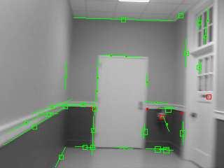
36 the edgelet is needed since the regularization parameter is added to summations over W E (j) values that depend on the length, in (3.22) and (3.23). The absolute value is needed in case π/2 < θ j < π, and the minimum value of 0.01 ensures that some regularization is always applied. The dependency on θ j causes the smoothing to be applied primarily along the edgelet rather than across the edgelet. For example, a vertical edgelet is pulled vertically by its neighbors, but its horizontal motion is determined primarily by local image data. Similarly, a horizontal edgelet is pulled horizontally by its neighbors, but its vertical motion is determined primarily by local image data. 27
37 Chapter 4 Results The unified point-edgelet feature tracking algorithm was implemented using the Blepo computer vision library and Microsoft Visual C++. The feature tracking algorithm was tested on the standard Middlebury optical flow datasets, and the average angular error and average endpoint error were measured. The feature tracking algorithm was also tested on man-made indoor environments like hallways and rooms and on a few natural sequences. These images were acquired using handheld camera or camera mounted on a robot with significant scale changes and large displacements. The unified feature tracking algorithm was tested on Intel dual-core 2.2GHz processor with 3GB RAM. The features were tracked well over multiple frames if there are sufficient features in the neighborhood to guide the motion computation. It was observed that isolated features, especially edglets, suffer from aperture problem. The features also get straddled when objects undergo occlusion/disocclusion. The feature tracking algorithm was tested for various algorithm parameters, and the results have been presented in this chapter. The point features are represented by red dots, the edgelets by blue/green lines. The yellow lines indicate the direction and magnitude of motion vectors. The square around the point feature or edgelet centre represents the scale at which the features are visble. The bigger the square, the lower the pyramidal levels at which the features are visible. 28
38 4.1 Comparison with ground truth and other methods The unified point-edgelet feature tracking algorithm was tested on five Middlebury optical flow datasets: Rubberwhale, Venus, Dimetrodon, Urban2, and Urban3. The algorithm was compared with the ground truth results given in the Middlebury optical flow site [2]. The algorithm was also compared with two similar feature tracking algorithms: standard Lucas-Kanade feature tracking method, and the joint tracking of features and edges. We also tested these algorithms on a synthetic image sequence of a hallway. Frame 2 of the hallway sequence was obtained by shifting Frame 1 to right by 7 pixels and down by 5 pixels. Rubberwhale, Venus and Dimetrodon sequences have sufficient texture and contain more point features than edgelets. Urban2, Urban3 and Hallway sequences represent man-made environments and contain more edgelets than point features. All the algorithms were tested with three pyramidal levels and twenty maximum iterations. The neighborhood features are chosen using a radius of 30 pixels. Each of the three feature tracking methods use a different feature detection method. Hence, we choose features such that each feature detection method accounts for few thousand pixels in the image. Therefore, the feature detection methods for standard Lucas-kanade and joint tracking method would detect few thousand point features. The feature detection for unified feature tracking would detect point features and edgelets such that the point features and edgels in the edgelets sum upto few thousand pixels. The images with the tracked features for all these tracking methods are shown in Figures 4.1a to 4.3f. For all the three feature tracking methods, we obtained two performance metrics: average endpoint error and average angular error. For the point features, we obtain endpoint error and angular error by comparing the ground truth results at that pixel location. However, for the edgelet features, we follow a different method. Since we use a parametric representation for the edgelets, the edgels can be obtained only by discretization. Edgelets may sometimes represent motion boundaries and some of the discrete edgels may lie on the other side of the motion boundaries. So we obtain endpoint error and angular error by comparing the ground truth results at that pixel location and its eight neighbors. The average endpoint error and average angular error for these sequences has been presented in Table 4.1. As can be observed from Table 4.1, the unified point-edgelet feature tracking method provides far better results as compared to the standard Lucas-Kanade method for all the image sequences. Moreover, the results are comparable to that of the joint feature tracking method for 29
39 Error Average endpoint error Average angular error Image Pixels LK JFT UPE LK JFT UPE Venus Rubberwhale Dimetrodon Urban Urban Hallway Table 4.1: Average Endpoint Error (in pixels) and Average Angular Error (in degrees) for five Middlebury image pairs. The tracking methods used were standard Lucas-Kanade(LK), joint feature tracking (JFT), and unified point-edgelet feature tracking (UPE). All three algorithms were tested with three pyramid levels and twenty maximum iterations. Dimetrodon, Venus and Rubberwhale sequences. For the Urban2, Urban3 and Hallway sequences, the unified feature tracking method performs better than the joint tracking method. This is due to the choice of neighboring features. In the joint tracking method, all features within a certain radius of a feature are chosen as neighboring features. The expected displacements of point features and edgelets is computed by fitting an affine motion model to these features. However, all these features are point features and do not capture the geometry of the image content completely. In the unified feature tracking method, we choose the neighboring features based on the geometry of the point features and edgelets. All point features and edgelets with endpoints within a certain radius of the point feature and all point features and edgelets with endpoints within a certain radius of the edgelet centre and endpoints are chosen as neighboring features. The expected displacements of point features and edgelets is computed by fitting an affine motion model as in the joint feature tracking method. Hence, it can be seen that more neighboring features are chosen based on feature geometry and hence the flow vector computation is more regularized. It can also be observed from Figures 4.2f, 4.3e, and 4.3f that a combination of edgelets and point features provide better representation of man-made environments. It can also be observed that these images contain multiple closely spaced edgelets which are tracked reliably using the unified feature tracking method. The edgelets which are typically attracted to nearby edges are guided by optical flow and regularization, and hence provide reliable flow estimates for these edgelets. It can also be observed from Figure 4.2f that the unified feature tracking algorithm provides a meaningful representation of poorly textured image sequences. The unified feature tracking algorithm currently does not handle errors caused due to motion discontinuities. Hence, edgelets which lie 30
 Dimetrodon:")
 Dimetrodon: Unified feature tracking")

40 (a) Dimetrodon: Standard Lucas-Kanade (b) Rubberwhale: Standard Lucas-Kanade (c) Dimetrodon: Joint Lucas-Kanade (d) Rubberwhale: Joint Lucas-Kanade (e) Dimetrodon: Unified feature tracking (f) Rubberwhale: Unified feature tracking Figure 4.1: Results of different feature tracking methods for Dimetrodon and Rubberwhale. 31
 Venus: Joint")
 Venus: Unified feature tracking (f)")

41 (a) Venus: Standard Lucas-Kanade (b) Hallway: Standard Lucas-Kanade (c) Venus: Joint Lucas-Kanade (d) Hallway: Joint Lucas-Kanade (e) Venus: Unified feature tracking (f) Hallway: Unified feature tracking Figure 4.2: Results of different feature tracking methods for Venus and Hallway. 32
 Urban3: Standard Lucas-Kanade")
")
 Urban3: Unified feature")

42 (a) Urban2: Standard Lucas-Kanade (b) Urban3: Standard Lucas-Kanade (c) Urban2: Joint Lucas-Kanade (d) Urban3: Joint Lucas-Kanade (e) Urban2: Unified feature tracking (f) Urban3: Unified feature tracking Figure 4.3: Results of different feature tracking methods for Urban2 and Urban3. 33
43 on motion boundaries are influenced erroneously by their neighboring features. This can be observed from Figures 4.1f and 4.3e where the edgelets stray away due to motion discontuinuities and occlusion/disocclusion. 4.2 Dense feature representation The unified feature tracking method tracks point features and edgelets using regularization. Since this method obtains optical flow information for all pixels with at least unidirectional texture, it produces a dense optical flow field when compared to the standard Lucas-Kanade method. The joint tracking method and unified feature tracking method can be used to compute dense optical flow fields when the number of point features and edgelets are increased. We performed several tests on Middlebury optical flow datasets to evaluate the performance of the unified feature tracking method for dense optical flow computation. We measured the error metrics, average endpoint error and average angular error, for standard Lucas-Kanade method, joint tracking method and unified feature tracking method by increasing the number of features. For the standard Lucas-Kanade method and joint feature tracking method, the first N good point features were chosen, where N is the number of pixels to be represented using features. For the unified feature tracking method, the edgelets were chosen such that the sum of edgels would account for 0.8*N and the point features would account for 0.2*N. For dense optical flow computation, we take into consideration all the edgels in an edgelet. It was assumed that all edgels in an edgelet will undergo same motion and hence have same optical flow information. The edgels that constitute an edgelet were obtained using edgelet parameters and Bresenham line algorithm. The point features and edgels were compared with the ground truth results and the error metrics were measured for the three feature tracking methods. A plot of the average endpoint/angular error with respect to the number of pixels with valid optical flow information was obtained. Figures 4.5a to 4.5d show the performance of the three feature tracking methods when the optical flow field becomes dense. Venus, Rubberwhale and Dimetrodon image sequences have sufficient texture and hence point feature tracking algorithms like standard Lucas-Kanade and joint feature tracking method perform well when the optical flow field grows denser. It can be observed from Figures 4.5a and 4.5c that the average endpoint error and angular error are comparable for all three methods even 34
44 Figure 4.4: The yellow lines denote the motion vectors. The box and shell at the bottom right move to the right while the textured cloth behind them moves to the left. Similarly the objects in the lower portion move to the left while the blanket behind them moves to the right. Notice that edgelets of these objects within the green boxes are moving in the wrong direction since they lie on motion boundaries. This is due to the influence of the neighboring features which move in the opposite direction. when the number of pixels with valid optical flow information increases. The angular error of unified feature tracking method for the Rubberwhale sequence is greater when compared to the other two methods. This is due to the fact that some of the edgelets which lie on motion boundaries are influenced by the erroneous motion of their neighboring features as seen in Figure 4.4. The features shown within the green boxes are moving in the wrong direction since they lie on motion boundaries. Hence, all the edgels that constitute these edgelets are steered in the wrong direction thereby causing high angular error. Urban2, Urban3 and Hallway sequences represent man-made environments and can be meaningfully represented using point features and edgelets. It can be observed from Figures 4.5b and 4.5d that the standard Lucas-Kanade method performs poorly on these sequences. The joint tracking method and unified feature tracking method perform comparably on these sequences. In the untextured Hallway sequence, the unified feature tracking algorithm performs better than the joint tracking method. It was also observed from these images that the unified feature tracking method provides the better results compared to the other feature tracking methods when motion discontinuities are absent as in Urban3 or Hallway sequence. The dense feature representation of the three feature tracking methods for the Rubberwhale sequence has been shown in Figures 4.6a to 4.6l. Each figure shows the features representing 1000, 3000, 5000 and 7000 pixels in the image. It can be inferred from these images that the unified feature tracking method provides a meaningful representation of image content as compared to the other 35
45 5 Venus 5 Rubberwhale 5 Dimetrodon Average endpoint error Average endpoint error Average endpoint error Average endpoint error No. of pixels Urban No. of pixels No. of pixels (a) Average endpoint error: Hidden texture Average endpoint error Urban No. of pixels Average endpoint error (b) Average endpoint error: Synthetic sequences No. of pixels Hallway No. of pixels 20 Venus 20 Rubberwhale 20 Dimetrodon Average angular error Average angular error Average angular error No. of pixels No. of pixels (c) Average angular error: Hidden texture No. of pixels 20 Urban2 20 Urban3 20 Hallway Average angular error Average angular error Average angular error No. of pixels No. of pixels (d) Average angular error: Synthetic sequences No. of pixels 36 Figure 4.5: Average endpoint and angular error for dense optical flow.
 5000 pixels: joint tracking (i) 5000 pixels: unified tracking (j) 7000 pixels: standard LK (k) 7000 pixels: joint tracking (l) 7000 pixels: unified tracking Figure 4.")
46 (a) 1000 pixels: standard LK (b) 1000 pixels: joint tracking (c) 1000 pixels: unified tracking (d) 3000 pixels: standard LK (e) 3000 pixels: joint tracking (f) 3000 pixels: unified tracking (g) 5000 pixels: standard LK (h) 5000 pixels: joint tracking (i) 5000 pixels: unified tracking (j) 7000 pixels: standard LK (k) 7000 pixels: joint tracking (l) 7000 pixels: unified tracking Figure 4.6: Notice that the unified feature tracking method provides a meaningful representation of the scene as compared to the other two methods for dense feature representation. 37
47 10 x 104 Venus 10 x 104 Rubberwhale 10 x 104 Dimetrodon Computation time (ms) Computation time (ms) Computation time (ms) No. of pixels No. of pixels (a) Computation time: Hidden texture No. of pixels 10 x 104 Urban2 10 x 104 Urban3 10 x 104 Hallway Computation time (ms) Computation time (ms) Computation time (ms) No. of pixels No. of pixels (b) Computation time: Synthetic sequences No. of pixels Figure 4.7: Computation time for different feature tracking methods. feature tracking methods. 4.3 Computation time The computation time of the standard Lucas-Kanade method, joint tracking method and unified feature tracking method was obtained for features representing different number of pixels. Features represent only point features for Lucas-Kanade method and joint tracking method. Both point features and edgelets are taken into account for unified feature tracking method. Figures 4.7a and 4.7b show the computation time for all the three feature tracking methods. It can be observed from Figures 4.7a and 4.7b that the Lucas-Kanade method takes only 100ms on an average even for a large number of features. However, the joint tracking method and 38
48 unified feature tracking method take atleast few hundreds of milliseconds and the computation time increases to few seconds as the number of features increase. This is due to the fact that both these methods rely on the motion vector computation of the neighboring features whereas the Lucas- Kanade method tracks features independently. It should also be noted that even though the unified feature tracking method tracks both point features and edgelets, its computation time is much lesser than that of the joint tracking method. This is due to the efficient feature representation in the unified feature tracking method. In the unified feature tracking method, all the edgels in a edgelet are tracked as a single feature. In the joint tracking method, each edgel would be tracked as a distinct point feature. Hence the unified feature tracking method, besides providing meaningful description of an image, can also be used for nearly real-time tracking. 4.4 Indoor image sequences Hallway sequence The unified feature tracking algorithm was tested using an image sequence of hallway taken using a handheld camera. The image sequence consisted of 300 frames. These images represent typical indoor image sequences with very less texture and relatively more edgelets. The feature tracking results for few frames have been shown in Figures 4.8a to 4.8o. This image sequence has various scale changes and large motion between successive frames. Hence, we use up to five pyramidal levels to handle large motion and maximum of 20 iterations. Since this image sequence has very few features, we choose any feature within a radius of 70 pixels as a neighboring feature. This ensures that there are sufficient features to provide flow vector regularization. Utilization of feature scale in this method has shown very reliable results. The scale of the tracked features was also updated in every frame. ItcanbeobservedfromFigures4.8cand4.8dandFigures4.8jand4.8kthatthesesubsequent frames show large displacment. However, our feature tracking method has been able to track features on these frames reliably. It can also be observed that we use a translational model for our feature tracking method and hence only the change in displacement of the edgelets is computed. Any change in orientation or length of the edgelets is not computed. Hence, when image frames have large viewpoint changes over a few frames, the edgelets tracked using this method will not align exactly with the image edges. 39
")
 Frame")

")
 Frame")

")
 Frame")

")
 Frame")

49 (a) Frame 50 (b) Frame 60 (c) Frame 74 (d) Frame 75 (e) Frame 90 (f) Frame 125 (g) Frame 150 (h) Frame 175 (i) Frame 200 (j) Frame 203 (k) Frame 204 (l) Frame 225 (m) Frame 250 (n) Frame 275 (o) Frame 305 Figure 4.8: Unified point-edgelet feature tracking on Hallway sequence. 40
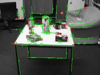
50 4.4.2 BoBoT sequence - C The unified feature tracking algorithm was tested using sequence C of Bonn Benchmark on Tracking (BoBoT). This sequence consists of 404 frames of a room obtained using a moving camera. This sequence represents another man-made environment with relatively more edgelets and texture due to presence of multiple objects. This sequence has large direction and scale changes and our feature tracking method has provided reliable results on this sequence. In order to handle large direction changes, we use up to four pyramidal levels and maximum of 20 iterations. Since this sequence has reasonably more point features and edgelets, any feature within a radius of 30 pixels is chosen as a neighboring feature. The feature tracking results have been shown in Figures 4.9a to 4.9o. 4.5 Effect of scale in tracking As described in Sections and , the scale at which the point features and edgelets can be detected is determined. The features are tracked only from the pyramidal level at which they can be detected. At lower pyramidal levels at which they cannot be detected, they follow the motion of the neighboring features. This ensures that the features do not give erroneous motion vectors at lower pyramidal levels at which they cannot be detected. This proves really very effective when there is large displacement between frames and multiple pyramidal levels are used. Figures 4.10a and 4.10b shows two images from the hallway sequence where the point features have been tracked without taking into account the scale at which these features can be detected. Figures 4.10c and 4.10d shows the same images where the features have been tracked giving respect to the scale at which they can be detected. The number of pyramidal levels, iterations and other parameters used in both the cases were the same. It can be observed from these images that some edgelets which represent the door frame stray away when tracked at all pyramidal levels. This is due to the fact that these edges have weak gradients and hence vanish at lower pyramidal levels. Hence, the motion vectors computed at lower pyramidal levels are erroneous and serve as wrong intialization vectors for upper pyramidal levels. When the features are tracked from the pyramidal levels at which they can be detected, they provide more reliable flow vectors. Figures 4.10c and 4.10d show that these edgelets which represent the door frame are visible only at the uppermost pyramidal level. Hence, these edgelets follow the neighboring features motion vectors at the lower 41
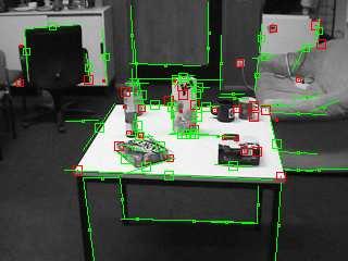
")
 Frame")

")
 Frame")

")
 Frame")

")
 Frame")


51 (a) Frame 2 (b) Frame 34 (c) Frame 55 (d) Frame 75 (e) Frame 100 (f) Frame 150 (g) Frame 172 (h) Frame 195 (i) Frame 227 (j) Frame 242 (k) Frame 275 (l) Frame 300 (m) Frame 350 (n) Frame 396 (o) Frame 404 Figure 4.9: Unified point-edgelet feature tracking on BoBoT sequence C. 42
 Frame 74 - Features")

 better than")
52 (a) Frame 74 - Features detected with no scale information (b) Frame 75 - Features tracked at all pyramidal levels (c) Frame 74 - Features detected in scale space (d) Frame 75 - Features tracked in scale space Figure 4.10: Note that the features tracked in scale space are able to handle features due to weak gradients (edgelets on the door frame) better than their counterpart which tracks all features at all pyramidal levels. 43
Feature Tracking and Optical Flow
 Feature Tracking and Optical Flow Prof. D. Stricker Doz. G. Bleser Many slides adapted from James Hays, Derek Hoeim, Lana Lazebnik, Silvio Saverse, who 1 in turn adapted slides from Steve Seitz, Rick Szeliski,
Motion Estimation. There are three main types (or applications) of motion estimation:
 of motion estimation:") Members: D91922016 朱威達 R93922010 林聖凱 R93922044 謝俊瑋 Motion Estimation There are three main types (or applications) of motion estimation: Parametric motion (image alignment) The main idea of parametric motion
Members: D91922016 朱威達 R93922010 林聖凱 R93922044 謝俊瑋 Motion Estimation There are three main types (or applications) of motion estimation: Parametric motion (image alignment) The main idea of parametric motion
Feature Tracking and Optical Flow
 Feature Tracking and Optical Flow Prof. D. Stricker Doz. G. Bleser Many slides adapted from James Hays, Derek Hoeim, Lana Lazebnik, Silvio Saverse, who in turn adapted slides from Steve Seitz, Rick Szeliski,
CS 4495 Computer Vision Motion and Optic Flow
 CS 4495 Computer Vision Aaron Bobick School of Interactive Computing Administrivia PS4 is out, due Sunday Oct 27 th. All relevant lectures posted Details about Problem Set: You may *not* use built in Harris
COMPUTER VISION > OPTICAL FLOW UTRECHT UNIVERSITY RONALD POPPE
 COMPUTER VISION 2017-2018 > OPTICAL FLOW UTRECHT UNIVERSITY RONALD POPPE OUTLINE Optical flow Lucas-Kanade Horn-Schunck Applications of optical flow Optical flow tracking Histograms of oriented flow Assignment
Peripheral drift illusion
 Peripheral drift illusion Does it work on other animals? Computer Vision Motion and Optical Flow Many slides adapted from J. Hays, S. Seitz, R. Szeliski, M. Pollefeys, K. Grauman and others Video A video
SIFT: SCALE INVARIANT FEATURE TRANSFORM SURF: SPEEDED UP ROBUST FEATURES BASHAR ALSADIK EOS DEPT. TOPMAP M13 3D GEOINFORMATION FROM IMAGES 2014
 SIFT: SCALE INVARIANT FEATURE TRANSFORM SURF: SPEEDED UP ROBUST FEATURES BASHAR ALSADIK EOS DEPT. TOPMAP M13 3D GEOINFORMATION FROM IMAGES 2014 SIFT SIFT: Scale Invariant Feature Transform; transform image
Motion. 1 Introduction. 2 Optical Flow. Sohaib A Khan. 2.1 Brightness Constancy Equation
 Motion Sohaib A Khan 1 Introduction So far, we have dealing with single images of a static scene taken by a fixed camera. Here we will deal with sequence of images taken at different time intervals. Motion
Using temporal seeding to constrain the disparity search range in stereo matching
 Using temporal seeding to constrain the disparity search range in stereo matching Thulani Ndhlovu Mobile Intelligent Autonomous Systems CSIR South Africa Email: tndhlovu@csir.co.za Fred Nicolls Department
Augmented Reality VU. Computer Vision 3D Registration (2) Prof. Vincent Lepetit
 Prof. Vincent Lepetit") Augmented Reality VU Computer Vision 3D Registration (2) Prof. Vincent Lepetit Feature Point-Based 3D Tracking Feature Points for 3D Tracking Much less ambiguous than edges; Point-to-point reprojection
Augmented Reality VU Computer Vision 3D Registration (2) Prof. Vincent Lepetit Feature Point-Based 3D Tracking Feature Points for 3D Tracking Much less ambiguous than edges; Point-to-point reprojection
Segmentation and Tracking of Partial Planar Templates
 Segmentation and Tracking of Partial Planar Templates Abdelsalam Masoud William Hoff Colorado School of Mines Colorado School of Mines Golden, CO 800 Golden, CO 800 amasoud@mines.edu whoff@mines.edu Abstract
CS 565 Computer Vision. Nazar Khan PUCIT Lectures 15 and 16: Optic Flow
 CS 565 Computer Vision Nazar Khan PUCIT Lectures 15 and 16: Optic Flow Introduction Basic Problem given: image sequence f(x, y, z), where (x, y) specifies the location and z denotes time wanted: displacement
Computer Vision Lecture 20
 Computer Perceptual Vision and Sensory WS 16/76 Augmented Computing Many slides adapted from K. Grauman, S. Seitz, R. Szeliski, M. Pollefeys, S. Lazebnik Computer Vision Lecture 20 Motion and Optical Flow
Visual Tracking (1) Feature Point Tracking and Block Matching
 Feature Point Tracking and Block Matching") Intelligent Control Systems Visual Tracking (1) Feature Point Tracking and Block Matching Shingo Kagami Graduate School of Information Sciences, Tohoku University swk(at)ic.is.tohoku.ac.jp http://www.ic.is.tohoku.ac.jp/ja/swk/
Intelligent Control Systems Visual Tracking (1) Feature Point Tracking and Block Matching Shingo Kagami Graduate School of Information Sciences, Tohoku University swk(at)ic.is.tohoku.ac.jp http://www.ic.is.tohoku.ac.jp/ja/swk/
Image processing and features
 Image processing and features Gabriele Bleser gabriele.bleser@dfki.de Thanks to Harald Wuest, Folker Wientapper and Marc Pollefeys Introduction Previous lectures: geometry Pose estimation Epipolar geometry
Visual Tracking. Image Processing Laboratory Dipartimento di Matematica e Informatica Università degli studi di Catania.
 Image Processing Laboratory Dipartimento di Matematica e Informatica Università degli studi di Catania 1 What is visual tracking? estimation of the target location over time 2 applications Six main areas:
Computer Vision Lecture 20
 Computer Perceptual Vision and Sensory WS 16/17 Augmented Computing Computer Perceptual Vision and Sensory WS 16/17 Augmented Computing Computer Perceptual Vision and Sensory WS 16/17 Augmented Computing
Multi-stable Perception. Necker Cube
 Multi-stable Perception Necker Cube Spinning dancer illusion, Nobuyuki Kayahara Multiple view geometry Stereo vision Epipolar geometry Lowe Hartley and Zisserman Depth map extraction Essential matrix
Dense Image-based Motion Estimation Algorithms & Optical Flow
 Dense mage-based Motion Estimation Algorithms & Optical Flow Video A video is a sequence of frames captured at different times The video data is a function of v time (t) v space (x,y) ntroduction to motion
Optic Flow and Basics Towards Horn-Schunck 1
 Optic Flow and Basics Towards Horn-Schunck 1 Lecture 7 See Section 4.1 and Beginning of 4.2 in Reinhard Klette: Concise Computer Vision Springer-Verlag, London, 2014 1 See last slide for copyright information.
Fundamental matrix. Let p be a point in left image, p in right image. Epipolar relation. Epipolar mapping described by a 3x3 matrix F
 Fundamental matrix Let p be a point in left image, p in right image l l Epipolar relation p maps to epipolar line l p maps to epipolar line l p p Epipolar mapping described by a 3x3 matrix F Fundamental
CS-465 Computer Vision
 CS-465 Computer Vision Nazar Khan PUCIT 9. Optic Flow Optic Flow Nazar Khan Computer Vision 2 / 25 Optic Flow Nazar Khan Computer Vision 3 / 25 Optic Flow Where does pixel (x, y) in frame z move to in
Visual Tracking (1) Tracking of Feature Points and Planar Rigid Objects
 Tracking of Feature Points and Planar Rigid Objects") Intelligent Control Systems Visual Tracking (1) Tracking of Feature Points and Planar Rigid Objects Shingo Kagami Graduate School of Information Sciences, Tohoku University swk(at)ic.is.tohoku.ac.jp http://www.ic.is.tohoku.ac.jp/ja/swk/
Intelligent Control Systems Visual Tracking (1) Tracking of Feature Points and Planar Rigid Objects Shingo Kagami Graduate School of Information Sciences, Tohoku University swk(at)ic.is.tohoku.ac.jp http://www.ic.is.tohoku.ac.jp/ja/swk/
Capturing, Modeling, Rendering 3D Structures
 Computer Vision Approach Capturing, Modeling, Rendering 3D Structures Calculate pixel correspondences and extract geometry Not robust Difficult to acquire illumination effects, e.g. specular highlights
Optical flow and tracking
 EECS 442 Computer vision Optical flow and tracking Intro Optical flow and feature tracking Lucas-Kanade algorithm Motion segmentation Segments of this lectures are courtesy of Profs S. Lazebnik S. Seitz,
Visual Tracking. Antonino Furnari. Image Processing Lab Dipartimento di Matematica e Informatica Università degli Studi di Catania
 Visual Tracking Antonino Furnari Image Processing Lab Dipartimento di Matematica e Informatica Università degli Studi di Catania furnari@dmi.unict.it 11 giugno 2015 What is visual tracking? estimation
Chapter 9 Object Tracking an Overview
 Chapter 9 Object Tracking an Overview The output of the background subtraction algorithm, described in the previous chapter, is a classification (segmentation) of pixels into foreground pixels (those belonging
Lecture 16: Computer Vision
 CS4442/9542b: Artificial Intelligence II Prof. Olga Veksler Lecture 16: Computer Vision Motion Slides are from Steve Seitz (UW), David Jacobs (UMD) Outline Motion Estimation Motion Field Optical Flow Field
Motion Estimation (II) Ce Liu Microsoft Research New England
 Ce Liu Microsoft Research New England") Motion Estimation (II) Ce Liu celiu@microsoft.com Microsoft Research New England Last time Motion perception Motion representation Parametric motion: Lucas-Kanade T I x du dv = I x I T x I y I x T I y
Motion Estimation (II) Ce Liu celiu@microsoft.com Microsoft Research New England Last time Motion perception Motion representation Parametric motion: Lucas-Kanade T I x du dv = I x I T x I y I x T I y
Motion and Optical Flow. Slides from Ce Liu, Steve Seitz, Larry Zitnick, Ali Farhadi
 Motion and Optical Flow Slides from Ce Liu, Steve Seitz, Larry Zitnick, Ali Farhadi We live in a moving world Perceiving, understanding and predicting motion is an important part of our daily lives Motion
Leow Wee Kheng CS4243 Computer Vision and Pattern Recognition. Motion Tracking. CS4243 Motion Tracking 1
 Leow Wee Kheng CS4243 Computer Vision and Pattern Recognition Motion Tracking CS4243 Motion Tracking 1 Changes are everywhere! CS4243 Motion Tracking 2 Illumination change CS4243 Motion Tracking 3 Shape
Image features. Image Features
 Image features Image features, such as edges and interest points, provide rich information on the image content. They correspond to local regions in the image and are fundamental in many applications in
Motion and Tracking. Andrea Torsello DAIS Università Ca Foscari via Torino 155, Mestre (VE)
") Motion and Tracking Andrea Torsello DAIS Università Ca Foscari via Torino 155, 30172 Mestre (VE) Motion Segmentation Segment the video into multiple coherently moving objects Motion and Perceptual Organization
Motion and Tracking Andrea Torsello DAIS Università Ca Foscari via Torino 155, 30172 Mestre (VE) Motion Segmentation Segment the video into multiple coherently moving objects Motion and Perceptual Organization
Comparison between Motion Analysis and Stereo
 MOTION ESTIMATION The slides are from several sources through James Hays (Brown); Silvio Savarese (U. of Michigan); Octavia Camps (Northeastern); including their own slides. Comparison between Motion Analysis
Colour Segmentation-based Computation of Dense Optical Flow with Application to Video Object Segmentation
 ÖGAI Journal 24/1 11 Colour Segmentation-based Computation of Dense Optical Flow with Application to Video Object Segmentation Michael Bleyer, Margrit Gelautz, Christoph Rhemann Vienna University of Technology
Other Linear Filters CS 211A
 Other Linear Filters CS 211A Slides from Cornelia Fermüller and Marc Pollefeys Edge detection Convert a 2D image into a set of curves Extracts salient features of the scene More compact than pixels Origin
CS664 Lecture #18: Motion
 CS664 Lecture #18: Motion Announcements Most paper choices were fine Please be sure to email me for approval, if you haven t already This is intended to help you, especially with the final project Use
Towards the completion of assignment 1
 Towards the completion of assignment 1 What to do for calibration What to do for point matching What to do for tracking What to do for GUI COMPSCI 773 Feature Point Detection Why study feature point detection?
Face Tracking : An implementation of the Kanade-Lucas-Tomasi Tracking algorithm
 Face Tracking : An implementation of the Kanade-Lucas-Tomasi Tracking algorithm Dirk W. Wagener, Ben Herbst Department of Applied Mathematics, University of Stellenbosch, Private Bag X1, Matieland 762,
Final Exam Study Guide
 Final Exam Study Guide Exam Window: 28th April, 12:00am EST to 30th April, 11:59pm EST Description As indicated in class the goal of the exam is to encourage you to review the material from the course.
Matching. Compare region of image to region of image. Today, simplest kind of matching. Intensities similar.
 Matching Compare region of image to region of image. We talked about this for stereo. Important for motion. Epipolar constraint unknown. But motion small. Recognition Find object in image. Recognize object.
EE795: Computer Vision and Intelligent Systems
 EE795: Computer Vision and Intelligent Systems Spring 2012 TTh 17:30-18:45 FDH 204 Lecture 14 130307 http://www.ee.unlv.edu/~b1morris/ecg795/ 2 Outline Review Stereo Dense Motion Estimation Translational
School of Computing University of Utah
 School of Computing University of Utah Presentation Outline 1 2 3 4 Main paper to be discussed David G. Lowe, Distinctive Image Features from Scale-Invariant Keypoints, IJCV, 2004. How to find useful keypoints?
CS231A Section 6: Problem Set 3
 CS231A Section 6: Problem Set 3 Kevin Wong Review 6 -! 1 11/09/2012 Announcements PS3 Due 2:15pm Tuesday, Nov 13 Extra Office Hours: Friday 6 8pm Huang Common Area, Basement Level. Review 6 -! 2 Topics
Lecture 19: Motion. Effect of window size 11/20/2007. Sources of error in correspondences. Review Problem set 3. Tuesday, Nov 20
 Lecture 19: Motion Review Problem set 3 Dense stereo matching Sparse stereo matching Indexing scenes Tuesda, Nov 0 Effect of window size W = 3 W = 0 Want window large enough to have sufficient intensit
Feature Detection. Raul Queiroz Feitosa. 3/30/2017 Feature Detection 1
 Feature Detection Raul Queiroz Feitosa 3/30/2017 Feature Detection 1 Objetive This chapter discusses the correspondence problem and presents approaches to solve it. 3/30/2017 Feature Detection 2 Outline
SUMMARY: DISTINCTIVE IMAGE FEATURES FROM SCALE- INVARIANT KEYPOINTS
 SUMMARY: DISTINCTIVE IMAGE FEATURES FROM SCALE- INVARIANT KEYPOINTS Cognitive Robotics Original: David G. Lowe, 004 Summary: Coen van Leeuwen, s1460919 Abstract: This article presents a method to extract
Ninio, J. and Stevens, K. A. (2000) Variations on the Hermann grid: an extinction illusion. Perception, 29,
 Variations on the Hermann grid: an extinction illusion. Perception, 29,") Ninio, J. and Stevens, K. A. (2000) Variations on the Hermann grid: an extinction illusion. Perception, 29, 1209-1217. CS 4495 Computer Vision A. Bobick Sparse to Dense Correspodence Building Rome in
Ninio, J. and Stevens, K. A. (2000) Variations on the Hermann grid: an extinction illusion. Perception, 29, 1209-1217. CS 4495 Computer Vision A. Bobick Sparse to Dense Correspodence Building Rome in
Computer Vision I - Filtering and Feature detection
 Computer Vision I - Filtering and Feature detection Carsten Rother 30/10/2015 Computer Vision I: Basics of Image Processing Roadmap: Basics of Digital Image Processing Computer Vision I: Basics of Image
Lecture 16: Computer Vision
 CS442/542b: Artificial ntelligence Prof. Olga Veksler Lecture 16: Computer Vision Motion Slides are from Steve Seitz (UW), David Jacobs (UMD) Outline Motion Estimation Motion Field Optical Flow Field Methods
VC 11/12 T11 Optical Flow
 VC 11/12 T11 Optical Flow Mestrado em Ciência de Computadores Mestrado Integrado em Engenharia de Redes e Sistemas Informáticos Miguel Tavares Coimbra Outline Optical Flow Constraint Equation Aperture
Visual Tracking (1) Pixel-intensity-based methods
 Pixel-intensity-based methods") Intelligent Control Systems Visual Tracking (1) Pixel-intensity-based methods Shingo Kagami Graduate School of Information Sciences, Tohoku University swk(at)ic.is.tohoku.ac.jp http://www.ic.is.tohoku.ac.jp/ja/swk/
Intelligent Control Systems Visual Tracking (1) Pixel-intensity-based methods Shingo Kagami Graduate School of Information Sciences, Tohoku University swk(at)ic.is.tohoku.ac.jp http://www.ic.is.tohoku.ac.jp/ja/swk/
Computational Optical Imaging - Optique Numerique. -- Single and Multiple View Geometry, Stereo matching --
 Computational Optical Imaging - Optique Numerique -- Single and Multiple View Geometry, Stereo matching -- Autumn 2015 Ivo Ihrke with slides by Thorsten Thormaehlen Reminder: Feature Detection and Matching
Announcements. Edges. Last Lecture. Gradients: Numerical Derivatives f(x) Edge Detection, Lines. Intro Computer Vision. CSE 152 Lecture 10
 Edge Detection, Lines. Intro Computer Vision. CSE 152 Lecture 10") Announcements Assignment 2 due Tuesday, May 4. Edge Detection, Lines Midterm: Thursday, May 6. Introduction to Computer Vision CSE 152 Lecture 10 Edges Last Lecture 1. Object boundaries 2. Surface normal
Announcements Assignment 2 due Tuesday, May 4. Edge Detection, Lines Midterm: Thursday, May 6. Introduction to Computer Vision CSE 152 Lecture 10 Edges Last Lecture 1. Object boundaries 2. Surface normal
ELEC Dr Reji Mathew Electrical Engineering UNSW
 ELEC 4622 Dr Reji Mathew Electrical Engineering UNSW Review of Motion Modelling and Estimation Introduction to Motion Modelling & Estimation Forward Motion Backward Motion Block Motion Estimation Motion
Announcements. Computer Vision I. Motion Field Equation. Revisiting the small motion assumption. Visual Tracking. CSE252A Lecture 19.
 Visual Tracking CSE252A Lecture 19 Hw 4 assigned Announcements No class on Thursday 12/6 Extra class on Tuesday 12/4 at 6:30PM in WLH Room 2112 Motion Field Equation Measurements I x = I x, T: Components
Outline 7/2/201011/6/
 Outline Pattern recognition in computer vision Background on the development of SIFT SIFT algorithm and some of its variations Computational considerations (SURF) Potential improvement Summary 01 2 Pattern
EECS 556 Image Processing W 09
 EECS 556 Image Processing W 09 Motion estimation Global vs. Local Motion Block Motion Estimation Optical Flow Estimation (normal equation) Man slides of this lecture are courtes of prof Milanfar (UCSC)
Computer Vision for HCI. Topics of This Lecture
 Computer Vision for HCI Interest Points Topics of This Lecture Local Invariant Features Motivation Requirements, Invariances Keypoint Localization Features from Accelerated Segment Test (FAST) Harris Shi-Tomasi
Autonomous Navigation for Flying Robots
 Computer Vision Group Prof. Daniel Cremers Autonomous Navigation for Flying Robots Lecture 7.1: 2D Motion Estimation in Images Jürgen Sturm Technische Universität München 3D to 2D Perspective Projections
International Journal of Advance Engineering and Research Development
 Scientific Journal of Impact Factor (SJIF): 4.72 International Journal of Advance Engineering and Research Development Volume 4, Issue 11, November -2017 e-issn (O): 2348-4470 p-issn (P): 2348-6406 Comparative
Edge and corner detection
 Edge and corner detection Prof. Stricker Doz. G. Bleser Computer Vision: Object and People Tracking Goals Where is the information in an image? How is an object characterized? How can I find measurements
BSB663 Image Processing Pinar Duygulu. Slides are adapted from Selim Aksoy
 BSB663 Image Processing Pinar Duygulu Slides are adapted from Selim Aksoy Image matching Image matching is a fundamental aspect of many problems in computer vision. Object or scene recognition Solving
Corner Detection. GV12/3072 Image Processing.
 Corner Detection 1 Last Week 2 Outline Corners and point features Moravec operator Image structure tensor Harris corner detector Sub-pixel accuracy SUSAN FAST Example descriptor: SIFT 3 Point Features
Feature Detectors and Descriptors: Corners, Lines, etc.
 Feature Detectors and Descriptors: Corners, Lines, etc. Edges vs. Corners Edges = maxima in intensity gradient Edges vs. Corners Corners = lots of variation in direction of gradient in a small neighborhood
Range Imaging Through Triangulation. Range Imaging Through Triangulation. Range Imaging Through Triangulation. Range Imaging Through Triangulation
 Obviously, this is a very slow process and not suitable for dynamic scenes. To speed things up, we can use a laser that projects a vertical line of light onto the scene. This laser rotates around its vertical
Visual motion. Many slides adapted from S. Seitz, R. Szeliski, M. Pollefeys
 Visual motion Man slides adapted from S. Seitz, R. Szeliski, M. Pollefes Motion and perceptual organization Sometimes, motion is the onl cue Motion and perceptual organization Sometimes, motion is the
Computer Vision Lecture 20
 Computer Vision Lecture 2 Motion and Optical Flow Bastian Leibe RWTH Aachen http://www.vision.rwth-aachen.de leibe@vision.rwth-aachen.de 28.1.216 Man slides adapted from K. Grauman, S. Seitz, R. Szeliski,
convolution shift invariant linear system Fourier Transform Aliasing and sampling scale representation edge detection corner detection
 COS 429: COMPUTER VISON Linear Filters and Edge Detection convolution shift invariant linear system Fourier Transform Aliasing and sampling scale representation edge detection corner detection Reading:
Computer Vision II Lecture 4
 Computer Vision II Lecture 4 Color based Tracking 29.04.2014 Bastian Leibe RWTH Aachen http://www.vision.rwth-aachen.de leibe@vision.rwth-aachen.de Course Outline Single-Object Tracking Background modeling
Lecture 20: Tracking. Tuesday, Nov 27
 Lecture 20: Tracking Tuesday, Nov 27 Paper reviews Thorough summary in your own words Main contribution Strengths? Weaknesses? How convincing are the experiments? Suggestions to improve them? Extensions?
Edge detection. Convert a 2D image into a set of curves. Extracts salient features of the scene More compact than pixels
 Edge Detection Edge detection Convert a 2D image into a set of curves Extracts salient features of the scene More compact than pixels Origin of Edges surface normal discontinuity depth discontinuity surface
Comparison Between The Optical Flow Computational Techniques
 Comparison Between The Optical Flow Computational Techniques Sri Devi Thota #1, Kanaka Sunanda Vemulapalli* 2, Kartheek Chintalapati* 3, Phanindra Sai Srinivas Gudipudi* 4 # Associate Professor, Dept.
Computer Vision I - Basics of Image Processing Part 2
 Computer Vision I - Basics of Image Processing Part 2 Carsten Rother 07/11/2014 Computer Vision I: Basics of Image Processing Roadmap: Basics of Digital Image Processing Computer Vision I: Basics of Image
Topological Mapping. Discrete Bayes Filter
 Topological Mapping Discrete Bayes Filter Vision Based Localization Given a image(s) acquired by moving camera determine the robot s location and pose? Towards localization without odometry What can be
Horn-Schunck and Lucas Kanade 1
 Horn-Schunck and Lucas Kanade 1 Lecture 8 See Sections 4.2 and 4.3 in Reinhard Klette: Concise Computer Vision Springer-Verlag, London, 2014 1 See last slide for copyright information. 1 / 40 Where We
CS201: Computer Vision Introduction to Tracking
 CS201: Computer Vision Introduction to Tracking John Magee 18 November 2014 Slides courtesy of: Diane H. Theriault Question of the Day How can we represent and use motion in images? 1 What is Motion? Change
Finally: Motion and tracking. Motion 4/20/2011. CS 376 Lecture 24 Motion 1. Video. Uses of motion. Motion parallax. Motion field
 Finally: Motion and tracking Tracking objects, video analysis, low level motion Motion Wed, April 20 Kristen Grauman UT-Austin Many slides adapted from S. Seitz, R. Szeliski, M. Pollefeys, and S. Lazebnik
Motion Analysis. Motion analysis. Now we will talk about. Differential Motion Analysis. Motion analysis. Difference Pictures
 Now we will talk about Motion Analysis Motion analysis Motion analysis is dealing with three main groups of motionrelated problems: Motion detection Moving object detection and location. Derivation of
Edge and local feature detection - 2. Importance of edge detection in computer vision
 Edge and local feature detection Gradient based edge detection Edge detection by function fitting Second derivative edge detectors Edge linking and the construction of the chain graph Edge and local feature
Chapter 3 Image Registration. Chapter 3 Image Registration
 Chapter 3 Image Registration Distributed Algorithms for Introduction (1) Definition: Image Registration Input: 2 images of the same scene but taken from different perspectives Goal: Identify transformation
Computer Vision I. Announcements. Fourier Tansform. Efficient Implementation. Edge and Corner Detection. CSE252A Lecture 13.
 Announcements Edge and Corner Detection HW3 assigned CSE252A Lecture 13 Efficient Implementation Both, the Box filter and the Gaussian filter are separable: First convolve each row of input image I with
Feature Based Registration - Image Alignment
 Feature Based Registration - Image Alignment Image Registration Image registration is the process of estimating an optimal transformation between two or more images. Many slides from Alexei Efros http://graphics.cs.cmu.edu/courses/15-463/2007_fall/463.html
Learning and Inferring Depth from Monocular Images. Jiyan Pan April 1, 2009
 Learning and Inferring Depth from Monocular Images Jiyan Pan April 1, 2009 Traditional ways of inferring depth Binocular disparity Structure from motion Defocus Given a single monocular image, how to infer
LOCAL-GLOBAL OPTICAL FLOW FOR IMAGE REGISTRATION
 LOCAL-GLOBAL OPTICAL FLOW FOR IMAGE REGISTRATION Ammar Zayouna Richard Comley Daming Shi Middlesex University School of Engineering and Information Sciences Middlesex University, London NW4 4BT, UK A.Zayouna@mdx.ac.uk
Local Feature Detectors
 Local Feature Detectors Selim Aksoy Department of Computer Engineering Bilkent University saksoy@cs.bilkent.edu.tr Slides adapted from Cordelia Schmid and David Lowe, CVPR 2003 Tutorial, Matthew Brown,
Using Geometric Blur for Point Correspondence
 1 Using Geometric Blur for Point Correspondence Nisarg Vyas Electrical and Computer Engineering Department, Carnegie Mellon University, Pittsburgh, PA Abstract In computer vision applications, point correspondence
EE795: Computer Vision and Intelligent Systems
 EE795: Computer Vision and Intelligent Systems Spring 2012 TTh 17:30-18:45 FDH 204 Lecture 10 130221 http://www.ee.unlv.edu/~b1morris/ecg795/ 2 Outline Review Canny Edge Detector Hough Transform Feature-Based
Augmented Reality, Advanced SLAM, Applications
 Augmented Reality, Advanced SLAM, Applications Prof. Didier Stricker & Dr. Alain Pagani alain.pagani@dfki.de Lecture 3D Computer Vision AR, SLAM, Applications 1 Introduction Previous lectures: Basics (camera,
3D Model Acquisition by Tracking 2D Wireframes
 3D Model Acquisition by Tracking 2D Wireframes M. Brown, T. Drummond and R. Cipolla {96mab twd20 cipolla}@eng.cam.ac.uk Department of Engineering University of Cambridge Cambridge CB2 1PZ, UK Abstract
Anno accademico 2006/2007. Davide Migliore
 Robotica Anno accademico 6/7 Davide Migliore migliore@elet.polimi.it Today What is a feature? Some useful information The world of features: Detectors Edges detection Corners/Points detection Descriptors?!?!?
Object Recognition with Invariant Features
 Object Recognition with Invariant Features Definition: Identify objects or scenes and determine their pose and model parameters Applications Industrial automation and inspection Mobile robots, toys, user
EN1610 Image Understanding Lab # 4: Corners, Interest Points, Hough Transform
 EN1610 Image Understanding Lab # 4: Corners, Interest Points, Hough Transform The goal of this fourth lab is to ˆ Learn how to detect corners, and use them in a tracking application ˆ Learn how to describe
CS 664 Segmentation. Daniel Huttenlocher
 CS 664 Segmentation Daniel Huttenlocher Grouping Perceptual Organization Structural relationships between tokens Parallelism, symmetry, alignment Similarity of token properties Often strong psychophysical
ROBUST LINE-BASED CALIBRATION OF LENS DISTORTION FROM A SINGLE VIEW
 ROBUST LINE-BASED CALIBRATION OF LENS DISTORTION FROM A SINGLE VIEW Thorsten Thormählen, Hellward Broszio, Ingolf Wassermann thormae@tnt.uni-hannover.de University of Hannover, Information Technology Laboratory,
AK Computer Vision Feature Point Detectors and Descriptors
 AK Computer Vision Feature Point Detectors and Descriptors 1 Feature Point Detectors and Descriptors: Motivation 2 Step 1: Detect local features should be invariant to scale and rotation, or perspective
The 2D/3D Differential Optical Flow
 The 2D/3D Differential Optical Flow Prof. John Barron Dept. of Computer Science University of Western Ontario London, Ontario, Canada, N6A 5B7 Email: barron@csd.uwo.ca Phone: 519-661-2111 x86896 Canadian
Biometrics Technology: Image Processing & Pattern Recognition (by Dr. Dickson Tong)
") Biometrics Technology: Image Processing & Pattern Recognition (by Dr. Dickson Tong) References: [1] http://homepages.inf.ed.ac.uk/rbf/hipr2/index.htm [2] http://www.cs.wisc.edu/~dyer/cs540/notes/vision.html
Biometrics Technology: Image Processing & Pattern Recognition (by Dr. Dickson Tong) References: [1] http://homepages.inf.ed.ac.uk/rbf/hipr2/index.htm [2] http://www.cs.wisc.edu/~dyer/cs540/notes/vision.html
C18 Computer vision. C18 Computer Vision. This time... Introduction. Outline.
 C18 Computer Vision. This time... 1. Introduction; imaging geometry; camera calibration. 2. Salient feature detection edges, line and corners. 3. Recovering 3D from two images I: epipolar geometry. C18
EE795: Computer Vision and Intelligent Systems
 EE795: Computer Vision and Intelligent Systems Spring 2012 TTh 17:30-18:45 FDH 204 Lecture 09 130219 http://www.ee.unlv.edu/~b1morris/ecg795/ 2 Outline Review Feature Descriptors Feature Matching Feature