ALGORITHMS AND INTERFACE FOR OCEAN ACOUSTIC RAY-TRACING (Developed in MATLAB)

Transcription

1 ALGORITHMS AND INTERFACE FOR OCEAN ACOUSTIC RAY-TRACING (Developed in MATLAB) Technical Report No. NIO/TR 09/005 T.V.Ramana Murty M.M.Malleswara Rao S.Surya Prakash P.Chandramouli K.S.R.Murthy Regional Centre, Visakhapatnam NATIONAL INSTITUTE OF OCEANOGRAPHY DONA PAULA, GOA , INDIA

2 CONTENTS Page No. ABSTRACT 1. INTRODUCTION 4. ELEMENTS OF OCEAN ACOUSTICS 6 3. RAY THEORY 8 4. COMPUTATION OF CANONICAL SOUND SPEED PROFILE METHODOLOGY 1 6. FLOW CHARTS SOFTWARE STRUCTURE 1 8. CASE STUDY 8 9. RESULTS ACKNOWLEDGEMENTS REFERENCES 3 1. APPENDIX-I CODING 33

3 ABSTRACT An integrated friendly-user interactive ocean application package has been developed for computation of eigenrays for a given source receiver configuration and subsurface and bottom environmental conditions utilizing the ray theory in MATLAB to study the Ocean Acoustic Propagation Characteristics (OAPS). This package facilitates automatic Graphical Visualization of acoustic ray parameters and generation of tabular forms of ray history for ray analysis. Results of numerical experiments conducted for Munk s canonical sound speed profile off Visakhapatnam waters are detailed as a case study. The simulated acoustic ray parameters of canonical ocean, off Visakhapatnam continental slope regions, reveals that the even very flat angle rays can scan entire water column with repeated reflections from both surface and bottom due to depth limited nature of sound channel and weak gradients of sound speed prevailing in the medium on either side of the sound channel axis. This nature of phenomenon usually occurs in the case of shallow-water channel. 3

4 INTRODUCTION: Acoustic waves which travel long distances in the ocean in the form of ducted propagation with less attenuation relative to other forms of energy, are used in a large number of applications in the ocean (Urick,R.J, 1983); for example, submarine signaling and detection, precise bathymetric measurements, sub-bottom profiling, fish finding etc. This is possible with the tracing of ray paths of sound pulses from a given source to a receiver in the ducted ocean of area of interest. Some of the common forms of ducts are: mixed layer sound channel, deep sound channel and shallow water sound channel. The surface sound channel (i.e., mixed layer sound channel) occurs when the upper layer exhibits isothermally leading to depth wise increase in the sound velocity, due to hydrostatic pressure. In this case the axis of the channel lies close to the sea surface. If an acoustic source is placed within this layer of constant velocity gradient, the acoustic energy gets trapped within this channel and propagation takes place along the rays that are in the form of arc of circles of radius of curvature R=C o /g where C o is surface sound velocity and g is velocity gradient. In the case of deep sound channel transmission experiments, sound sources and receivers are both placed preferably around the SOFAR (SOund Fixing And Ranging) channel axis (i.e., around the locus of points of minimum sound velocity). For example, in the tropical seas the sound velocity is between km below the ocean surface. This is due to the opposing effects of temperature, which dominates in the upper layers and causes a rapid decrease in sound speed with depth, and due to pressure, which increases eventually results in an increase of sound velocity. This configuration of the sound velocity profile in the vertical section of an ocean, which traps the sound rays around the sound axis, is called sound channel or SOFAR channel. Sound rays propagating along the SOFAR channel axis are refracted downward when propagating in the region of negative sound velocity gradient above the level of minimum sound velocity and upward when propagating in the region of positive gradient below it. The important feature of sound propagation along the SOFAR channel is that energy losses due to geometric spreading and scattering associated with the boundaries are 4

5 minimized and consequently large ranges of sound propagation are possible for the same source power (Officer C.B, 1958). In the present report, an automatic version of interface software (in MATLAB) to find out eigen rays (rays connecting between source and receiver) and related ray parameters are presented taking the example of Munk s canonical sound speed profile for continental slope waters off Visakhapatnam. This package works for nature of range independent as well as range-dependent environment with and without sloping bottom conditions. The systematic development of methodology starting from wave equation and its numerical computations with sample example detailed in the following sections. 5

6 ELEMENTS OF OCEAN ACOUSTICS Mathematical Formulation: Wave Equation: Acoustic wave propagation is an unsteady fluid flow problem related to mechanical vibration of ocean water in the range of tens of hertz to few hundred kilohertz. These vibrations are assumed to cause small departures from what is otherwise a static state in the fluid. As these vibrations are very fast and small, we ignore heat transfer between fluid elements. We also ignore viscosity since fluid motions are small. Now the equations governing this flow field are the continuity equation (Ramana Murty & Mahadevan, 1994) t. V 0 ( 1 ) and the momentum equation, V V. V P gk ( ) t where is the density of the fluid, V is the velocity of a fluid element with components (u,v,w), P is the pressure, k is a unit vector in the vertical (z) direction and g is the acceleration due to gravity. The flow variables associated with acoustic wave propagation problem, are treated as small departures from the undisturbed fluid state, and they are represented in the form = 0 + 1, V = V 0 + V 1 and P = P 0 + P 1. Here, the subscripts o denotes the undisturbed fluid state (i.e. the static state with V 0 = 0) and 1, the departures in field variables due to the presence of acoustic waves. Then, substituting these flow variables in Eqns. (1) and () and neglecting terms involving products of acoustic wave induced variables, we get the liberalized form of the governing equations as t and 1.( V1) 0 ( 3 ) 0 ( 0V 1) P1 ( 4 ) t eliminating V 1 between these equations, we get 1 t P 1 ( 5 ) 6

7 The frequency of acoustic oscillations is quite high and the associated pressure fluctuations in the fluid could be assumed as adiabatic. Then the equation of state is given by P 1 = C 1 and eqn. (5) can be written as (subscript is omitted for convenience). t P C P, ( 6 ) Where C is the sound speed through the propagating medium. The above equation, referred to as the wave equation, defines the pressure field associated with acoustic waves propagating in ocean waters. The solution to this equation (i.e. to the acoustic wave propagation problem in ocean waters) can be approached by acoustic ray theory applicable to high frequency waves or the normal mode theory. We will discuss here the ray theory, which has been successfully used in ocean acoustic tomography and other relevant sound propagation studies(ref:..). 7

8 RAY THEORY: Ray theory is widely used in underwater acoustics since it has many advantages. Some of them are 1) Rays are easily drawn ) Real boundary conditions are inserted easily, e.g. a sloping bottom 3) It is independent of source. This method is based on an equation called eikonel equation. This eikonel equation is obtained from the wave equation by assuming the solution in a particular form. We initially seek a periodic solution in time to the wave equation in the form P(x,y,z,t) = p(x,y,z) exp( -it ). This reduces the wave equation to the Helmholtz equation given by, p k p 0 ( 7 ) Where k = / C, is the wave number. The variation in sound speed in the ocean is very small and the solution to the Helmholtz equation can be assumed in the form p(x,y,z) = A(x,y,z) exp [i k 0 W(x,y,z)], ( 8 ) Where A is a slowly varying function of position, k 0 is a constant reference wave number and W is called the eikonel function. The functional form of this solution can be easily recognized to be the same as that of a plane wave solution in a homogeneous medium. i.e., P(x,y,z) = A exp{ i S(x,y,z,t) } ( 9 ) Where A is the constant amplitude of the wave and S(x,y,z,t) = k x X + k y Y + k z Z - t Is called the phase function. Here k x, k y, k z are the components of the wave number vector K of the plane wave. Note that, for a non-homogeneous medium, from eqn. (8), the phase function can be defined as S(x,y,z,t) = k 0 W(x,y,z) - t Substituting the solution, eqn. ( 8 ), in the Helmholtz equation, the real part gives W. W /( k 0 C ) A/( k 0 A) ( 10 ) The RHS of the above equation can be shown to be small when the variation of C is small over one wavelength of an acoustic wave. This condition is 8

9 satisfied in the case of high frequency sound propagation in ocean waters. Then we get W. W n ( 11 ) where the refractive index n = C 0 / C, is a function of position and C 0 = /k 0. The eqn. (11) is called the eikonel equation. Now at any time t, S(x,y,z,t) = constant, implies that the eikonel function is constant. Hence W = constant defines a surface of constant phase and W defines the normal to the surface of constant phase or the direction of ray propagation or ray path. In eq. (11), ray path and n is the magnitude of this vector. W is a vector in the direction of Let dr = (dx, dy, dz) be the displacement vector along the ray path and ds = dr. Then dr dx dy dz n n,, W ( 1 ) ds ds ds ds d dx d W dw Now n ds ds ds x x ds W dx W dy W dz = x x ds y ds z ds Hence we get = dx dy dz n n x ds ds ds x d ds dx n ds n d dy n, n and x ds ds y ( 13 a, b, c ) d dz n ds ds These equations state that the variation along the ray path of the product of the index of refraction and the direction cosine is equal to the space rate of variation of the index of refraction with respect to the appropriate coordinate. Eqns. (13) are the generalized form of Snell s law. Let us consider the sound propagation problem in two dimension in x-z plane (see Fig. A1). Then along the ray path n z 9

10 dx cos ds dz and sin ds (14 a,b ) Substituting eq. (14 a) in (13 a) and n = C 0 / C, we get along the x-direction d ds Similarly along the z-direction C 0 / C cos C 0 / C x C dc d cos CSin ( 15 ) x ds ds C dc d Sin CCos z ds ds Eliminating dc/ds from eqs. (15) and (16), we get d 1 C Sin ds C x Cos C z ( 16 ) ( 17 ) Now the eqs. (14) and (17) describe the ray paths and the numerical integration of these equations for a given sound speed distribution, provides the coordinates of the ray paths. Intensity computations The acoustic intensity at any point along the ray path is given by the expression (Krol H.R, 1979). x I (sin / xcos ).( / ) Intensity I (18) / z where I 0 reference intensity at the source; 0 eigen ray angle at the source with reference ti the horizontal; ray angle at the point of measurement with reference to the horizontal; X=distance from the source to the point of measurement; z vertical distance at the point of measurement between eigen ray and ray in its immediate vicinity; and 0 angle between eigen ray and ray in its immediate vicinity at the source. At the point where z 0, the above expression will not hold good (tends to infinity mathematically) and the previous value only gets substituted for computational continuity. Considering the phase shift for any given frequency the intensity has been computed following (Moler C B & Soloman L.P, 1970). 10

11 I i ftk I P e 0 where P I x 1/ Pj Pk f t j tk j k cos (19) k k /I 0 and t k are the relative pressures and arrival times of the eigen rays. These have wider applications in signal detection. COMPUTATION OF CANONICAL SOUND SPEED PROFILE : For simulation studies a parametric representation of the sound-speed profile is needed. In the present study, we construct a representative sound speed profile of waters of Visakhapatnam in an analytical form following Munk'(1974). The mathematical expression for generation of canonical sound speed profile has been detailed. The theory enables us to present the sound-speed profile at any geographical location with the help of a few parameters obtained from hydrographic data, apart from its implication in ray theory and normal mode theory. The Canonical expression for the sound velocity profile C(Z) (Munk,1974) expressed as function of a depth, stratification scale and perturbation coefficient as follows: 1 ( ZW B) exp( W ) 1) C ( Z) C1 B (0) where W Z Z1, (Z 1 is depth of sound channel axis) B a b (Stratification scale), 3 a (Perturbation coefficient b 1 r r a, b W 4 1, dw 3 W 5 r r dw, W 6 3 dw, 1 (a,b,c) 1 1 r f ( W ) W dw 1 (d) 11

12 1 r 3 f ( W ) W dw 1 (e) The above integrals can be evaluated using natural cubic spline interpolation technique for given sound speed profile, depth of sound channel axis, speed of sound at channel axis and upper and lower bounds of sound speed profile to get stratification scale and perturbation coefficient. METHODOLOGY Numerical ray tracing --- The solution of ray tracing with initial conditions specifying any given point (source coordinates and direction) on the ray is usually known as the initial-value problem. The numerical computations in the form of algorithm (Ramana Murty et.al, 1990) for Eqs 14(a,b) and 17 are : X 1 ij fi( X 1, X, X 3, X 4) 4 X X ds ( Z B Z A.() i i j 1 i j ' i ) j Z ' i Z i 3 4 j 1 ( Z i B j Z ' i ) A j C Z j i where i = 1,,3,4; Z 1=1; Z cos ; Z 3 sin ; Z 4 cos V z / V ; and with initial conditions of X 1 (0) 0 X ( 0) X 0( sourcex coordinate) X 3( 0) Z0( sourcey coordinate) X 4( 0) 0( horizontalangle) the coefficients of A j, B j and C j being: A 1/, B, C 1/ C 4 A 1 1/, B 1, C 1 1/ / 1 3 A 1/, B 1, C 1/ A 6, B 4 1, 1/ In the present study Runga-Kutta-Gill s method has been chosen to obtain the numerical solution. For the present analysis, step-size (ds) is chosen depending on the medium at the end point of the ray segment. In the 1

13 region of thermocline or halocline, ds is considered small compared to that within the layers further below and characterized by high gradients in sound speed. The changes in the range(dx), depth(dz) and the angle(d ) are computed. During integration, if the ray path does not pass through the nodal points which would define sound speed field for computing the gradients and the refractive index, they may be restricted to pass through arbitrary points in the plane. In such case, suitable interpolation function has to be defined to evaluate both sound speed and its partial derivatives for a given ds. A 3-point Lagrangian interpolation is used here to construct such a function along the vertical and in the neighborhood of the sound speed field taking points above and one point below and vice verse, prior to averaging. Knowing the information along ds and at arbitrary points, integration is carried out using the Runga-Kutta-Gill s technique. At the upper and lower boundaries, the ray gets reflected following equal angle law. Irregular bathymetric features and the curvature of the earth have not been considered here. The integration repeats until all rays within a given beam arrive at the receiver. If not, the algorithm takes on computation of the ray having the next assigned angle and follows the same procedure ( Shooting method ). The ray co-ordinates are kept in memory space allocated in a matrix form. The time of flight ( T i ) is determined following the recurrence formula 4 Y BjZ Y3 BjZ3 T T A ds () i i j 1 where i covers full range. Once the eigen rays are identified from the ray computation, the intensity calculations are made following the ray tube method. j 13

14 Generation canonical sound speed profile: The collected hydrographic data on temperature, salinity off waters of Visakhapatnam during March, 11-0, 1987 on ORV Sagarkanya has been used to generate canonical sound speed profile based on algorithm developed by Ramana Murty et.al, 1989 as a input profile for conducting numerical acoustic modeling. Initially the data was subjected to cubic spline (for continous data) and weighted parabolic (for discrete data) interpolation (Reininger and Ros 1968) to obtain observations at closely spaced depths (10m) intervals. From these data the sound speed has been computed following Chen Millerio(1977) to obtain the sound speed at the channel axis ( C 1), the depth of the channel axis ( Z 1 ) and upper and lower bounds of integration (, ) for the integrals appearing in Eqs.1(a-e) for computation of the stratification scale B and perturbation coefficient. Computed Canonical sound channel model parameters:- 50( m), 490( m), Z B ( km), ( m), C ( m / s) Using Canonical sound channel model parameters the following Munk s canonical sound speed profile is generated using Eq. 0 Sound speed profile (Here column 1 is Depth(m) and column is Sound speed(m/sec)) Before starting of the profile (-1 x) is been given which are detailed below: -1 is the flag which indicates starting of the profile. x indicates the range of the profile with reference to the previous profile File should contain two sets of profiles. (i) Range Independent In this case the profile should be repeated twice (ii) Range Dependent -- In this case the profiles are to be followed in range dependent nature. 14

15 Depth(m) Speed(m/sec) Depth(m) Speed(m/sec) Depth(m) Speed(m/sec) Depth(m) Speed(m/sec) Depth(m) Speed(m/sec)

16 Source and Receiver Depth at 1490m. 16

17 Flow Charts 17

18 START B Display Menu Select and Edit SSP I/P Data file Select and Edit BTH I/P file & Enable Ray file Button Select and Edit Ray I/P file & Enable Run Model Button User Selection == Run Model Button Y N Refresh the Program Enable Plot button B User Selection == Plots Button Y N Refresh the Program Display Graphs Enable Save & Print Buttons B STOP 18

19 Context Level DFDs Input Details User Ray Tracing Model Output Details 19

20 LOWER LEVEL DFD FOR RAY TRACING User I/P Filename with path (.ssp) I/P Filename with path (.bth) Ray Model Execution Generating O/P for plots O/P Plots I/P Filename with path (.ray) 0

21 Top Level DFDs Top Level DFD for Ray Tracing Hard Disk Input File name Data Output plots User Reading Input File (*) Ray Tracing Process Hard Disk Input Input Output File Show Input Process Input File Output Show Output Process (*) Files of (SSP,BTH AND RAY) have to be given simultaneously. 1

22 The following input files are used in the present developed software (Appendix-I) and sequential step wise operations are detailed in the next section. INPUT FILES Filename: munk.ssp Filename: test.bth Filename: ex1.ray SOFTWARE STRUCTURE A Main MATLAB script, Ray, is invoked from the MATLAB Command Window. This brings up the Main Graphical User Interface (GUI), which is populated by PUSH BUTTONS i.e., Ray File, SSP File, BTH File, RUN MODEL, PLOTS, REFRESH, Print Plots, SAVE PLOT and EXIT is shown in FIG 1. FIG 1.

23 Step wise Process On clicking on the PUSH BUTTON named SSP File allows the user to select the input for the list box as shown in FIG. FIG. Next selecting the Bathymetry profile by clicking on the PUSH BUTTON named BTH File as shown in FIG 3. This enables the PUSH BUTTON s named Ray File and RUN MODEL. FIG 3. Clicking on the PUSH BUTTON Ray File allows the list box as shown in FIG 4. on selecting the file from the list pops up the Ray file which consists of data regarding source, receiver, depth etc., 3

24 FIG 4. Now the system is ready for execution as the input files i.e., Sound Speed Profiles (.ssp), Bathymetry File (.bth) and Ray File (.ray) are given. Click on the PUSH BOTTON named RUN MODEL, after the execution of program the PUSH BOTTON s namely PLOTS, SAVE PLOT and Print Plots are enabled. On clicking on the plots displays the list box which is shown in FIG 5. which lists the four varieties of plots that has to be displayed namely Eigenrays, Bathmetry, Ztheta and Stick. FIG 5. 4

25 Selecting Eigenrays in the list box (FIG 5.) displays the plot in the form as shown in FIG 6. FIG 6. 5

26 Selecting Bathymetry in the list box (FIG 5.) displays the plot in the form as shown in FIG 7. FIG 7. 6

27 Selecting Ztheta in the list box (FIG 5.) displays the plot in the form as shown in FIG 8. FIG 8. 7

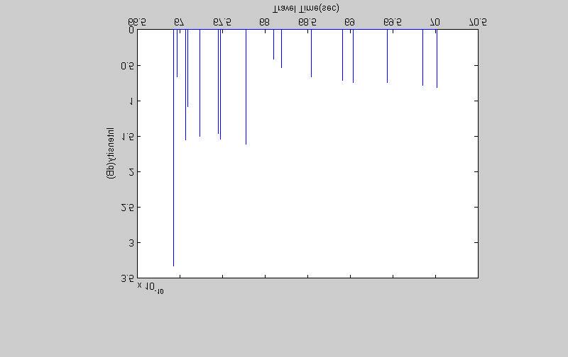
28 Selecting Stick in the list box (FIG 5.) displays the plot in the form as shown in FIG 9. FIG 9. Above plots can be saved by clicking on the PUSH BUTTON named SAVE PLOT, which pops a input box as shown in FIG 10 asking for the name by which the plot has to be stored. FIG 10. 8

29 CASE STUDY This interface is applied for Ocean Data. MUNK s canonical Sound Speed Profiles are taken into consideration. The output is as shown in FIG FIG 11. 9

30 FIG 1. 30

31 FIG

32 Results Following Munk s canonical theory, canonical parameters (i.e., B the stratification scale and the perturbation coefficient) in adiabatic ocean obtained using deduced SOFAR channel parameters (i.e., C 1 sound speed at the channel axis, Z 1 the depth of the channel axis) from the CTD data collected on board ORV Sagarkanya Cruise No.30 at N, E, in the Bay of Bengal to develop the stratified model for implementation in the numerical ray tracing to study the ocean acoustic parameters namely eigen rays, travel time, turning depths, transmission loss etc., for source-receiver configuration kept at channel axis. The simulated acoustic ray parameters of canonical ocean reveals that the even very flat angle rays can scan entire water column with repeated reflections from both surface and bottom due to depth limited nature of sound channel and weak gradients of sound speed prevailing in the medium on either side of the sound channel axis. This nature of phenomenon usually occurs in the case of shallow-water channel. Since the results are generated through simplest sound channel (exponential stratified model) above and beneath the sound axis would be more useful as aprior knowledge before conducting actual sound transmission experiment in the area of interest. Acknowledgements The authors are thankful to Dr.S.R.Shetye, Director, National Institute of oceanography, for his constant encouragement and keen interest in this study. 3

33 References 1. Urick,R.J, (1983) Principles of Underwater Sound, McGraw- Hill, Inc.. Officer C.B, (1958) Introduction To The Theory Of Sound Transmission, McGraw-Hill, Inc. USA. 3. Ramana MurtyT.V, Mahadevan.R (March 1994), Stochastic Inverse Method for Ocean Acoustic Tomography Studies A Simulation Experiment, IIT Technical Report No Krol H R, J Acoust Soc Am, 53(1973) Moler C B & Solomom L P, J Acoust Soc Am,48(1970) Munk W H(1974) Sound Channel in an exponentially stratified ocean with application to SOFAR J.Acoust.SOC.AM Ramana Murty T V, Somayajulu Y K & Sastry J S (1990) Computations of some acoustic ray parameters in the Bay of Bengal, IJMS,Vol. 19, pp Ramana Murty T V, Prasanna Kumar S, Somayajulu Y K, Sastry J S and Rui J P De Figueiredo. (October 1989) Canonical sound speed profile for the central Bay of Bengal. Earth Planet Sci., Vol 98, No: 3, July, pp Reiniger R F and Ros C K. (1968) A method of interpolation with application to oceanographic data; Deep Sea Res Chen C T and Millero F J. (1977) Speed of sound in sea water at higher pressure; J.Acoust.Soc,Am.55,

34 Appendix-I This invokes the GUI interface for Sound Propagation in Duct and Deep waters Created on September 10th NIO, RC, Visakhapatnam function varargout = ray(varargin) % Ref: WHOI Technical Report WHOI Ocean Acoustic Ray-Tracing % Software RAY, Bowlin,et.al., October, 199 % ray M-file for ray.fig % ray, by itself, creates a new ray or raises the existing % singleton*. % % H = ray returns the handle to a new ray or the handle to % the existing singleton*. % % ray('property','value',...) creates a new ray using the % given property value pairs. Unrecognized properties are passed via % varargin to ray_openingfcn. This calling syntax produces a % warning when there is an existing singleton*. % % ray('callback') and ray('callback',hobject,...) call the % local function named CALLBACK in ray.m with the given input % arguments. % % *See GUI Options on GUIDE's Tools menu. Choose "GUI allows only one % instance to run (singleton)". % % Edit the above text to modify the response to help ray % Last Modified by GUIDE v.5 01-Oct :3:37 % Begin initialization code - DO NOT EDIT gui_singleton = 1; gui_state = struct('gui_name', mfilename,... 'gui_singleton', gui_singleton,... 'gui_layoutfcn', [],... 'gui_callback', []); if nargin & isstr(varargin{1}) gui_state.gui_callback = strfunc(varargin{1}); end if nargout [varargout{1:nargout}] = gui_mainfcn(gui_state, varargin{:}); else gui_mainfcn(gui_state, varargin{:}); end 34

35 % End initialization code - DO NOT EDIT % --- Executes just before ray is made visible. function ray_openingfcn(hobject, eventdata, handles, varargin) % This function has no output args, see OutputFcn. % hobject handle to figure % eventdata reserved - to be defined in a future version of MATLAB % handles structure with handles and user data (see GUIDATA) % varargin unrecognized PropertyName/PropertyValue pairs from the % command line (see VARARGIN) % Choose default command line output for ray handles.output = hobject; handles.root = ''; handles.refresh= ''; set( [handles.ssp],'enable', 'on' ); set( [handles.bth], 'enable', 'on' ); set( [handles.print], 'enable', 'off' ); set( [handles.ray], 'enable', 'off' ); set( [handles.plots], 'enable', 'off' ); set( [handles.runmodel], 'enable', 'off' ); set( [handles.exit], 'enable', 'on' ); set( [handles.refresh], 'enable', 'on' ); set( [handles.save], 'enable', 'off' ); % Update handles structure guidata(hobject, handles); % UIWAIT makes ray wait for user response (see UIRESUME) % uiwait(handles.figure1); % --- Outputs from this function are returned to the command line. function varargout = ray_outputfcn(hobject, eventdata, handles) % varargout cell array for returning output args (see VARARGOUT); % hobject handle to figure % eventdata reserved - to be defined in a future version of MATLAB % handles structure with handles and user data (see GUIDATA) % Get default command line output from handles structure varargout{1} = handles.output; % --- Executes on button press in Ray. function Ray_Callback(hObject, eventdata, handles) % hobject handle to Ray (see GCBO) % eventdata reserved - to be defined in a future version of MATLAB % handles structure with handles and user data (see GUIDATA) 35

36 global FNAME d = dir('*.ray'); if isempty( d ) errordlg( 'Ray Files Not Found', 'Error' ); else filenames = {d.name}; [ s, v ] = listdlg( 'PromptString', 'Select a Input Data File :',... 'SelectionMode', 'single',... 'ListSize',[150,90],... 'Name','Ray File',... 'ListString', filenames ); handles.viewsourcefile = char( filenames( s ) ); handles.root = handles.viewsourcefile( 1:length( handles.viewsourcefile ) - 4 ); FNAME=handles.viewSourceFile if ( isempty( handles.viewsourcefile ) ) warndlg( 'No Input Ray File Has Been Selected', 'Warning' ); else h = questdlg('save files with(.ray) Extension','Warning','OK','OK') if (h=='ok') eval( [ '!write ' handles.viewsourcefile ] ); end end set( hobject, 'Value', 1.0 ); % show pushed end set( [handles.runmodel], 'enable', 'on' ); % Update handles structure guidata(hobject, handles); % --- Executes on button press in Ssp. function Ssp_Callback(hObject, eventdata, handles) % hobject handle to Ssp (see GCBO) % eventdata reserved - to be defined in a future version of MATLAB % handles structure with handles and user data (see GUIDATA) d = dir('*.ssp'); if isempty( d ) errordlg( 'Sound Speed Files Not Found', 'Error' ); else filenames = {d.name}; [ s, v ] = listdlg( 'PromptString', 'Select a Input Data File :',... 'SelectionMode', 'single',... 'ListSize',[150,90],... 'Name','Sound Speed File',... 'ListString', filenames ); handles.viewsourcefile = char( filenames( s ) ); handles.root = handles.viewsourcefile( 1:length( handles.viewsourcefile ) - 4 ); 36

37 if ( isempty( handles.viewsourcefile ) ) warndlg( 'No Input Sound Speed File Has Been Selected', 'Warning' ); else h = questdlg('save files with(.ssp) Extension','Warning','OK','OK') if (h=='ok') eval( [ '!write ' handles.viewsourcefile ] ); end end set( hobject, 'Value', 1.0 ); % show pushed end % Update handles structure guidata(hobject, handles); % --- Executes on button press in Bth. function Bth_Callback(hObject, eventdata, handles) % hobject handle to Bth (see GCBO) % eventdata reserved - to be defined in a future version of MATLAB % handles structure with handles and user data (see GUIDATA) d = dir('*.bth'); if isempty( d ) errordlg( 'Bathymetry Files Not Found', 'Error' ); else filenames = {d.name}; [ s, v ] = listdlg( 'PromptString', 'Select a Input Data File :',... 'SelectionMode', 'single',... 'ListSize',[150,90],... 'Name','Bathymetry File',... 'ListString', filenames ); handles.viewsourcefile = char( filenames( s ) ); handles.root = handles.viewsourcefile( 1:length( handles.viewsourcefile ) - 4 ); if ( isempty( handles.viewsourcefile ) ) warndlg( 'No Input Bathymetry File Has Been Selected', 'Warning' ); else h = questdlg('save files with(.bth) Extension','Warning','OK','OK') if (h=='ok') eval( [ '!write ' handles.viewsourcefile ] ); end end set( hobject, 'Value', 1.0 ); % show pushed end set( [handles.ray], 'enable', 'on' ); 37

38 set( [handles.ssp],'enable', 'off' ); set( [handles.bth], 'enable', 'off' ); % Update handles structure guidata(hobject, handles); % --- Executes on button press in Print. function Print_Callback(hObject, eventdata, handles) % hobject handle to Print (see GCBO) % eventdata reserved - to be defined in a future version of MATLAB % handles structure with handles and user data (see GUIDATA) print -depsc -tiff ms.eps print -dtiff -r00 ms.tiff % --- Executes on button press in EXIT. function EXIT_Callback(hObject, eventdata, handles) % hobject handle to EXIT (see GCBO) % eventdata reserved - to be defined in a future version of MATLAB % handles structure with handles and user data (see GUIDATA) closereq; % --- Executes on button press in runmodel. function runmodel_callback(hobject, eventdata, handles) % hobject handle to runmodel (see GCBO) % eventdata reserved - to be defined in a future version of MATLAB % handles structure with handles and user data (see GUIDATA) global FNAME dis=dos(['ray ' FNAME]) % Executes Ray.exe with the name as selected in the % list box when Push Botton Ray File is clicked. if (dis==0) eval(['!ray <' FNAME ' > out.txt']) %eval(['!ray <' FNAME ' > out.txt exit &']) eval('!exit&') msgbox('model Executed Successfully','Success','help','modal'); set( [handles.ray], 'enable', 'off' ); set( [handles.plots], 'enable', 'on' ); set( [handles.runmodel], 'enable', 'off' ); else msgbox('check input files','error','error','modal'); set( [handles.runmodel], 'enable', 'off' ); end % --- Executes on button press in Plots. function Plots_Callback(hObject, eventdata, handles) % hobject handle to Plots (see GCBO) % eventdata reserved - to be defined in a future version of MATLAB % handles structure with handles and user data (see GUIDATA) eval('load ex1.mat') str={'eigenrays','bathmetry','ztheta','stick'}; [ s, v ] = listdlg('promptstring','select a file:',... 38

39 'SelectionMode','single',... 'ListSize',[90,90],... 'Name','Select a Plot',... 'ListString',str) if(v==0) msgbox('no Plot is selected','warning','warn','modal'); end switch(s) case{1} eval('plotpath(eigenrays)'); % Plots Eigenrays set( [handles.save], 'enable', 'on' ); set( [handles.print], 'enable', 'on' ); case{} eval('plotbath(btab)'); % Plots Bathymetry set( [handles.save], 'enable', 'on' ); set( [handles.print], 'enable', 'on' ); case{3} eval('plotzthe(eigenrays)'); % Plots Ztheta set( [handles.save], 'enable', 'on' ); set( [handles.print], 'enable', 'on' ); case{4} eval('stickem'); % Plots Stick set( [handles.save], 'enable', 'on' ); set( [handles.print], 'enable', 'on' ); end %eval('clear all') % --- Executes on button press in Refresh. function Refresh_Callback(hObject, eventdata, handles) % hobject handle to Refresh (see GCBO) % eventdata reserved - to be defined in a future version of MATLAB % handles structure with handles and user data (see GUIDATA) closereq ray % --- Executes when figure1 window is resized. function figure1_resizefcn(hobject, eventdata, handles) % hobject handle to figure1 (see GCBO) % eventdata reserved - to be defined in a future version of MATLAB % handles structure with handles and user data (see GUIDATA) % --- Executes on button press in pushbutton6. function pushbutton6_callback(hobject, eventdata, handles) % hobject handle to pushbutton6 (see GCBO) % eventdata reserved - to be defined in a future version of MATLAB % handles structure with handles and user data (see GUIDATA) 39

40 % --- Executes on button press in Save. function Save_Callback(hObject, eventdata, handles) % hobject handle to Save (see GCBO) % eventdata reserved - to be defined in a future version of MATLAB % handles structure with handles and user data (see GUIDATA) answer = inputdlg('give Name:','Saving The Plot',1); answer=char(answer); R={''}; if (isempty(answer) isequal(answer,r)) warndlg( 'File Name is not given', 'Warning' ); else %cd pics hgsave(gca,answer); end %cd.. eval('clear all') The different plotting files i.e., (.m) files are given below: 1) plotpath.m Used for plotting Eigenrays ) plotzthe.m Used for plotting Ztheta 3) stickem.m Used for plotting Stick 4) plotbath.m Used for plotting Bathymetry 40

41 The coding of the these files are given below. PLOTPATH.M function plotpath(paths,range,color) % % function plotpath(paths,range,color) % % plots all paths in paths in color color. Assumes that % the range is the first column of paths % the depth is the second column of paths % the ray number is the last column of paths % The color defaults to green if not specified. % THis is for plotting rays for NUKE'S ONLY % change ranges to km from m if (nargin==1), range=[-90 90]; color='r'; elseif (nargin==), if (isstr(range)), color=range; range=[-90 90]; else color='r'; end; end; range=range*pi/180; %%% r = paths(:,1); r = paths(:,1)./1000.; z = -paths(:,); [n,m] = size(paths); idex = find(r(1:(n-1)) > r(:n) ); sdex = [1 ; idex+1]; idex = [idex; size(r,1)]; lastii = 1; axis([min(r),max(r),min(z),max(z)]); xlabel('range(km)') ylabel('depth(m)') for i = 1:length(idex) v = sdex(i):idex(i); if ( paths(sdex(i),4)>=range(1) & paths(sdex(i),4)<=range() ), %%%% plot(r(v),z(v),color); hold on; line(r(v),z(v),'color',color); %% pause; end; end; %%% hold off; 41

42 STICKEM.M % stickem.m % % % [x,y] = stick(eigenfront(:,7),eigenfront(:,3)); plot(x,y); xlabel('travel Time') ylabel('intensity(db)') PLOTZTHE.M function plotztheta(paths,color) % % function plotztheta(paths,color) % % plots all paths in paths in color color. Assumes that % the range is the first column of paths % the depth is the second column of paths % the ray number is the last column of paths % The color defaults to green if not specified. if (nargin < ); color = 'g'; end; s = paths(:,1); z = -paths(:,5); t = paths(:,3); a = paths(:,4); [n,m] = size(paths); plot(s*180/pi,z,color); PLOTBATH.M function plotbath(btab,color) % % function plotbath(btab,color) % % plots a rough version of the bathymetry in btab by % just drawing a straight line for each bathymetry section. % The color defaults to red if not specified. if (nargin < ); color = 'r'; end; %plotedit('hidefilemenu'); plot(btab(:,1),-btab(:,),color); 4