DISSERTATION. The Degree Doctor of Philosophy in the Graduate. School of The Ohio State University. Nora Csanyi May, M.S. *****

Transcription

1 A RIGOROUS APPROACH TO COMPREHENSIVE PERFORMANCE ANALYSIS OF STATE-OF-THE-ART AIRBORNE MOBILE MAPPING SYSTEMS DISSERTATION Presented in Partial Fulfillment of the Requirements for The Degree Doctor of Philosophy in the Graduate School of The Ohio State University By Nora Csanyi May, M.S. ***** The Ohio State University 2008 Dissertation Committee: Dr. Dorota Grejner-Brzezinska, Adviser Dr. Burkhard Schaffrin Dr. Toni Schenk Dr. Charles K. Toth Approved by Adviser Geodetic Science and Surveying

2

3 ABSTRACT This dissertation provides a comprehensive analysis of the achievable point positioning accuracy of the state-of-the-art airborne mobile mapping systems supported by direct georeferencing. The discussion is concerned with airborne LiDAR and digital camera systems, medium- and large-format digital cameras, in particular. The effects of the error sources are analyzed both individually, and a comprehensive accuracy assessment tool is developed that considers all the major potential error sources, and consequently reliable assessment of the achievable point positioning accuracy can be obtained. The purpose of the detailed individual analysis of the major error sources is to show the individual contribution of each error source to the overall error budget as a function of flight parameters. The impact of both bias errors and random errors are analyzed, and error formulas and figures illustrate the effect of each error source on the point positioning accuracy. The comprehensive analysis of the achievable point positioning precision considers all the major error sources with full dispersion matrix of the errors (if available) via rigorous analytical derivations using the law of error propagation. For LiDAR systems the error propagation is based on the LiDAR equation. In the photogrammetric ii

4 community, space intersection based on overlapping images has typically been computed with least-squares adjustment based on the Gauss-Markov model, which only considers the errors in the image coordinate measurements. In this dissertation a more suitable model, the Gauss-Helmert model that allows the consideration of the full dispersion matrix of the various random error sources is implemented and compared with the usual Gauss-Markov model-based solution, and is shown to improve the precision of the intersected point coordinates. Based on the derived formulas example accuracy plots are presented for both typical LiDAR and camera systems with various grade IMU systems. These plots can be used as guidelines for designing a multi-sensor system for data acquisition. Furthermore, other useful analysis tools are also developed, such as accuracy analysis bar charts and performance metrics to further help in system design and flight planning. Besides the accuracy analysis, various methods are also introduced to improve the accuracy of specific components of the overall error budget, and consequently the point positioning accuracy. For example, a solution to a specific calibration problem, a LiDAR boresight misalignment calibration method is proposed and tested, and an optimal ground control target design and methodology for LiDAR data QA/QC is proposed. Furthermore, as a supporting component for the LiDAR boresight misalignment calibration method and for other tasks, a Fourier series-based surface modeling method is also implemented and tested. iii

5 Dedicated to my husband, Kevin and to my family in Hungary iv

6 ACKNOWLEDGEMENTS I wish to thank my adviser, Dr. Dorota Grejner-Brzezinska for her continuous support, encouragement, and advice on both academic and technical issues during the years of my doctoral studies. I am also grateful to Dr. Charles Toth without whose continuous support, guidance and encouragement throughout the years of my studies this dissertation would not have been possible. The technical advice he offered during our daily discussions over the past several years has proven to be invaluable. I wish to thank Dr. Burkhard Schaffrin for the knowledge he imparted, the valuable discussions about adjustment computations, and the careful and thorough review of my dissertation. I also wish to thank Dr. Toni Schenk for his valuable comments and suggestions on the dissertation draft. I would like to thank my fellow students at the Ohio State University SPIN LAB, and in particular Eva Paska for her help with data processing. Additionally, I would also like to thank The Ohio Department of Transportation for providing the test datasets for my research. v

7 VITA January 21, 1977 Born Szeged, Hungary 2001 M.S. Surveying and Geionformatics Engineering, Budapest University of Technology and Economics Intern, Center for Mapping, The Ohio State University 2005.Intern, Leica Geosystems Graduate Research Associate, Center for Mapping, The Ohio State University PUBLICATIONS Csanyi, N., and C. Toth, Improvement of LiDAR Data Accuracy Using LiDAR- Specific Ground Targets, Photogrammetric Engineering & Remote Sensing, Vol. 73, No. 4., pp Major Field: Geodetic Science FIELDS OF STUDY vi

8 TABLE OF CONTENTS Page Abstract...ii Dedication...iv Acknowledgements.v Vita.vi List of Tables...x List of Figures...xiii List of Abbreviations..xviii Chapters: 1. Introduction.1 2. Analysis of Potential Error Sources of Mobile Mapping Systems Description of point positioning using airborne LiDAR and stereo imagery Error analysis and effect of individual errors on point positioning with LiDAR Effect of bias errors Effect of errors in the navigation solution: platform position and attitude errors Effect of range measurement error Effect of scan angle error Effect of reflectance dependent bias Effect of inter-sensor calibration errors Effect of time synchronization error Effect of atmospheric refraction Effect of random errors Effect of errors in the navigation solution: platform position and attitude errors...35 vii

9 Effect of platform position errors Effect of platform attitude errors Effect of range measurement error Effect of scan angle error Effect of footprint size Error analysis and effect of individual errors on point positioning with stereo images Effect of bias errors Effect of bias errors in the navigation solution Effect of bias errors in the platform positions Effect of bias errors in the platform attitude angles Effect of bias in the camera calibration parameters Effect of bias in the calibrated focal length Effect of bias in the calibrated principal point shift Effect of random errors Effect of errors in the navigation solution: platform position and attitude errors Effect of platform position errors Effect of platform attitude angle errors Effect of errors in the camera calibration parameters Effect of error in focal length Effect of error in principal point shift Effect of image coordinate measurement error Effect of errors in the calibrated boresight angles Comprehensive Accuracy Assessment of Point Positioning Comprehensive accuracy assessment for LiDAR points LiDAR accuracy figures Effect of attitude angle errors Effect of all navigation errors All errors considered LiDAR accuracy bar charts LiDAR performance metrics Comprehensive accuracy assessment for intersected points Two-ray intersection accuracy figures Effect of navigation errors All errors considered Two-ray intersection bar charts Two-ray intersection performance metrics Multi-ray intersection Techniques to Improve the Accuracy of Specific Components of the Error Budget An automated and flexible method for LiDAR boresight misalignment calibration 111 viii

10 The proposed method Development of a LiDAR-specific ground control target design and methodology for QA/QC purposes Target design and positioning accuracy Target positioning algorithms Processing flow Fourier series based surface modeling (supporting component) Modeling terrain profiles (1D case) Modeling terrain surfaces (2D case) Choosing the number of Fourier harmonics and the fundamental frequency Experiments, Test Results Test results on comparing the accuracy assessment results with the achieved point positioning accuracy of a real survey Test results with LiDAR data Test results with digital camera Test result with the LiDAR boresight calibration method Test results of LiDAR QA/QC using the LiDAR-specific targets Test flight Test flight Discussion Applying the Fourier series-based method for modeling LiDAR profiles and surfaces Modeling LiDAR profiles Modeling LiDAR surfaces Summary, Contribution, and Future Recommendations Summary and contributions Future recommendations..169 List of References 172 Appendices..180 A. Accuracy Tables B. Matlab Programs..194 ix

11 LIST OF TABLES Table Page 2.1. Major error sources affecting the accuracy of point determination in object space for LiDAR and digital camera systems Coordinate errors in the local coordinate system caused by different error sources Coordinate errors in the object coordinate system caused by different error sources Footprint size along flying direction (X), scan direction (Y) for H=600 m (a), and H=1500 m (b) Camera parameters used in the illustrated examples Considered error sources Standard deviation values of the various errors assumed for the illustrated examples LiDAR accuracy table for H=1500 m LiDAR performance metrics Error sources considered in the analysis Precision values considered in the example simulation Example simulation results to compare the performance of the Gauss-Markov and the Gauss-Helmert Model.89 x

12 3.8. Standard deviation values of the random variables used for the illustrated examples Analyzed groups of variables Two-ray intersection performance metrics Effect of multi-ray intersection for 60 % forward overlap and H=600 m Effect of multi-ray intersection for 60 % forward overlap and H=3000 m Effect of multi-ray intersection for 80% forward overlap and H=600 m Effect of multi-ray intersection for 80% forward overlap and H=3000 m Typically achievable positioning accuracies based on simulation results DSS camera specifications LiDAR flight parameters Coordinate differences at control point locations in LiDAR strip #1, and the standard deviation estimates from the analytical derivations Coordinate differences at control point locations in LiDAR strip #2, and the standard deviation estimates from the analytical derivations Coordinate differences at control points, and the standard deviation estimates from the analytical derivations Estimated boresight misalignment vs. operator derived values Ashtabula test flight parameters Errors at target locations with their standard deviations and residuals after applying a 3D similarity transformation to strip #1 (a) and strip #2 (b) Elevation differences between strip#1 and strip#2 before and after transformation Madison test flight parameters Errors at target locations with their standard deviations and residuals after applying a 3D similarity transformation Mean vertical target elevation errors in the different Madison strips xi

13 5.13. Performance statistics of profile modeling Performance statistics of surface modeling LiDAR accuracy table for H=600 m LiDAR accuracy table for H=1500 m LiDAR accuracy table for H=3000 m LiDAR accuracy table for H=6000 m Medium-format camera accuracy table for H=600 m Medium-format camera accuracy table for H=1500 m Medium-format camera accuracy table for H=3000 m Medium-format camera accuracy table for H=6000 m Large-format camera accuracy table for H=600 m Large-format camera accuracy table for H=1500 m Large-format camera accuracy table for H=3000 m Large-format camera accuracy table for H=6000 m xii

14 LIST OF FIGURES Figure Page 2.1. LiDAR system - system components and point positioning principle Point positioning based on overlapping digital imagery - system components and point positioning principle Coordinate system definition for the illustration of the effect of bias errors for LiDAR Effect of angular biases on point positioning Effect of range measurement error on point positioning Effect of scan angle error on point positioning Plotted example reflectance-based correction table for an Optech ALTM 30/70 for 70 khz PRF Effect of reflectivity on range measurements; (a) LiDAR points on target in top view, and (b) in side view Effect of random errors in platform position XI (a), YI (b), ZI (c) on the point positioning precision Effect of a random error in roll on the point positioning precision as a function of the scan angle for H=600 m (a), and H=1500 m (b) Effect of a random error in pitch on the point positioning precision as a function of the scan angle for H=600 m (a), and H=1500 m (b) Effect of a random error in heading on the point positioning precision as a function of the scan angle for H=600 m (a), and H=1500 m (b) Effect of a random error in the range measurement on the point positioning as a function of the scan angle 40 xiii

15 2.14. Effect of a random scan angle error on the point positioning precision for H=1500 m Effect of a random error in the scan angle on point the positioning precision in scan direction (a) and on the vertical coordinates (b) for H=600, 1000, 1500, and 3000 m Effect of beam divergence (g) on the point positioning precision Gruber point locations for the two-ray-intersection case Bias in the intersected point coordinates in the overlap area of the two images in case of a common bias in the two platforms roll ((a) and (d)), pitch ((b) and (e)), or heading ((c) and (f)) attitude angles for medium and large-format cameras, respectively Effect of random errors in platform positions individually; (a) effect of errors in XI positions, (b) effect of errors in YI positions, (c) effect of errors in ZI positions on the intersected stereo point precision Effect of random errors in platform position (XI, YI, ZI) on the intersected stereo point precision in case of no temporal correlation for medium-format camera (a), and large-format camera (b) Effect of random errors in platform position (XI, YI, ZI) on the intersected stereo point precision in case of 0.5 temporal correlations for medium-format camera (a), and large-format camera (b) Effect of random errors in platform attitude on the intersected stereo point precision in case of no temporal correlations for medium-format camera (a), and large-format camera (b) Effect of random errors in platform attitude on the intersected stereo point precision in case of 0.5 temporal correlations for medium-format camera (a), and large-format camera (b) Effect of random error in focal length on the intersected stereo point precision for medium-format (a) and large-format cameras (b) for various flying heights Effect of random error in principal point shifts on the intersected stereo point precision for medium-format (a) and large-format cameras (b) for various flying heights..58 xiv

16 2.26. Effect of random errors in the image coordinate measurements on the intersected stereo point precisions for medium-format (a) and large-format cameras (b) for various flying heights Effect of random errors in the image coordinate measurements on the intersected stereo point precision for medium-format (a) and large-format cameras (b) as a function of image coordinate measurement precision for H=1500 m Effect of random errors in the calibrated boresight angles on the intersected stereo point precision for medium-format (a) and large-format cameras (b) as a function of the standard deviation of the calibrated boresight angles and flying height The pdf of the random errors in the horizontal LiDAR point coordinates as an effect of all error sources except for the effect of footprint size The pdf of the random errors in the horizontal LiDAR point coordinates as an effect of the footprint size only The pdf of the random errors in horizontal LiDAR point coordinates as an effect of all error sources, including the effect of the footprint size Effect of attitude angle errors on the point positioning precision as a function of the scan angle for H=600 m (a), and H=1500 m (b) Effect of navigation errors on the point positioning precision for H=600 m (a), and H=1500 m (b) at 10º scan angle Standard deviation of point positioning for H=600 m (a), and H=1500 m (b) at 10º scan angle as a function of navigation errors, all errors considered Standard deviation of point positioning as a function of flying height and scan angle, all errors considered Accuracy analysis bar chart for H=300 m (a), H=600 m (b), H=1500 m (c), and H=3000 m (d) Maximum flying height depending on IMU grade and maximum scan angle to achieve the desired horizontal precision Effect of navigation errors on point positioning precision for medium-format camera for H=600 m (a), and for H=1500 m (b) Effect of navigation errors on point positioning precision for large-format camera for H=600 m (a), and for H=1500 m (b)..94 xv

17 3.12. Standard deviation of intersected stereo points as a function of flying height for medium-format camera with medium-range IMU (a), and high-end IMU (b) Standard deviation of intersected stereo points as a function of flying height for large-format camera with medium-range IMU (a), and high-end IMU (b) Accuracy analysis bar chart, for large-format camera with high-end IMU for H=300 m (a), H=600 m (b), H=1500 m (c), and H=3000 m (d) Accuracy analysis bar chart, for large-format camera with medium-range IMU for H=300 m (a), H=600 m (b), H=1500 m (c), and H=3000 m (d) Accuracy analysis bar chart, for medium-format camera with medium-range IMU for H=300 m (a), H=600 m (b), H=1500 m (c), and H=3000 m (d) Maximum flying height depending on IMU grade and camera format (medium or large) to achieve desired vertical precision Multi-ray intersection, 60 % forward overlap Multi-ray intersection, 80 % forward overlap Concept of proposed method for boresight misalignment determination LiDAR target pair (a) and their appearance in the LiDAR data (b) Accumulator array (a) and fitted circle (b) Advantage of the two-concentric-circle design; (a) typical case, and (b) extreme case Example of Gibb s phenomenon Intersection with control points in LiDAR intensity data Overlapping strips of the test dataset with the three selected patches LIDAR profiles before and after boresight correction LiDAR strips with target locations from test area Target in elevation (a) and intensity data (b) and identified target circle (c) LiDAR strips with target locations from test area xvi

18 5.7. Errors and residuals at targets before and after applying a 3D similarity transformation Modeled LiDAR profiles Modeled LiDAR surfaces.163 xvii

19 LIST OF ABBREVIATIONS ADS40 AT ASPRS DEM DGPS ENU GPS GPS-AT LESS LiDAR IfSAR INS IMU MEMS MMS MSE NED Airborne Digital Sensor Aerial Triangulation American Society for Photogrammetry and Remote Sensing Digital Elevation Model Differential GPS East, North, Up frame Global Positioning System GPS-supported AT Least-Squares Solution Light Detection and Ranging Interferometric Synthetic Aperture Radar Inertial Navigation System Inertial Measurement Unit Micro Electromechanical System Mobile Mapping System Mean Squared Error North, East, Down frame xviii

20 ODOT OSU pdf RMSE PRF SAR Std TLS QA/QC WTLS Ohio Department of Transportation Ohio State University Probability density function Root Mean Squared Error Pulse Repetition Frequency Synthetic Aperture Radar Standard deviation Total Least-Squares Quality Assurance/Quality Control Weighted Total Least-Squares xix

21 CHAPTER 1 INTRODUCTION Due to the significant advances in navigation and image sensor technology (Schwarz and El-Sheimy, 2007), and the substantial increase in computing power over the last several years, mapping has gone through a paradigm shift (Grejner-Brzezinska et al., 2004). The general trend is that both aerial and land-based mapping systems are becoming increasingly complex and include more sensors. Early airborne systems traditionally consisted of only one single sensor, namely a large-format aerial film camera, and the exterior orientation parameters that are a prerequisite for reconstructing the object space from images were determined indirectly, performing an AT (Aerial Triangulation) using corresponding tie points between images and ground control points with known coordinates (Kraus, 1993). Although a lot of the tasks of AT have been automated, it still requires interaction and supervision of skilled operators. Furthermore, AT requires a sufficient number of ground control points, including surveying them and measuring their image coordinates, that accounts for a significant time of the mapping process. The number of required ground control points can be significantly reduced by GPS-supported AT (GPS-AT), however, this method still requires block structure of the acquired imagery for the determination of a substantial number of tie points between images. 1

22 The evolvement of GPS/INS (Global Positioning System/Inertial Navigation System) technology opened up the possibility for the development of Mobile Mapping Systems (MMS) that are based on direct sensor orientation through direct physical measurements of the platform. Using integrated GPS/INS systems, the sensor orientation parameters can be determined directly via Kalman filtering, without aerial triangulation. The concept of MMS dates back to the late 1980s, when The Ohio State University Center for Mapping initiated the GPSVan project, leading to the development of the first directly georeferenced and fully digital land-based mapping system in 1991 (Bossler et al., 1991; He and Novak, 1992; He et al., 1994; Bossler and Toth 1995). By the mid-1990s several similar land-based systems were developed worldwide (Schwarz et al., 1993; El-Sheimy et al., 1995), and following the advances in GPS/INS technology, the accuracy of direct georeferencing reached the level adequate for supporting airborne mapping. Consequently, by the late-90s several airborne digital imaging systems based on GPS/INS georeferencing were developed making the transition from traditional aerotriangulation-based analog camera systems to virtually ground control free multisensor systems including at least three sensors, GPS and INS navigation sensors, and an imaging sensor, such as a digital camera (Lithopoulos et al., 1996; Da, 1997; Grejner- Brzezinska, 1997; Grejner-Brzezinska and Phuyal, 1998; Toth, 1999). Subsequently, the evolvement of direct sensor orientation also opened up the possibility for other emerging technologies for which GPS/INS-based direct orientation is mandatory, such as line scanners like ADS40 (Airborne Digital Sensor) of Leica Geosystems, where each scanline has its own exterior orientation parameters, and LiDAR (Light Detection and Ranging) technology (Axelsson, 1999; Baltsavias, 1999), where each measured point has 2

23 its own orientation parameters. SAR (Synthetic Aperture Radar) also relies on direct orientation (Maune, 2007). Recently, LiDAR has become the primary tool for surface data acquisition, and state-of-the-art mapping systems typically consist of four sensors, the GPS/INS navigation sensors and two imaging sensors, a digital camera (usually medium-format) and a laser scanner. Besides the obvious advantages of the modern multi-sensor systems, the complexity of the state-of-the-art imaging systems also presents several challenges. One of these challenges is the proper calibration of the complex sensor systems (Grejner-Brzezinska, 2001a and 2001b; Ip et al., 2007). Proper calibration is crucial in providing the required mapping accuracy since in contrast to indirect sensor orientation based on AT, no provision can be made for incorrect sensor models (Grejner-Brzezinska et al., 2004) when direct platform orientation is used. Many authors compared the behavior of indirect sensor orientation and direct sensor orientation techniques to the behavior of interpolation and extrapolation, respectively (Habib and Schenk, 2001; Cramer and Stallmann, 2002; Yastikli and Jacobsen, 2005). As a consequence of the complexity of mobile mapping systems, the reliable accuracy assessment and performance validation of the derived mapping products is also a very challenging task. For the early, single-sensor camera systems the accuracy of the derived mapping product (besides the accuracy of ground control points and tie point measurements and the distribution of the points) mainly depended on the accuracy of a single sensor model which was the result of the laboratory-performed camera calibration, namely the determination of the camera focal length, principal point shift and the distortion characteristics of the camera, and therefore was easily available. Furthermore, the method of obtaining the exterior orientation 3

24 parameters through indirect sensor orientation (AT), usually resulted in an improvement in the mapping accuracy through compensating to a certain extent for the errors present in the camera calibration parameters (Habib and Schenk, 2001). For the more complex camera systems, where direct orientation is used to determine the exterior orientation, accuracy assessment is a much more difficult task since the systems require not only the calibration of the individual sensors but also the determination of the inter-sensor relationships, as well as accurate time synchronization between the navigation and imaging sensor (Ip et al., 2007), and consequently the number of potential error sources significantly increases. Furthermore, since all listed system components contribute to the point positioning accuracy, the most accurate GPS/INS solution does not necessarily guarantee the best point positioning accuracy. Individual sensor calibration includes the calibration of the digital camera (Stensaas, 2005; Stensaas, 2006), the calibration of the GPS antenna, namely determining the GPS antenna phase center shifts and the effects of the satellite elevation and azimuth angles, and the calibration of the INS, which is governed by a dynamic process. The geometric relationship between the different sensors also has to be known and maintained since the navigation sensors and the imaging sensor are spatially separated. Inter-sensor calibration involves the determination of the spatial relationships between the GPS antenna phase center and the INS body frame, and the INS body frame and the camera system. To relate the GPS measurements to the INS system, the lever arm (the vector between the GPS antenna phase center and the INS body frame origin) must be known. These three lever arm components (linear offsets) are usually measured precisely using traditional surveying techniques, but can also be determined by Kalman filtering using the GPS and 4

25 IMU (Inertial Measurement Unit) measurements. Since the navigation solution refers to the INS body frame and the orientation of the camera is needed, the spatial relationship between the INS body frame and the camera system also has to be determined. An offset vector and a rotation matrix between the two systems describe this relationship; the latter is called boresight. The critical component is the rotation since the effect of any angular inaccuracy depends greatly on the object distance, while the effect of any offset error does not depend on the flying height. The usual method of the determination of the boresight shifts and angles is to compare the GPS/INS position/orientation results with an independent AT solution (Mostafa, 2001; Grejner-Brzezinska, 2001a and 2001b). The boresight offset components can also be measured by surveying techniques. The boresight angles can also be computed as additional parameters in a GPS/IMU-assisted bundle adjustment. The calibrated boresight angles should remain constant as long as there is no relative movement between the two sensors. For LiDAR systems that typically consist of at least four sensors, the calibration is even more complex and in addition they require the calibration of the laser scanner that includes the determination of the scan angle measurement error and the effect of target reflectance on the range measurement. Furthermore, the inter-sensor relationship between the INS body frame and the laser scanner system also has to be determined. This relationship can be described by a vector that can be accurately surveyed and three rotation angles. The approximate values of the three rotation angles between the INS body frame and the laser frame are known from the mechanical alignment. The difference (misalignment) between the nominal and the actual angles has to be determined. The boresight misalignment calibration of LiDAR systems is more difficult than that of an 5

26 aerial camera, mainly because point to point correspondence between measured LiDAR points and features on the ground is practically impossible to establish. Several methods have been suggested for boresight calibration, all of them are based on the discrepancies between overlapping LiDAR strips (Toth et al., 2002 a/b; Burman, 2002; Filin, 2003). The quality and stability of the individual sensor calibration, the inter-sensor calibration and the time synchronization of the multi-sensor mapping systems is crucial in providing the required mapping accuracy, and especially important for airborne systems where the object distance is significantly larger than that of the land-based systems. Any error in these calibration parameters translates to an error in the computed ground point coordinates. Furthermore, besides errors in the calibration parameters, there are several other error sources that can degrade the accuracy of the derived ground coordinates, such as for example errors in the navigation solution (position and attitude errors), range measurement errors, timing errors, etc. This is especially the case for laser scanner systems, in which case the moving component (oscillating mirror) can cause further problems. In addition, the effect of the various errors is influenced by the various flight parameters (flying height, speed, turbulence, etc.), terrain characteristics, and system settings, and consequently, the dependency of point positioning accuracy on the various error sources is very complex. There have been a few papers published discussing the effects of different error sources on the point positioning accuracy for both LiDAR and digital camera systems supported by direct georeferencing, but these papers typically focus on a single or a few error sources and do not discuss the combined effect of all error sources. For example, Baltsavias (1999) provides an overview of basic relations and error formulas concerning 6

27 airborne laser scanning. Schenk (2001) provides a summary of the major error sources for airborne laser scanners and error formulas focusing on the effect of systematic errors on point positioning. Mostafa et al. (2001) estimates the achievable accuracy for frame camera imagery supported by direct georeferencing for two cases: single photo with available DEM (Digital Elevation Model), and for space intersection using an overlapping image pair. However, this accuracy estimation only considers the errors in exterior orientation and image measurement; other errors such as for example errors in the camera model are not considered, and consequently the results are too optimistic. Burman (2000b) provides an analytical derivation for the propagation of random errors via the law of error propagation for intersected stereo points; however, the derivation is based on the approximate computation method (not adjustment). Furthermore, she only considers the errors in the exterior orientation parameters, and assumes zero attitude angles. A number of papers empirically evaluates the achieved accuracy of specific mapping projects, normally using ground control as reference (Flood and Satalich, 2001; Latypov, 2002; Hodgson and Bresnahan, 2004; Hodgson et al., 2005; Peng and Shih, 2006). Hardware and software vendors usually provide approximate accuracy specifications that can be expected from their systems or products. These values, however, are only valid under specific circumstances (for specific flying height intervals, GPS baseline length, etc.), and only consider a few error sources, and consequently are frequently either too optimistic or too pessimistic. Furthermore, some of the vendors do not clearly state what error sources are considered when they provide the accuracy specifications, which makes it difficult, and in some cases nearly impossible to compare the achievable accuracies of different systems from different vendors. For example, some 7

28 LiDAR vendors specify the achievable point accuracy considering the GPS errors, while others do not include this error in their accuracy specifications. In summary, no generally accepted, comprehensive and reliable accuracy assessment tool exists to support flight or project planning in order to achieve the desired accuracy of the final product of mobile mapping systems. This dissertation is intended to fill the void by providing a comprehensive accuracy assessment of state-of-the-art airborne mobile mapping systems supported by direct georeferencing. The discussion is primarily concerned with airborne LiDAR and digital camera systems, medium- and large-format digital cameras, in particular. LiDAR systems can be based on several scanning techniques (Maune, 2007; Wehr and Lohr, 1999); this dissertation focuses on the most commonly used oscillating mirror (zig-zag scanning) systems. The performance analysis is executed via rigorous error propagation and considers all the major potential error sources, and consequently, a reliable assessment of the achievable point positioning accuracy for the state-of-the-art LiDAR (Lemmens, 2007) and digital camera systems (Schuckman and Toth, 2007) can be obtained. In Chapter 2 the point positioning principles and major error sources are reviewed for both airborne LiDAR systems and stereo intersection-based point positioning using digital aerial camera systems. This is followed by the analysis of the major components of the overall error budget individually for both systems, showing the effect of each error source on point positioning, presented in Section 2.2 and 2.3. This is accomplished by providing analytical formulas and illustrating the effect of individual error sources. The third chapter discusses in detail the analytical derivations for the comprehensive assessment of the achievable point positioning accuracy for both airborne LiDAR and 8

29 digital camera systems. Based on the analytical derivations, examples of the typically achievable point positioning accuracies for state-of-the-art airborne LiDAR systems, and typical large-format and medium-format digital cameras are illustrated. In addition, other analysis tools, such as accuracy bar charts are derived. These bar charts provide a useful tool to analyze the relative influence of the various error sources on point positioning accuracy, which greatly depends on flying height and other flight parameters. These bar charts can be used to determine what error source should be minimized for a given flight in order to achieve the maximum improvement in point positioning accuracy. Furthermore, performance metrics are developed to facilitate the selection of the right system for any desired mapping accuracy and to support project planning, i.e., selecting the optimal flight parameters with a given system to achieve the desired point positioning accuracy. Finally in Chapter 4, various methods are proposed to improve the accuracy of specific components of the overall error budget, and consequently the point positioning accuracy. For example, a solution to a specific calibration problem, a LiDAR boresight misalignment calibration algorithm is discussed, and an optimal ground control target design and methodology for airborne LiDAR data for QA/QC (Quality Assurance/Quality Control) purposes is proposed. In addition, as a supporting component for the LiDAR boresight misalignment calibration algorithm and for other tasks, a Fourier series-based surface modeling method is discussed. In Chapter 5 the proposed methods are tested on real datasets. Chapter 6 provides conclusions and future recommendations. 9

30 CHAPTER 2 ANALYSIS OF POTENTIAL ERROR SOURCES OF MOBILE MAPPING SYSTEMS 2.1 Description of point positioning using airborne LiDAR and stereo imagery Figures 2.1 and 2.2 illustrate the complexity of two typical airborne mobile mapping systems. The figures do not show the GPS base station on the ground although, to ensure the high accuracy of the navigation solution, obviously relative kinematic GPS positioning with at least one base station is essential. Figure 2.1 shows the usual sensor configuration of airborne LiDAR systems and the principle of point positioning with LiDAR technology, which is also described by equation (2.1). It should be mentioned here that typically together with a LiDAR system a digital camera is also mounted on the aircraft, but the case of digital cameras will be discussed separately in Section

31 Figure 2.1. LiDAR system - system components and point positioning principle M INS r M = rm, INS + RINS ( RL rl + bins ) (2.1) where r M 3D coordinates of an object point in the mapping frame r, M INS Time dependent 3D INS coordinates in the mapping frame, provided by GPS/INS (refers to the origin of the INS body frame) M R INS Time dependent rotation matrix between the INS body and mapping frame, measured by INS INS R L Boresight matrix between the laser frame and INS body frame b Boresight offset vector in the INS body frame INS r 3D object coordinates in the laser frame and has the form: L 0 r L = r sin β where r is the range and b denotes the scan angle r cos β 11

32 Airborne LiDAR systems are complex multi-sensor systems and include at least three main sensors, namely GPS and INS navigation sensors, and the laser-scanning device. The two navigation sensors are separated the most since the GPS antenna is installed on the top of the fuselage while the INS sensor is attached to the LiDAR system, which is down in the aircraft. Besides the calibration of the individual sensors (calibration of GPS antenna and laser scanner), the spatial relationship between the sensors should also be known with high accuracy. In addition, maintaining a rigid connection between the sensors is also very important since modeling any changes in the sensor geometry in time would further increase the complexity of the system model and thus may add to the overall error budget. The spatial relationship between the GPS antenna and the INS body frame is described by the so-called lever arm, which is the vector between the GPS antenna phase center and the origin of the INS body frame. The spatial relationship between the laser scanner and the INS body frame is defined by the offset vector (3 shift parameters) and rotation (3 rotation angles) between the two systems. The critical component is the rotation since the effect of an angular inaccuracy greatly increases with the object distance, while the effect of an inaccuracy in the offset does not depend on the flying height. During surveys the laser system determines the distances from the sensor to the ground points by measuring the time difference between signal emission and return. In addition, the scan angle of the laser beam is also recorded. The coordinates of a laser point are a function of the exterior orientation of the laser sensor and the laser range vector as described by the general LiDAR equation (2.1). To obtain the local object coordinates of a LiDAR point, the laser range vector has to be reduced to the INS system 12

33 by applying the shift and rotation between the two systems, which results in the coordinates of the LiDAR point in the INS system. Commonly, the navigation solution is performed in the local reference system (ENU or NED frame). Thus, using the position and orientation of the INS as a result of Kalman filtering, the mapping frame coordinates of the laser point can be subsequently derived. Figure 2.2 depicts the usual sensor configuration and the principle of point positioning based on two overlapping images, frequently used in airborne mobile mapping systems. The point positioning principle is also described by equation (2.2). The figure assumes that one camera is mounted on the platform, and therefore point positioning based on the use of subsequent overlapping images, however, the same principle applies if two or more cameras are mounted on the platform. 13

34 Figure 2.2. Point positioning based on overlapping digital imagery - system components and point positioning principle INS ( s R r b ) M r M = rm, INS + RINS C c + INS (2.2) where r M 3D coordinates of an object point in the mapping frame r, M INS Time dependent 3D INS coordinates in the mapping frame, provided by GPS/INS (refers to the origin of the INS body frame) M R INS Time dependent rotation matrix between the INS body and mapping frame, measured by INS INS R C Boresight matrix between the INS body and camera frame C r c Image coordinates of the object in camera frame C s Scaling factor that varies for each point b INS Boresight offset vector in the INS body frame 14

35 If the mapping frame is the local NED frame, the R M INS is defined as: cosκ cosϕ sinκ cosω + cosκ sinϕ sinω sinκ sinω + cosκ sinϕ cosω M R = INS sinκ cosϕ cosκ cosω + sinκ sinϕ sinω cosκ sinω + sinκ sinϕ cosω (2.3) sinϕ cosϕ sinω cosϕ cosω Where v, φ, k are the roll, pitch, heading angles, respectively, and they bring the NED frame into alignment with the IMU body frame. The camera boresight angles can be defined different ways; if the boresight angles are defined as to bring the camera frame into alignment with the IMU body frame, and the sequence of rotations is defined as first v b, second φ b, and third k b, then the boresight matrix is as follows (Manual of Photogrammetry, 2004): INS R C cosϕb cosκ b = cosϕb sinκ b sinϕb cosω sinκ + sinω sinϕ cosκ b cosω cosκ sinω sinϕ sinκ b b b sinω cosϕ b b b b b b b b sinωb sinκ b cosωb sinϕb cosκ sinω + b cosκb cosωb sinϕb sinκ b cosω b cosϕb (2.4) The majority of airborne mobile mapping systems typically consist of three sensors, the GPS and INS navigation sensors, and at least one medium or large-format digital camera. Besides the calibration of the individual sensors, the GPS antenna ( and the digital camera (Stensaas, 2005; Stensaas, 2006), the spatial relationship between the sensors has to be determined with high accuracy and rigid connection has to be maintained among the sensors. As for LiDAR systems, the relationship between the INS body frame and the GPS antenna is defined by a vector between the two and easily surveyed with typically cm-level accuracy. The spatial relationship between the camera frame and the INS body frame is described by a shift 15

36 with three components and a rotation (with three components). The determination of the camera boresight is relatively easy compared to the boresight calibration of LiDAR systems (Mostafa, 2001). The major difference is the ability to create point-to-point correspondence between imagery and ground objects, while for LiDAR data it is practically impossible due to the characteristics of the collected data. For consistency, equation (2.2) shows the point positioning principle from imagery corresponding to the LiDAR equation. The main difference, however, is the scale factor which is typically varying point to point and is not known. Therefore, point positioning from imagery is based on the well-known collinearity equations (2.5) that can be derived from equation (2.2), and a minimum of two overlapping images or information about the terrain height is required. where x = x 0 y = y 0 r c r r c r ( X X ( X X 0 ( X X 0 ( X X ) + r ) + r ) + r ) + r ( Y Y 0 ( Y Y 0 ( Y Y ( Y Y ) + r ) + r ) + r ) + r ( Z Z ( Z Z 0 0 ( Z Z ( Z Z x, y Image coordinates of a ground point 0 0 ) ) ) ) (2.5) x 0, y 0 Principal point shift parameters (from camera calibration) c Camera focal length (from camera calibration) X 0, Y 0, Z 0 Coordinates of the camera perspective center in the mapping frame r ij Elements of the rotation matrix between the image and mapping frame X, Y, Z Unknown coordinates of the object point in the mapping frame 16

37 The interior orientation parameters of the camera (principal point shifts, focal length, and the lens distortion parameters) are known from the camera calibration. The six exterior orientation parameters (position and attitude of the image at the time when the image was taken) are defined by the boresight-corrected navigation solution. If no information is available about the terrain height, the object point coordinates can be determined by intersecting two or more rays from two or more overlapping images. Mathematically, the solution is normally computed by Least-Squares adjustment, based on a Gauss Markov Model (Koch, 1999; Schaffrin, 2002) as shown in equation (2.6)); each measured image point gives two observation equations that have to be linearized. However, for two overlapping images an approximate solution without the adjustment method also exists. The method (2.6) assumes the exterior and interior orientation parameters to be known (error free); however, in reality they are not error free. A more suitable method would be to use the more general model of condition equations with parameters (Gauss-Helmert Model) (Schaffrin, 2003a) and compute the Least Squares Solution (LESS) based on this model. The advantage of this model is that it can also consider the randomness of all the observed variables (with known covariance matrix), as opposed to the usual Gauss-Markov Model that only considers the randomness of the image coordinate measurements. In this dissertation the Gauss-Helmert Model is implemented for the stereo intersection and its solution is compared to the Gauss Markov Model-based Least-Squares Solution for any improvement in the accuracy of the computed coordinates. 17

38 18 The Gauss-Markov Model as used for space intersection in a short form (without repeating the collinearity equation (2.5) is shown in equation (2.6) ) ( nx x nx e a Y + Ξ =, ) ~ (0, ] 2 [ n nx P e σ a: R 3 R 2n (2.6) where Y Vector of observed image coordinates Ξ = Z Y X Vector of unknown ground coordinates e Vector of random errors in measured image coordinates σ o 2 Variance component P -1 Cofactor matrix n Number of overlapping images (number or intersecting rays) After linearization: e A a Y y + Ξ = ξ ) ( 0 (2.7) where = Z y Y y X y Z y Y y X y Z x Y x X x Z y Y y X y Z x Y x X x A n n n

39 19 = Ξ Z Y X = = = Ξ Ξ Z Y X Z Y X dz dy dx ξ = y n y x y x Y X 0, Y 0, Z 0 initial values for X, Y, Z parameters x i, y i measured image coordinates (i=1,...,n) The least-squares estimate of the ground coordinates is computed as shown in equation (2.8). N 1 c ˆ = ξ, ξˆ ˆ 0 + = Ξ Ξ (2.8) where PA A N T =, Py A c T = (2.9) Due to the complexity of mobile mapping systems, several factors, such as errors in the calibration of the individual sensors, inter-sensor calibration errors, errors in the navigation solution and other errors from various sources affect the accuracy of point determination in object space.

40 The major potential error sources for both LiDAR and digital camera systems supported by direct georeferencing are summarized in Table 2.1. The error sources can be categorized into four main groups: Errors in the navigation solution Sensor calibration errors Inter-sensor calibration errors Miscellaneous errors Any of the above error sources translates to an error in the determined ground point coordinates. Navigation solution errors LiDAR Digital camera Errors in sensor platform position and attitude shifts and attitude errors Sensor calibration errors Scan angle error Range measurement error Error in reflectance-based calibration Errors in interior orientation parameters (focal length, principal point shifts, lens distortion parameters) Inter-sensor calibration errors Miscellaneous errors Boresight misalignment between the IMU body frame and sensor frames (laser sensor or camera) shifts and angular errors Error in measured lever arm (vector between GPS antenna and INS reference point) Effect of beam divergence Footprint Sensor and sensor mounting rigidity Time synchronization Errors in image coordinate measurement Impact of camera window in pressurized cabin Effect of atmospheric refraction Table 2.1. Major error sources affecting the accuracy of point determination in object space for LiDAR and digital camera systems 20

41 The influence of the different errors on the accuracy of 3D object coordinates is analyzed in sections 2.2 and 2.3. The effect of both random errors and biases are discussed since the accuracy (MSE: Mean Squared Error) can be calculated as: MSE= bias 2 +variance. The terms precision and accuracy are often confused and used inconsistently; therefore, in the following these two terms are defined as used in the dissertation. Precision is a measure of tendency of a set of values (measurements) to cluster about a number determined by the set (Maune, 2007). The measure of precision is the variance or its square root, the standard deviation. The accuracy is the risk to be wrong; the measure of accuracy is the MSE. It should be mentioned that if there is no bias in the measurements, the MSE and the variance are equal. The bias is the measure of deviation of the expected value from the true or actual value. In the mapping industry the terms IMU (Inertial Measurement Unit) and INS (Inertial Navigation System) are used interchangeably although, strictly speaking, IMU refers to the sensor itself and INS to the sensor together with the software to obtain the navigation solution. Throughout this dissertation both terms will be used; however, when the emphasis is on the sensor, IMU will be used, and when it is on the system, INS will be referred to. Furthermore, in the example accuracy analysis results in Chapters 2 and 3, two IMU grades will be used; in they will be referred to as medium-range or high-end IMUs (Table 3.8), and their accuracies correspond to the accuracies achievable with the Applanix POS/AV TM 410 and POS/AV TM 610, respectively ( The Applanix 21

42 family of georeferencing products is the most frequently used georeferencing system in airborne mapping. 2.2 Error analysis and effect of individual errors on point positioning with LiDAR This section provides a comprehensive overview and analysis of the major potential error sources - listed above in Table 2.1 that can affect the accuracy of the derived LiDAR points. The effect of the various error sources are analyzed individually, and error formulas showing the effect on the point positioning accuracy are derived for both bias errors and random errors Effect of bias errors It should be emphasized that for the performance analysis via error propagation presented in Chapter 3, it is assumed that only random errors are present in the system, the systematic errors have been removed by frequently repeated, careful system calibration (both individual and inter-sensor calibration) as well as by proper planning and implementation of the airborne survey (for example, not using too long baselines for DGPS (Differential GPS) to avoid remaining bias errors due to residual atmospheric effect, or using a network-based approach to DGPS to compensate for distance-dependent differential errors). The effect of bias errors is analyzed here for completeness, and also to provide a reference in order to be able to identify the possible sources of any bias error in case some remained in the data. 22

43 In order to illustrate the effect of the various error sources on the point positioning accuracy and its dependence on flying height, scan angle, and magnitude of the bias, Tables 2.2 and 2.3 list approximate formulas for the effect of bias errors (Baltsavias, 1999). For the illustration of the effect of the various errors on point positioning accuracy, the coordinate system definition of (Baltsavias, 1999) as shown in Figure 2.3 is used. Figure 2.3. Coordinate system definition for the illustration of the effect of bias errors for LiDAR The xyz coordinate system defines a local right-handed coordinate system centered in the laser s firing point and XYZ is a right-handed object coordinate system with the origin at the nadir of the origin of the local coordinate system. The positive x-axis is in the flight direction, y is position starboard. In order to analyze the effect of the different errors, the following simplifying assumptions are used: the terrain is flat, scanning is performed in a 23

44 vertical plane perpendicular to the flight direction, and the flight line is horizontal (ω=0, ϕ=0, the κ rotation angle can have any value). κ is the rotation from the X-axis to the x- axis. Angular errors, dω, dϕ and dκ refer to the x, y, z axis of the local coordinate system, respectively; they can denote attitude errors or misalignment errors (assuming that the nominal boresight angles are zero). β is the scan angle, it has positive values for scans to the left of the flying direction, otherwise negative (this assumption is only relevant for the analysis of the effect of bias errors), and h denotes the flying height. Error type Coordinate error in the local coordinate system x y z x o x o 0 0 y o 0 y o 0 z o 0 0 z o h[ sin( β + ω) sin( β )]/ cos( β ) h [ 1 cos( β + ω) / cos( β )] ω 0 ~ h sin( ω) ~ h ω ~ h ω tan( β ) ϕ h sin( ϕ) 0 h [ 1 cos( ϕ) ] ~ 0 κ h tan( β ) sin( κ ) h tan( β )[ cos( κ ) 1] ~ 0 0 Positioning error Angular error (attitude/boresight) Range measurement error Scan angle error β 0 r 0 r sin(β ) r cos(β ) h[sin( β + β ) sin( β )] / cos( β ) = h sin( β ) ~ h β h [1 cos( β + β ) / cos( β)] ~ h β tan( β) Table 2.2. Coordinate errors in the local coordinate system caused by different error sources 24

45 Error type Positioning error Angular error (attitude/boresight) Range measurement error x o y o z o Coordinate error in the object coordinate system X Y Z x cos( κ) y sin( κ) x sin( κ) + y cos( κ ) o ω sin( κ ) ~ h ω sin( κ ) o z o o o y y cos( κ ) ~ h ω cos( κ ) ϕ cos( κ) = hsin( ϕ)cos( κ) x sin( κ ) = h sin( ϕ)sin( κ ) [ 1 cos( β + ω) / cos( β) ] h ~ h ω tan( β) x h [ 1 cos( ϕ) ] ~ 0 κ h tan( β )[ sin( κ + κ ) sin( κ) ] tan( β )[ cos( κ + κ) cos( κ) ] r y sin( κ ) = r sin( β )sin( κ ) h 0 y cos( κ) = r sin( β )cos( κ) r cos(β ) Scan angle error β y sin( κ) ~ h β sin( κ) y cos( κ) ~ h β cos( κ) h [1 cos( β + β ) / cos( β)] ~ h β tan( β) Table 2.3. Coordinate errors in the object coordinate system caused by different error sources Rigorous formulas for the effect of different bias errors in the various components of the LiDAR equation (2. 1.) can also be derived based on the LiDAR equation as shown in equation (2.10) considering that small bias errors propagate linearly (Detrekői, 1991). Note that this formula is valid assuming that the Taylor series is truncated after the first derivative terms. For larger biases the Taylor formula may have to be computed until the second partial derivative terms to get accurate results. The error formulas for each bias error were derived by equation (2.10) in an XYZ coordinate system that coincides with the local NED frame; however, due to the length of the derived equations, they are not shown here. Only an example formula is shown for the effect of a bias error in the roll attitude angle in equation (2.11). 25

46 X Y Z bias bias bias = b B 3xm mx1 (2.10) where X bias, Y bias, Z bias B Bias in the X, Y, and Z LiDAR coordinates in the mapping frame Matrix of partial derivatives of the LiDAR equation with respect to the components with bias errors b Bias errors in the LiDAR equation components m Number of components in the LiDAR equation with bias errors Effect of errors in the navigation solution: platform position and attitude errors Sensor platform position and attitude errors are GPS/INS related errors. Positioning error is caused by errors related to the GPS measurements, which can be caused by, for example, atmospheric delay that has not been completely accounted for, a cycle slip, erroneous ambiguity resolution, or multipath. Positioning errors are directly transferred to the ground coordinates of the measured LiDAR points. The attitude angles (the rotations of the aircraft) are measured by the IMU, which consists of accelerometers and gyros, which are affected by time dependent drift. The accuracy of the determined aircraft attitude depends on the quality and frequency of the IMU data, the combined GPS/INS post-processing method (Kalman filtering), and the GPS data quality. Under the assumptions listed in section (horizontal flight line and zero nominal boresight angles), the effect of the boresight misalignment angles and any bias in the platform attitude angles are the same, and therefore, these two are explained here together as angular errors. Figure 2.4 illustrates the effect of angular biases (roll, 26

47 pitch, and heading errors) on the determined coordinates. The local coordinate system is as defined in Figure 2.3. (a) roll (b) pitch (c) heading Figure 2.4. Effect of angular biases on point positioning Roll (v) error causes a horizontal displacement across the flying direction and an error in the vertical coordinates that increases with larger scan angles as illustrated in Figure 2.4 (a); it has no effect in the flying direction. As mentioned before, Table 2.2 and 2.3 show the approximate error formulas for the effect of the various bias errors. The rigorous error formulas derived by equation (2.10) are not shown here due to their length; 27

48 however, as an example, for the effect of bias error in the roll attitude angle, equation (2.11) shows the derived formulas. X=[(sin(k)sin(v)+cos(k)sin(φ)cos(v))((cos(v b )cos(k b )- sin(v b )sin(φ b )sin(k b ))rsin(b) +(sin(v b )cos(k b )+cos(v b )sin(φ b )sin(k b ))rcos(b)+b 2 )+(sin(k)cos(v)- cos(k)sin(φ)sin(v))(-sin(v b )cos(φ b )rsin(b)+cos(v b )cos(φ b )rcos(b)+b 3 )] v Y=[(-cos(k)sin(v)+sin(k)sin(φ)cos(v))((cos(v b )cos(k b )- sin(v b )sin(φ b )sin(kb))rsin(b)+(sin(v b )cos(k b )+cos(v b )sin(φ b )sin(k b ))rcos(b) +b 2 )+(-cos(k)cos(v)-sin(k)sin(φ)sin(v)) (-sin(v b )cos(φ b )rsin(b)+cos(v b )cos(φ b )rcos(b)+b 3 )] v (2.11) Z= [cos(φ)cos(v)((cos(v b )cos(k b )-sin(v b )sin(φ b )sin(k b ))rsin(b)+ (sin(v b )cos(k b )+cos(v b )sin(φ b )sin(k b ))rcos(b)+b 2 )-cos(φ)sin(v) (-sin(v b )cos(φ b )rsin(b)+cos(v b )cos(φ b )rcos(b)+b 3 )] v where X, Y, Z v Bias in the X,Y,Z coordinate systems that coincides with the local NED frame Bias in the roll attitude angle v, φ, k Attitude angles v b, φ b, k b r b b 1, b 2, b 3 Boresight angles Range Scan angle Boresight offset components Any error in the pitch (φ) angle causes a constant shift along the flying direction; the vertical shift is typically (for small pitch error) negligibly small. A pitch angle error has no effect across the flying direction as shown in Figure 2.4 (b). 28

49 An error in heading (k), shown in Figure 2.4 (c), causes a variable displacement along the flying direction. Under the flight line there is no shift, the farther the LiDAR point from the flight line, the larger the coordinate error. The sign of the shift is different at the opposite sides of the LiDAR strip. The shift across the flying direction is negligibly small, and this error has no effect on the vertical coordinates Effect of range measurement error As shown in Figure 2.5 a range measurement error has the largest effect on the vertical point coordinates and it also affects the coordinate in the scan direction. A constant range bias deforms the surface. The formulas for the errors in the local and object coordinate systems can be found in Tables 2.2 and 2.3, respectively. The range error is one of the most complicated one among the major error sources. However, for a well-calibrated system, the contribution of range errors to the 3D coordinate errors is normally the smallest among the major error sources. More details about this error source can be found in (Baltsavias, 1999). 29

50 y z x flying direction β h r Figure 2.5.Effect of range measurement error on point positioning Effect of scan angle error There is generally a deviation of the measured scan angle from the actual angle that varies sinusoidally with position (Roth, 2007), depending on the encoder design (the number of encoder heads used to read the optical disc). A single-headed encoder varies once cyclically per revolution of the shaft and since the shaft does not go through a full revolution (typically only +/- 20 degrees maximum), this sinusoidal fluctuation appears as a slope, and consequently causes the sides of the measured strip to bend up or down, and therefore, it is often called smiley error. This deviation is due to the eccentricity of the encoder grating to the rotational centerline of the mirror shaft. The smiley error can typically be accurately modeled during the LiDAR system calibration and compensated. As shown in Figure 2.6, a scan angle error ( b) affects the coordinates in the vertical and in the scan direction; approximate formulas for the effect are shown in Tables 2.2 and

51 y z x flying direction β h β Figure 2.6.Effect of scan angle error on point positioning Effect of reflectance dependent bias It is a well-known phenomenon among LiDAR vendors that the reflectivity of the surface, measured to some extent in the intensity signal of the LiDAR points, affects the calculated range between the ground point and the laser scanner. This effect is related to the ranging technology. In general, targets with low reflectivity appear lower, while targets with high reflectivity appear higher in LiDAR data if intensity-based correction is not applied. LiDAR vendors provide intensity-based calibration tables that are routinely applied at LiDAR data processing in order to correct for this effect. Figure 2.7 illustrates an example of a reflectance-based correction table for the Optech ALTM 30/70 LiDAR system for 70 khz pulse repetition frequency (PRF). 31

52 Figure 2.7. Plotted example reflectance-based correction table for an Optech ALTM 30/70 for 70 khz PRF As an example, Figure 2.8 illustrates LiDAR points on a circular-shaped target with a black and white two-concentric circle coating (more details on the target design can be found in Section 4.2) before the intensity-based correction of the data. Figure 2.8 clearly shows that LiDAR points on the inner white circle of the target with high reflectivity have an about 7 cm higher mean elevation than the mean elevation of points fallen on the black outer ring with low reflectivity, even though the target has a flat surface. Figure 2.8 (a) illustrates the LiDAR points fallen on a target circle in top view; the four crosses in the middle are LiDAR points in the inner circle with white coating, and the stars denote the points on the outer black ring. Figure 2.8 (b) shows the same points in side view; to better illustrate the elevation difference, the average elevations of the inner circle points and the outer ring points are shown by two horizontal lines. 32

53 (a) (b) Figure 2.8. Effect of reflectivity on range measurements; (a) LiDAR points on target in top view, and (b) in side view Effect of inter-sensor calibration errors Inter-sensor calibration errors are the errors in the measured lever arms between the three sensors (GPS, INS, and laser sensors) and any angular misalignments between the INS body frame and laser frame, called the boresight misalignment. The angular misalignments are the more critical error sources since any angular inaccuracy, unlike linear offsets, is amplified by the flying height of the aircraft, and therefore, a small angular error can have a significant effect on the LiDAR point accuracy. The effect of boresight misalignment angle errors can be described similarly to the effect of attitude angle errors as shown in Figure 2.4. The effect of errors in the lever arms does usually not exceed a few mm or a cm, while coordinate errors caused by boresight misalignment could reach a meter or even 10 meter level depending on the flying height. The boresight misalignment angles are typically of a few arcminutes in magnitude and can be determined with a standard deviation of about arcsec. 33

54 Effect of time synchronization error Besides the individual calibration of the sensors and the inter-sensor calibration, accurate time synchronization between the navigation and laser sensors is also important. A time synchronization error will cause a variable error in the computed ground coordinates depending on how turbulent the flight is. For a relatively calm flight a time synchronization error will basically translate to a small position error in the flight direction, depending on the flying velocity; for a turbulent flight, however, it will also cause larger attitude angle errors, and therefore, it will translate into larger and more complex 3D errors on the ground. For example, the Crossbow IMU400CC MEMS (Micro Electromechanical System) IMU is externally GPS synchronized and the typical delay on the communication channel is 15 msec. If this is not compensated for, in case of a 60 m/sec aircraft velocity, this synchronization error results in an error of about 0.90 m on the ground in the flight direction. It should be mentioned that this IMU represents a consumer-grade IMU Effect of atmospheric refraction The effect of atmosphere on a light ray is well understood; the atmosphere acts to distort the path of the laser pulse as it travels to the target and back again. This causes a range measurement error that needs to be corrected and these corrections could become critical at higher altitudes. These atmospheric affects are usually minimized by 34

55 incorporating an appropriate atmospheric model (Hoften et al., 2000; Marini and Murray, 1973) in the post-processing of the LiDAR data Effect of random errors In this section the effect of random errors are analyzed individually in order to better understand the individual effect of each error source on the point positioning accuracy. The propagation of random errors to the ground point coordinates is derived based on the LiDAR equation (2.1) via the law of error propagation, and described in more detail in Chapter 3. The derived formulas for the point positioning precision are not shown in the dissertation due to their complexity, instead, for practical use, figures are shown to individually illustrate the effect of each error source and its dependence on flying height, scan angle, and magnitude of the random error. The figures illustrate the effect in an XYZ right-handed coordinate system that coincides with the local NED coordinate system, where X is the flying direction Effect of errors in the navigation solution: platform position and attitude errors Effect of platform position errors Figure 2.9 shows the effect of random errors in the platform (INS body frame origin) position (XI, YI, ZI) on the LiDAR point positioning precision. Sigma XI, Sigma YI, Sigma ZI denote the platform position (XI, YI, ZI) standard deviations, respectively. As the figure illustrates, errors in the platform position are directly transferred to the ground 35

56 coordinates, independently of the scan angle. Although it is not shown in Figure 2.9, the effect is also independent of the flying height. (a) (b) (c ) Figure 2.9. Effect of random errors in platform position XI (a), YI (b), ZI (c) on the point positioning precision Effect of platform attitude errors For the sake of simplicity the nominal attitude angles were assumed to be zero in the following figures. Figure 2.10 shows the effect of a random error in the roll angle on the point positioning precision as a function of the scan angle for flying height of 600 m (a), 36

57 and 1500 m (b). A random error in the roll attitude angle has the largest effect on the Y coordinate precision (scan direction), which is practically independent of the scan angle. A random roll error also affects the vertical coordinate precision and the vertical precision degrades with larger scan angles. Obviously the effect is increasing with flying height, as illustrated in Figure (a) (b) Figure Effect of a random error in roll on the point positioning precision as a function of the scan angle for H=600 m (a), and H=1500 m (b) Figure 2.11 illustrates the effect of a random error in the pitch angle on the point positioning precision as a function of the scan angle for flying height of 600 m (a), and 1500 m (b). A random pitch angle error causes a random error in the X coordinates (flying direction) of the determined LiDAR points, which is practically independent of the scan angle. The effect on the vertical coordinates is typically negligible and it has no effect at all in the scan direction. 37

58 (a) (b) Figure Effect of a random error in pitch on the point positioning precision as a function of the scan angle for H=600 m (a), and H=1500 m (b) Figure 2.12 shows the effect of a random error in the heading angle on the point positioning precision as a function of the scan angle for flying height of 600 m (a), and 1500 m (b). A random error in the heading causes a random error in the X coordinates (flying direction); the standard deviation of the X coordinate is zero in nadir and it increases with larger scan angles. The effect of the error is negligible in the Y coordinates and there is no effect on the vertical coordinates. 38

59 (a) (b) Figure Effect of a random error in heading on the point positioning precision as a function of the scan angle for H=600 m (a), and H=1500 m (b) Effect of range measurement error The contribution of the random range measurement error to the coordinate errors is typically the least significant among the major error sources; however, the relative importance of this error in the total error budget is increasing with lower flying heights. Depending on the laser scanning system, the range measurement precision is at the order of a few cm, for state-of-the-art LiDAR systems typically at 1-2 cm standard deviation. Figure 2.13 illustrates the effect of a random error in the range measurement on the point positioning precision as a function of the scan angle. The effect does not depend on the flying height. As the figure shows, the range measurement error has no effect on the LiDAR point coordinate precision in the flying direction, has a small effect on the scan direction coordinate, which is increasing with larger scan angles, and has the largest 39

60 effect on the vertical coordinate, but this effect slightly decreases for larger scan angles as can be seen in Figure Figure Effect of a random error in the range measurement on the point positioning as a function of the scan angle Effect of scan angle error After the smiley error has been compensated based on system calibration, there is still a random error in the scan angle measurement caused by quantization error which depends on the encoder used in the LiDAR system (Roth, 2007). For state-of-the-art LiDAR systems this error can typically be described by a 4-10 arcsec (1 sigma) standard deviation value. Figure 2.14 illustrates the effect of a random scan angle error with σ = 5 arcsec standard deviation on the determined LiDAR point coordinates as a function of the nominal scan angle (b) for 1500 m flying height. A random error in the scan angle has the largest effect on the Y coordinates (scan direction) of the LiDAR points, and this effect is 40

61 practically independent of the scan angle. The effect on the vertical point positioning precision is smaller, and the standard deviation of the vertical coordinates increase with larger scan angles. Figure Effect of a random error in the scan angle on the point positioning precision for H=1500 m Figure 2.15 shows the effect of a random error in the scan angle with σ = 5 arcsec standard deviation on the LiDAR point coordinates in the scan direction (a) and in the vertical coordinate direction (b) for flying heights of 600 m, 1000 m, 1500 m, and 3000 m. As Figure 2.15 shows, both the Y and Z coordinate precisions decrease linearly with higher flying heights. 41

62 (a) (b) Figure Effect of a random error in the scan angle on the point positioning precision in scan direction (a) and on the vertical coordinates (b) for H=600, 1000, 1500, and 3000 m Effect of footprint size The effect of the beam divergence in the scan direction is illustrated in Figure (Beam divergence is denoted byγ.) The size of the footprint in the scan direction (fp Y ) depends on the actual scan angle (b); the larger the scan angle (towards the sides of the strip), the bigger the size of the footprint. In the flying direction, the footprint size (fp X ) also increases with the scan angle, but less so than in the scan direction. Formulas for the size of the footprint in the flying direction and scan direction are shown in Equations 2.12 and 2.13, respectively. Formulas for inclined terrain can also be found in (Baltsavias, 1999). γ fp X = 2h / cos β tan( ) (2.12) 2 γ γ fp Y = h[tan( β + ) tan( β )] (2.13)

63 The footprint in nadir (at zero scan angle) has circular shape, while towards the sides of the strip it becomes an ellipse. Figure Effect of beam divergence (g) on the point positioning precision The beam divergence of state-of-the-art LiDAR systems is typically in the range of mrad. The effect of the footprint size is that depending on the reflectivity of the objects within the footprint, the actual return can come from anywhere within the footprint causing a random error in the determined horizontal position of the LiDAR point. If the terrain is not flat, the footprint size could also cause an error in the vertical coordinates depending on the surface gradient. The random error in the horizontal coordinates is typically characterized by a uniform distribution within the footprint. Table 2.4 shows the footprint size in the X and Y coordinate directions as a function of the scan angle for H=600m (a), and for H=1500 m (b) for a LiDAR system that has 0.3 mrad beam divergence. 43

64 Scan Angle [deg] fp X [m] fp Y [m] (a) Scan Angle [deg] fp X [m] fp Y [m] (b) Table 2.4. Footprint size along flying direction (X) and scan direction (Y) for H=600 m (a), and H=1500 m (b) 2.3. Error analysis and effect of individual errors on point positioning with stereo images In this section the effect of the major potential error sources that can degrade the accuracy of the intersected stereo points is individually analyzed. The effects of both bias and random errors are discussed as a function of the typical magnitudes for the different errors, location on images, flying height, and camera type. For the two-ray-intersection case, the effect of errors on the intersected points at the six Gruber-point locations (shown in Figure 2.17) are shown assuming a 60 % forward overlap between images, unless otherwise stated. Figure Gruber point locations for the two-ray-intersection case 44

65 The effect of the various errors on the accuracy of intersected points is illustrated in a local right-handed XYZ coordinate system that coincides with the local NED frame. It should be mentioned that obviously the orientation of the local NED frame in space depends on the actual geographical location, and therefore, varies with the movement of the platform. However, as it has been pointed out by (Skaloud and Schaer, 2003), over small to medium size mapping areas this change is very small, and for the following error analysis it is irrelevant and can be neglected. Furthermore, for the sake of simplicity, flat terrain was assumed, and all three aircraft attitude angles (roll, pitch, and heading) were assumed to be zero, and the X direction was assumed to be the base direction; however, any other value could be used in the derived accuracy formulas as they are valid for the general case. In all plots the vertical (Z) accuracy is shown in red, the accuracy perpendicular to the base direction (Y) is marked with green color, and in the base direction (X) it is shown in blue. Since the examples are intended to illustrate the achievable point positioning accuracies of state-of-the-art mobile mapping systems, the example figures consider two camera types, typical medium or large-format frame cameras with either medium-range or high-end IMUs. The achievable accuracies with these two systems, as it was explained before in this chapter, correspond to the achievable accuracies of the most frequently used navigation systems in airborne mapping, the Applanix POS/AV 410 and POS/AV 610 systems, respectively. The camera parameters used in the calculations are shown in Table

66 Camera Type Medium-format Large-format Nominal Focal length 55 mm 100 mm CCD size 4000 x x Pixel size 9 µm 10 µm Table 2.5. Camera parameters used in the illustrated examples Effect of bias errors In this section the effect of bias errors on the intersected stereo point coordinates are analyzed. To show the dependency on the location within the overlap area, the effect of errors is shown as a function of the location within the overlap area. The effect is shown in the local XYZ coordinate system that coincides with the local NED frame, and X is the base direction, as mentioned before Effect of bias errors in the navigation solution Effect of bias errors in the platform positions A common bias in the X coordinates, Y coordinates, or Z coordinates of the two projection centers directly transfers to the determined X, Y, or Z ground coordinates, respectively. The bias in the intersected point coordinates does not depend on the camera type or focal length, it is also independent of the flying height and the point location within the overlap area. It should be mentioned that in case the biases are different at the two perspective centers, their propagation to the ground coordinates is more complex (see details at the propagation of random errors). 46

67 Effect of bias errors in the platform attitude angles Figure 2.18 illustrates the bias in the intersected point coordinates in the overlap area of the two images in case of a common bias in the two roll ((a) and (d)), pitch ((b) and (e)), or heading ((c) and (f)) attitude angles for medium- and large-format cameras, respectively. (Under the assumption of zero nominal platform attitude and boresight angles, these figures are equally valid for the effect of boresight misalignment angles, and for the case of a common bias in the two platforms attitude angles from the navigation solution.) The figures are shown for 1000 m flying height, assuming a common 10 arcmin attitude angle error for both platform locations. The bias in the intersected stereo point coordinates is independent of the camera focal length. Furthermore, it does not depend on the overlap between the two images, except for the effect of a bias in the pitch angle that is slightly dependent on the base/height ratio. The effect linearly increases with higher flying heights. The larger impact of bias errors at the sides of the overlap area in some cases for the large-format camera can be explained by the larger area coverage of the large-format camera imagery even in the case of the same image scale for both the medium- and large-format imagery (see Table 2.5 for details). As Figure 2.18 (a) and (d) illustrate, a common bias in the roll attitude angles causes a shift in the Y coordinate direction, and it also has a large effect on the vertical coordinates; the intersected points that represent a horizontal surface in reality become tilted. A common bias in the pitch attitude angles causes errors in all three coordinates. The error in the intersected stereo points is the largest in the X coordinates (base direction) and reaches its maximum half way between the two perspective centers. It also causes a small error in the Y coordinates of the intersected points, and has a large effect 47

68 on the vertical coordinates; the surface becomes tilted as shown in Figure 2.18 (b) and (e). A common bias in the heading has an effect on the X and Y coordinates of the intersected stereo points as shown in Figure 2.18 (c) and (f). (a) (d) (b) (e) 48

69 (c) (f) Figure Bias in the intersected point coordinates in the overlap area of the two images in case of a common bias in the two platforms roll ((a) and (d)), pitch ((b) and (e)), or heading ((c) and (f)) attitude angles for medium- and large-format cameras, respectively Effect of bias in the camera calibration parameters Effect of bias in the calibrated focal length A bias in the focal length of the camera only affects the vertical coordinates of the intersected stereo points, equally at every location in the overlap area. The bias in the vertical stereo point coordinates depends on the magnitude of the bias in the focal length and the image scale, and it does not depend on the overlap between images. For example, in case of a large-format camera (c=100 mm) and 1000 m flying height, a 9 µm bias in the focal length causes a 9 cm vertical coordinate error in the intersected stereo point coordinates. 49

70 Effect of bias in the calibrated principal point shift A bias in the calibrated x o principal point shift affects only the X coordinates of the intersected stereo points, equally at every location in the overlap area. The bias in the X coordinates of the stereo point depends on the magnitude of the bias in the x o principal point shift and the image scale, and it does not depend on the overlap between images. For example, in case of a large-format camera (c=100 mm) and 1000 m flying height, a 4.5 µm bias in the focal length causes a 4.5 cm coordinate error in the X coordinates of the intersected stereo point. The effect of a bias in the calibrated y o principal point shift is the same, except that it only affects the Y coordinates of the intersected stereo points Effect of random errors The propagation of random errors to the intersected point coordinates is derived based on the Gauss-Helmert Model, and described in detail in Chapter 3. To analyze the effect of individual errors on the variance of the intersected point, the variances of all other observed values were set to negligibly small values in the Gauss-Helmert Model in order to avoid singularity problems. The formulas derived for the point positioning precision are not provided in the dissertation due to their length; instead, figures illustrate the individual effect of each error source on the point positioning precision and its dependence on flying height, magnitude of the random error, and point location in the overlap area. 50

71 Effect of errors in the navigation solution: platform position and attitude errors Effect of platform position errors Figure 2.19 shows the effect of random errors in the platform position on the standard deviation of the intersected point for a medium-format camera; for these figures zero correlation between the two platform position errors was assumed. Figure 2.19 (a), (b), and (c) show the effect of random errors in the XI, YI, ZI coordinates of the platform, respectively. As the figure illustrates, random errors in the platform position are not directly transferred to the ground coordinates; the effect is more complex, but it is clearly independent of the flying height. The dominant factor among the XI, YI, ZI platform position errors affecting the point positioning precision is the standard deviation of the XI coordinates of the platform; its effect on the determined point position is a magnitude larger than that of the same errors in the other two coordinate directions, and it affects all three coordinates of the intersected stereo points. As Figure 2.19 (a) shows, XI errors have no effect on the Y coordinates of Gruber points 3 and 4 (nadir points). 51

72 (a) (b) (c ) Figure Effect of random errors in platform positions individually; (a) effect of errors in XI positions, (b) effect of errors in YI positions, (c) effect of errors in ZI positions on the intersected stereo point precision Figure 2.20 illustrates the effect of the platform position standard deviation on the intersected points for both medium- and large-format cameras again in case of no correlation between the two platform positions. The Sigma XI YI axis of the figure shows the standard deviation value of the XI and YI positions assumed, to model the reality, the standard deviation of ZI was taken to be 1.5 Sigma XI (Sigma XI=Sigma YI). The Sigma Y3-4 in magenta color shows that the Y coordinate error in the nadir points 52

73 (Gruber points 3 and 4 as shown in Figure 2.17) is smaller than the Y coordinate error in other parts of the overlap area. The effect on the vertical position of the intersected stereo points is larger for the medium-format camera than for the large-format camera; this ratio approximately corresponds to the inverse ratio of the two base/height ratios to achieve the 60 % forward overlap. Similarly, if the base/height ratio decreases, and therefore the overlap increases between consecutive images, that results in a decreased vertical point positioning precision, this is due to the smaller angles of the two intersecting rays. (a) (b) Figure Effect of random errors in platform position (XI, YI, ZI) on the intersected stereo point precision in case of no temporal correlation for medium-format camera (a), and large-format camera (b) In case there is a temporal correlation between the platform positions for the consecutive images, it will decrease the standard deviations of the intersected stereo point coordinates, especially that of the Z coordinate. Figure 2.21 illustrates the case of 0.5 temporal correlations. 53

74 (a) (b) Figure Effect of random errors in platform position (XI, YI, ZI) on the intersected stereo point precision in case of 0.5 temporal correlations for medium-format camera (a), and large-format camera (b) Effect of platform attitude angle errors Figure 2.22 illustrates the effect of the platform attitude standard deviation on the intersected points for both medium- and large-format cameras in case of no correlation between the attitude angles of the two platforms. The Sigma Omega Phi axis of the figure shows the assumed standard deviation value of the roll and pitch attitude angles; for a realistic model, the standard deviation of the heading was taken to be 2 Sigma Omega (Sigma Omega=Sigma Phi). As the figures illustrate, random errors in the platform attitude angles have the largest effect on the vertical coordinates of the intersected stereo points, a smaller effect in the Y coordinate direction, and the smallest effect on the X coordinates. The effect on all three coordinates linearly increases with higher flying heights. It is independent of the focal length; it depends on the base/height ratio (the angle of the two rays), and therefore, increases with larger overlap between images. As the figures illustrate, the effect for large-format cameras at the same flying 54

75 height and same 60 % overlap is smaller than for the medium-format camera. The reason for this is the better base/height ratio for the large-format camera. (a) (b) Figure Effect of random errors in platform attitude on the intersected stereo point precision in case of no temporal correlations for medium-format camera (a), and largeformat camera (b) In case of a temporal correlation between the platform attitude angles for the consecutive images, the standard deviations of the intersected stereo point coordinates decrease, especially that of the vertical coordinates. Figure 2.23 illustrates the case of 0.5 temporal correlations. 55

76 (a) (b) Figure Effect of random errors in platform attitude on the intersected stereo point precision in case of 0.5 temporal correlations for medium-format camera (a), and largeformat camera (b) Effect of errors in the camera calibration parameters Effect of error in focal length Figure 2.24 shows the effect of the focal length precision on the standard deviation of the intersected stereo point for medium- and large-format cameras for flying heights of 300 m, 600 m, 1000 m, 1500 m, and 3000 m. As the figure illustrates, the effect linearly increases with higher flying heights (smaller image scales) and only affects the vertical coordinates. For identical flying heights the effect of the same error is less for largeformat cameras, the ratio of the two values is the inverse ratio of the two focal length values. The effect is independent of the overlap between consecutive images; it only depends on the image scale. 56

77 (a) (b) Figure Effect of random error in focal length on the intersected stereo point precision for medium-format (a) and large-format cameras (b) for various flying heights Effect of error in principal point shift Figure 2.25 shows the effect of the precision of the principal point shifts on the standard deviation of the intersected stereo point for medium- and large-format cameras for flying heights of 300 m, 600 m, 1000 m, 1500 m, and 3000 m. As the figure illustrates, the effect linearly increases with higher flying heights (smaller image scales) and only affects the horizontal coordinates, both X and Y equally. For identical flying heights the effect of the same error is less for large-format cameras, the ratio of the two values is the inverse ratio of the two focal length values. The effect is independent of the overlap between consecutive images; it only depends on the image scale. 57

78 (a) (b) Figure Effect of random error in principal point shifts on the intersected stereo point precision for medium-format (a) and large-format cameras (b) for various flying heights Effect of image coordinate measurement error Figure 2.26 shows the effect of the precision of the image coordinate measurements on the standard deviation of the intersected stereo point coordinates as a function of flying height for medium-format and large-format cameras. The figure assumes an image coordinate measurement standard deviation of 5 µm and no correlation between the measurements. The effect of the image coordinate measurement error is linearly increasing with flying height (smaller image scale) and it is the largest on the vertical coordinates. In case of identical flying heights the effect is obviously larger for the medium-format camera. 58

79 (a) (b) Figure Effect of random errors in the image coordinate measurements on the intersected stereo point precisions for medium-format (a) and large-format cameras (b) for various flying heights As Figure 2.27 illustrates, the effect of image coordinate measurement error linearly increases with increasing standard deviation of the image coordinate measurements. The effect also depends on the base/height ratio; the vertical coordinate precision linearly decreases with smaller base/height ratio. 59

80 (a) (b) Figure Effect of random errors in the image coordinate measurements on the intersected stereo point precision for medium-format (a) and large-format cameras (b) as a function of image coordinate measurement precision for H=1500 m Effect of errors in the calibrated boresight angles Figure 2.28 illustrates the effect of the standard deviation of the calibrated boresight angles on the intersected stereo point precision for medium-format camera (a) and largeformat camera (b) as a function of flying height. The Sigma Bo Bp axis of the figure shows the standard deviation value of the calibrated v and φ boresight angles assumed, and to model reality, the standard deviation of the calibrated k boresight angle was assumed to be 2 Sigma Bo (Sigma Bo=Sigma Bp). As the figures illustrate, the effect is the smallest on the vertical coordinates and linearly increases in all three coordinate directions with higher flying heights. The effect on the precision of intersected point coordinates does not depend on the focal length. 60

81 (a) (b) Figure Effect of random errors in the calibrated boresight angles on the intersected stereo point precision for medium-format (a) and large-format cameras (b) as a function of the standard deviation of the calibrated boresight angles and flying height 61

82 CHAPTER 3 COMPREHENSIVE ACCURACY ASSESSMENT OF POINT POSITIONING 3.1. Comprehensive accuracy assessment for LiDAR points A comprehensive accuracy assessment tool to assess the achievable point positioning accuracy of LiDAR systems, considering most of the potential error sources and flight parameters that influence the final positioning accuracy has not yet been developed. In this dissertation, analytical derivation of error formulas is performed via rigorous error propagation for a reliable accuracy assessment. The derivation is based on the LiDAR equation (2.1). The derived formulas can also provide help in project planning, selecting the optimal flying height and other parameters to achieve the desired mapping accuracy. To reliably determine the achievable point positioning accuracy of airborne LiDAR systems, all the major potential error sources that influence the point positioning accuracy have to be considered in the analytical derivation. It should be emphasized again that for this analysis a well-calibrated LiDAR system was assumed with known precisions of the calibration results; thus, it is assumed that only random errors are present in the system. The random errors listed in Table 3.1 were considered during the analytical derivation. The 2 nd column of Table 3.1 also shows the symbols for the respective standard deviation values as used in this dissertation; the laser beam divergence (γ) itself is obviously not an 62

83 error term, however, its effect, the finite footprint size represents an additional random error source. Error source Symbols used for std (or magnitude) Navigation Position errors σ X, σ Y, σ Z solution errors Attitude angle errors σ v, σ φ, σ k Errors in the calibrated boresight misalignment angles σ vb, σ φb, σ kb Range measurement error σ r Scan angle error Laser beam divergence σ β γ Table 3.1. Considered error sources The error formulas for point positioning precision were derived based on the LiDAR equation (2.1) via rigorous error propagation. Applying the law of error propagation to the covariance matrix of the error sources listed in Table 3.1, the covariance matrix of the 3D LiDAR positions was derived as described in equation (3.1). T C LiDAR = ACA (3.1) where C LiDAR [3 x 3] C [11 x 11] Covariance matrix of the LiDAR point coordinates Covariance matrix of the INS position, INS attitude angles, boresight angles, measured range, and the scan angle A [3 x 11] Jacobian matrix containing the partial derivatives of the X,Y, Z LiDAR coordinates with respect to the different random variables in the LiDAR equation 63

84 64 = β κ ϕ ω κ ϕ ω β κ ϕ ω κ ϕ ω β κ ϕ ω κ ϕ ω Z r Z Z Z Z Z Z Z Z Z Y Z X Z Y r Y Y Y Y Y Y Y Z Y Y Y X Y X r X X X X X X X Z X Y X X X A b b b I I I b b b I I I b b b I I I To illustrate the complexity of the derived formulas, equation (3.2) shows one of the simplest partial derivative elements in the A matrix, where all the symbols are as used in equation (2.11). (3.2) The assumptions explained in the following were made during the analytical derivations. Flat terrain was assumed, sloping terrain will cause additional errors in the vertical coordinates, as compared to the error propagation results; however, this effect can easily be considered and accounted for separately (Baltsavias, 1999). The error formulas were developed considering that the scanning is performed in a vertical plane perpendicular to the flight direction. The range measurement precision is assumed to be independent of the flying height and the scan angle, which for earlier systems was not exactly the case, since a longer range due to higher flying height and larger scan angle means weaker signal response, and consequently, less accurate range measurement. However, according to LiDAR vendors, for the state-of-the-art systems, the range measurement accuracy does not noticeably degrade in case of longer ranges. Time synchronization was assumed to be correct since its effect would be insignificant, as ) cos cos cos sin cos sin ( sin cos cos ) sin sin cos cos (sin sin ) sin sin sin cos (cos cos cos 3 2 b r r b r r Z b b b b b b b b b b b b b b = β ϕ ω β ϕ ω ω ϕ β κ ϕ ω κ ω β κ ϕ ω κ ω ω ϕ ω

85 compared to the effect of errors in the navigation solution. Furthermore, the boresight offset component was assumed to be error free since its effect is negligible, as compared to the effects of other errors. All analytical derivations were implemented in Matlab environment; due to their size, the derived formulas are not shown in the dissertation, however, some of the Matlab programs are listed in Appendix B. The effect of laser beam divergence was considered separately from the error propagation (and later combined with the effect of all other error sources) since the horizontal error due to the footprint size is typically characterized by uniform distribution instead of the normal distribution as discussed in Section In the following the details of how the results of the error propagation and the effect of the footprint size were combined are described. If x and y are two random variables with known probability density functions (pdf), f x (x) and (y), and x and y are independent from each other, then the pdf of a random f y variable z=x+y can be expressed (Schnell, 1985) as shown in equation (3.3). f ( z) = f ( z y) f ( y) dy = f ( x) f ( z x dx (3.3) z x y x y ) This can be extended to two-dimensional random variables (x 1, y 1 ) and (x 2, y 2 ). If (x 1, y 1 ) and (x 2, y 2 ) are independent from each other, then the pdf of the two-dimensional random variable (z 1, z 2 )=(x 1 +x 2, y 1 +y 2 ) can be expressed as shown in equation (3.4). f z, ( 1, 2 ) =, ( 1 2, 2 2 ), ( 2, 2 ) 2 2 =, ( 1, 1), ( 1 1, 2 1) 1 z z z f 2 x1 y z x z y f 1 x x y dx dy f x y f z x z y dx 2 y2 x1 y1 x2 y2 1dy1 (3.4) 65

86 In our case, we consider a two-dimensional random variable having normal distribution with known parameters (from the error propagation) and a two-dimensional uniform distribution with known parameters (from the footprint). In the following, the effect of the footprint is considered in nadir where the footprint is a circle. For non-zero scan angles the footprint becomes an ellipse (but is still close to circular shape). In these cases, the calculation is very similar to those with a circular footprint. The pdf of the random errors of the horizontal coordinates of the computed LiDAR point (x 1,y 1 ), assuming normal distribution with expected values zero (due to unbiassedness) and zero correlation between x 1 and y 1 can be expressed as shown in equation (3.5). f ( x, y x1 y1 ) = exp πσ x σ 2 1 y1 σ x σ 1 x2 (3.5) where σ x1 and σ y1 are the standard deviations of x 1 and y 1, respectively. The pdf of the random errors (x 2,y 2 ) with uniform distribution due to footprint size can be expressed as shown in equation (3.6). fp If y 2 2 fp and 2 4 then f ( x2, y2 ) = 2 π ( fp) ; otherwise f x, y ) 0. ( 2 2 = fp 2 2 y 2 2 x 2 fp 2 2 y 2 2, (3.6) Where fp denotes the footprint size (diameter of the footprint circle). Consequently, the pdf of (z 1, z 2 )=(x 1 +x 2, y 1 +y 2 ), the combined horizontal error of the computed LiDAR point position as a result of the combined effect of the footprint size and all the other 66

87 errors (listed in Table 3.1) from the error propagation can be expressed as shown in equation (3.7). f z1, z2 ( z, z 1 2 ) = fp 2 fp 2 2 fp 2 y2 2 2 fp 2 y ( z1 x2 ) ( z 2 y2 ) + 4 exp dx 2 2 2dy πσ 2 x σ 1 y1 σ x σ 1 y1 πfp (3.7) Since the analytical integration of the 2 x e function is not possible, numerical integration was performed instead in order to derive the pdf of the combined error (z 1,z 2 ). When the pdf of the two-dimensional random variable (z 1,z 2 ) is available, the standard deviations σ z and σ 1 z can be computed as shown in equation (3.8). 2 σ 2 2 z = z1 f, ( 1, 2 ) 1 z1 z z z dz 2 1dz2 2 2 = z2 f z, ( 1, 2 ) 1 z z z dz σ z dz 2 (3.8) Note that the expected values of both z 1 and z 2 are zero (due to unbiassedness). Furthermore, since σ 0 and σ 0, (z 1,z 2 ) will also be uncorrelated, σ 0. x 1, y = 1 x 2, y = 2 z1, z2 = Figures illustrate an example of the results for a case of σ x = σ 1 y = 10 cm 1 with zero correlation (from the error propagation) and 30 cm footprint size as an effect of the beam divergence. Figure 3.1 shows the pdf of the random errors in the horizontal LiDAR coordinates as an effect of all error sources listed in Table 3.1, except for the effect of footprint size. Figure 3.2 shows the pdf of the horizontal coordinates as an effect of the footprint size only. Figure 3.3 illustrates the pdf of the combined effect of all random errors (including the effect of footprint size) on the horizontal LiDAR coordinates 67

88 as a result of the above mentioned numerical integration. The resulting pdf has a shape close to a normal distribution pdf, however, it is less elongated and somewhat compressed. Figure 3.1. The pdf of the random errors in the horizontal LiDAR point coordinates as an effect of all error sources except for the effect of footprint size Figure 3.2. The pdf of the random errors in the horizontal LiDAR point coordinates as an effect of the footprint size only 68

89 Figure 3.3. The pdf of the random errors in the horizontal LiDAR point coordinates as an effect of all error sources, including the effect of the footprint size The results of the numerical integration were also compared with the results of simulations (not shown here) and the two have shown good agreement confirming the implementation of the numerical integration. Using the derived error formulas from the law of error propagation and the numerical integration to also consider the effect of footprint size, the achievable point positioning precision can be computed for any given LiDAR system operated at different flying heights and maximum scan angle. In the next section, example accuracy figures are shown that illustrate the typically achievable point positioning precisions with state-ofthe-art LiDAR systems. 69

90 LiDAR accuracy figures Figures illustrating the achievable point positioning precision are shown in this section. The example figures were generated by using typical precision values for the various error sources that represent state-of-the-art LiDAR systems. For the flight parameters, such as the flying height and the maximum scan angle, values (or in some figures, value ranges) that are frequently used in LiDAR mapping, were considered. The precision of the navigation parameters, the position and attitude angle standard deviation values used in these examples are chosen based on the post-processed accuracy specifications of the Applanix POS/AV TM systems (the most widely used georeferencing system for LiDAR). Since the examples are intended to illustrate the performance that can be expected from state-of-the-art systems, only medium-range and high-end systems, such as POS/AV TM , ( were considered for the examples. Consequently, for the generation of the following accuracy plots, the standard deviation value ranges listed in Table 3.2 were used. For the precision of the calibrated boresight misalignment angles, typically achievable standard deviations of the calibrated boresight misalignment angles were considered (Burman, 2000 b; Skaloud and Lichti, 2006). Table 3.2 contains the values that were used in the generated examples. The range measurement was assumed to have a 1 cm standard deviation (1σ); this value is based on the system specifications of state-of-the-art LiDAR systems. It should be emphasized that the example plots assume hard surfaces; the ranging accuracy used in the computations is obviously not valid in vegetated areas. The precision of the scan angle measurement is typically not addressed in the literature or in the system specifications provided by LiDAR vendors. In the examples below, a quantization error with 5 arcsec standard 70

91 deviation (1σ) was assumed, which is a typical value for state-of-the-art systems (Campbell et al., 2003). Finally, a laser beam divergence (γ) of 0.3 mrad was considered based on LiDAR system specifications of modern LiDAR systems. Error Source Value (1σ) σ X, σ Y 5-15 cm σ Z cm (1.5 σ X, σ X =σ Y )) σ v, σ φ arccsec σ k arcsec (2 σ v, σ v =σ φ ) σ vb, σ φb 10 arcsec σ kb 30 arcsec σ r 1 cm 5 arcsec σ β Table 3.2. Standard deviation values of the various errors assumed for the illustrated examples For the sake of simplicity, the plots below illustrate the precision of the LiDAR point coordinates in a local right-handed XYZ coordinate system that coincides with the local NED system. Furthermore, for the generation of these plots all three aircraft attitude angles (roll, pitch, and heading) were assumed to be zero for the same reason, but any other value could be used in the derived accuracy formulas, as the formulas are valid for the general case. In all plots the vertical (Z) precision is shown in red, the precision in the scan direction (Y) is marked with green color, and in the flying direction (X) it is shown in blue Effect of attitude angle errors Figure 3.4 illustrates the effect of attitude angle errors on the achievable point positioning precision as a function of the scan angle for 600 m and 1500 m flying height. To better show the effects of the attitude angle errors, in these figures all other variables 71

92 are considered to be error free. The Sigma Omega Phi -axis of these figures show the σ v, σ φ values, the σ k value was taken according to the ratio shown in Table 3.2. As the figures show, the attitude angle errors have a stronger effect on the horizontal positions than on the vertical one, and errors in all three coordinate directions increase with higher flying heights. Furthermore, the effect of attitude angle errors on the coordinate precision in the scan direction does not change with the scan angle, while the precision in both the flying direction and the vertical coordinate direction degrades with increasing scan angles (towards the sides of the LiDAR strips). This increasing effect of attitude angle errors in the flying direction is caused by the k angle error that has an increasing effect for larger scan angles, while the accuracy degradation of the vertical coordinates towards the sides of the strip is due to the v attitude angle error that also has an increasing effect with larger scan angles. (a) (b) Figure 3.4. Effect of attitude angle errors on the point positioning precision as a function of the scan angle for H=600 m (a), and H=1500 m (b) 72

93 Effect of all navigation errors To illustrate the effect of the precision of all the navigation parameters, Figure 3.5 illustrates the achievable point positioning precision as a function of the standard deviation of the aircraft position and attitude angles for 600 m and 1500 m flying height, respectively. To better show the effects of navigation errors, in these figures all other variables are considered to be error free. The figures illustrate the point positioning precisions at 10º scan angle. In order to also show the effect of aircraft position and the attitude errors separately from each other; the point positioning precisions were computed starting at zero navigation errors, but the realistic values are in the ranges shown in Table 3.2. As Figure 3.5 illustrates, for lower flying heights, the accuracy of the aircraft position has a relatively larger effect on the point positioning as compared to the angular errors (in particular, on the vertical coordinates); thus, for lower flying heights the GPS positioning errors dominate the error budget. Note that the higher positioning errors in the vertical coordinates for larger aircraft position errors in this figure are caused by the 1.5 ratio of σ Z /σ X,Y (which is rather realistic) used in the computation. This might be a bit surprising, since LiDAR vertical accuracy is known to be better than the horizontal one; this, as the other figures show, is normally true due to the other errors that affect the horizontal position more (especially the beam divergence and attitude errors). As Figure 3.5 shows, as the flying height increases, the attitude angle errors have larger effect on the point positioning precision, while the effect of aircraft position errors does not increase. 73

94 (a) (b) Figure 3.5. Effect of navigation errors on the point positioning precision for H=600 m (a), and H=1500 m (b) at 10º scan angle All errors considered Figure 3.6 illustrates the point positioning precisions for the same cases as Figure 3.5, but in this figure all other error sources with standard deviations listed in Table 3.2 were also considered. The zero aircraft position error and zero attitude error (which is obviously not a realistic case) is only intended to show the effect of all other error sources, excluding the navigation errors. As these plots show, these other error sources have a stronger effect on the horizontal position, as compared to the vertical, and especially for higher flying heights, the vertical LiDAR point precision is indeed better, as compared to the horizontal one (except for some unrealistic cases when the precision of the aircraft position is much worse than that of the attitude angles.) The achievable point positioning precisions with typical state-of-the-art LiDAR systems as a function of the navigation solution precision in case of various flying heights are also shown in the tables in Appendix A. For the generation of these tables the other 74

95 error sources were considered with the standard deviation values shown in Table 3.2. Table 3.3 illustrates an example of these tables for a flying height of 1500 m and scan angles 0º and 15º. (a) (b) Figure 3.6. Standard deviation of point positioning for H=600 m (a), and H=1500 m (b) at 10º scan angle as a function of navigation errors, all errors considered. 75

96 H [m] 1500 σ XY [m] σ ωϕ β [deg] σ X [m] σ Y [m] σ Z [m] [arcsec] Table 3.3. LiDAR accuracy table for H=1500 m Figure 3.7 illustrates the point positioning precisions achievable as a function of flying height and scan angle. This plot is intended to show the case of a state-of-the-art LiDAR system including a highly accurate navigation solution (that is for example achievable with the Optech ALTM Gemini system which includes a POS/AV 610 system). For this figure the following standard deviations were considered: σ X = σ Y. =5 cm, σ Z = 7.5 cm, σ v =σ φ = 15 arcsec, σ k = 30 arcsec; the precisions of the other parameters were assumed as shown in Table 3.2. As the figure illustrates, with higher flying heights, the precision of the vertical coordinates does not significantly decrease (especially for 76

97 smaller scan angles), while the horizontal point positioning precision does. Towards the LiDAR strip edges (with higher scan angles) all three coordinates show a degrading precision; in the scan direction this degradation is small, while in the flying and vertical directions the errors increase more. The higher degradation in precision in the flying direction, as compared to the scan direction that is noticeable in the figure can be explained by the fact that errors in heading (as was shown in Figure 2.4) and in the k boresight angle affect the accuracy in the flying direction, and this effect significantly increases with larger scan angles. As can be seen from the figure, the vertical coordinate precision close to nadir does not significantly degrade with higher flying heights. Figure 3.7. Standard deviation of point positioning as a function of flying height and scan angle, all errors considered The accuracy plots and tables that were generated using the derived accuracy formulas can be used as a tool for choosing the right system for given application requirements, and once the LiDAR system is selected for the project, to help with flight planning to decide on the optimal flying height as well as the maximum scan angle in 77

98 order to achieve the desired point positioning accuracy. In the next two sections two other useful analysis tools that can also be derived based on the accuracy formulas, namely, accuracy bar charts and performance metrics are shown to help in the selection of the right system and in project planning LiDAR accuracy bar charts For flight planning, it is important to know which of the error sources influence the point positioning accuracy the most, i.e. which error source is the dominant factor in determining the point positioning accuracy. Determining the dominant error source is important in order to decide what error sources should be minimized to achieve the largest improvement in the point positioning accuracy. To analyze the relative influence of the various error sources on point positioning accuracy, accuracy analysis bar charts are very useful. The relative influence of the various error sources significantly depends on the flying height and also on the scan angle. Figures 3.8 (a)-(d) show the accuracy bar charts for 10º scan angle and flying heights of 300 m, 600 m, 1500 m, and 3000 m, respectively, for a system that has σ X = σ Y. = 5 cm, σ Z = 7.5 cm, σ v = σ φ = 15 arcsec, σ k = 30 arcsec, with other precisions as stated in Table 3.2. The height of the bars gives an indication of the percentage change in the point positioning precision in the three coordinate directions when the precision of each random variable increases by 10 %. As the Figures indicate the relative importance of the various error sources changes with the flying height. For lower flying heights, the precision of the aircraft position is the dominant factor determining the point positioning precision. For example for 300 m flying height, a 10 % change in X, Y, Z position standard deviation results in an about

99 %, 6.5 %, and 9.8 % change in the precision of the determined X, Y, Z point coordinates on the ground, respectively; while the same change in the aircraft attitude angle standard deviation results only in about 1 % or less change in the point positioning precision. For 3000 m flying height, the aircraft position precision change has only a very small effect on the positioning precision (except for the vertical aircraft position accuracy change that still has a more than 7 % effect on the vertical coordinate precision), while the attitude precision change has a much larger effect on the point positioning precision. σxi σyi σzi σv σφ σk σv b σφ b σk b σr σβ σxi σyi σzi σv σφ σk σv b σφ b σk b σr σβ (a) (b) σxi σyi σzi σv σφ σk σv b σφ b σk b σr σβ σxi σyi σzi σv σφ σk σv b σφ b σk b σr σβ (c) (d) Figure 3.8. Accuracy analysis bar chart for H=300 m (a), H=600 m (b), H=1500 m (c), and H=3000 m (d) 79

100 LiDAR performance metrics Table 3.4 illustrates the LiDAR performance metrics for medium-range or high-end IMUs, combined with a typical state-of-the-art laser system. The performance metrics indicate the maximum flying height and scan angle for a given system to achieve the desired point positioning precision. For the generation of the performance metrics the following precision values were considered: aircraft position precision (GPS precision): σ X = 5 cm, σ Y = 5 cm, σ Z = 7.5 cm; aircraft attitude angle precision: medium-range IMU: σ v = 30 arcsec, σ φ = 30 arcsec, σ k = 60 arcsec, high-end IMU: σ v = 10 arcsec, σ φ = 10 arcsec, σ k = 20 arcsec; std of determined boresight angles: σ v = 10 arcsec, σ φ = 10 arcsec, σ k = 30 arcsec; range measurement precision: σ r = 1 cm; scan angle precision: σ β = 5 arcsec; laser beam divergence of 0.3 mrad. Point Positioning Precision [m] Maximum Scan IMU Category Angle [deg] Medium-Range High-End σ Horiz = m 1200 m σ Vert = m 1050 m σ Horiz = m 1650 m σ Vert = m 1450 m σ Horiz = m 2550 m σ Vert = m 2250 m σ Horiz = m 4300 m σ Vert = m 3800 m σ Horiz = m 8600 m σ Vert = m 7600 m Table 3.4. LiDAR performance metrics For better visualization, Figure 3.9 also shows the maximum flying height values to achieve the desired horizontal precision, depending on IMU grade and maximum scan 80

101 angle. The bars on the left correspond to the medium-range IMU, the bars to right represent the high-end IMU. Figure 3.9. Maximum flying height depending on IMU grade and maximum scan angle to achieve the desired horizontal precision 3.2. Comprehensive accuracy assessment for intersected points To reliably determine the achievable point positioning accuracy of intersected stereo points, all the major potential error sources that influence the point positioning accuracy have to be considered. It should be emphasized again that for this analysis as for the analysis of LiDAR systems, it is assumed that only random errors are present in the system, the systematic errors have been removed by frequently repeated, careful system calibration (both individual and inter-sensor calibration) as well as proper planning and implementation of the airborne survey (for example avoiding excessively long baselines for DGPS to avoid remaining bias errors due to residual atmospheric effects, etc.). 81

102 Furthermore, it is also assumed that besides the laboratory camera calibration, an in-situ calibration of the camera over a test range at flying height and under conditions similar to those of the survey was also performed to refine the camera calibration parameters obtained by the laboratory calibration. The random errors listed in Table 3.5 were considered during the analytical derivations. The 2 nd column of Table 3.5 also shows the symbols for the respective standard deviations as used in this dissertation. Error source Navigation solution Position errors errors Attitude angle errors Camera calibration errors Focal length error Principal point shift error Errors in the determined boresight misalignment angles Image coordinate measurement errors Symbols used for std σ Xo1, σ Yo1, σ Zo1 σ Xo2, σ Yo2, σ Zo2 σ v1, σ φ1, σ k1 σ v2, σ φ2, σ k2 σ c σ xo, σ yo σ vb, σ φb, σ kb σ x1, σ y1 σ x2, σ y2 Table 3.5. Error sources considered in the analysis The assumptions explained in the following were made during the analytical derivations. For the sake of simplicity, flat terrain was assumed; sloping terrain will slightly change the results due to the varying scale, depending on the location on the ground. Furthermore, the boresight offset component was assumed to be error free since its effect is negligible, as compared to the effects of other errors. The imagery is assumed to be compensated for motion blur either on the platform or at sensor level. Time synchronization was assumed to be correct since its effect would be insignificant, as compared to the effect of errors in the navigation solution. Calibrated radial distortion 82

103 parameters were assumed to be error free since their effect is also negligible compared to the effect of other errors. All formulas were derived assuming the availability of the general covariance matrix of the random variables; however, in the examples, the errors were assumed to be uncorrelated with each other unless otherwise stated. The reasoning behind this is the following: In practice, it generally holds that the difference between the exposure times of two overlapping images is not less than 1 second. Furthermore, a typical GPS measurement update in the Kalman filter is 1 second or higher. An epoch-by-epoch GPS solution is generally accepted to be temporally uncorrelated; thus, it de-correlates the final navigation solution at GPS sampling rate, and the assumption stated above that the errors are considered uncorrelated is acceptable. In addition, as it has been shown above, when analyzing the effect of temporal correlation in the navigation solution on the intersected stereo point precision, temporal correlation would improve the precision of the intersected stereo point coordinates, and therefore, neglecting it if it existed would only result in a too pessimistic accuracy assessment rather than underestimate the errors. If no information is available about the terrain height, the three unknown object point coordinates can be determined by intersecting two or more rays from two or more overlapping images. Mathematically, the solution is normally computed by Least-Squares Adjustment within a Gauss-Markov Model (equation (2.6)); each measured image point gives two observation equations that have to be linearized. This model, however, can only consider the random errors in the image coordinate measurements, and any information on the other error sources listed in Table 3.5 cannot be included in the adjustment as both the exterior and interior orientation parameters are assumed to be known, i.e. error free. 83

104 Furthermore, as a consequence of this model, to properly propagate all the random errors with known standard deviation values is a complex and computationally intensive problem since the solution is not readily obtained from this model, proper propagation of the random errors has to be done separately as shown below for the case of two overlapping images. From the Gauss-Markov Model we can get the solution as shown in equations (3.9)- (3.12). ˆ ξ = N 1 c, (3.9) Ξ ˆ = Ξ + ξˆ 0 (3.10) where T N = A P A [4x4] (3.11) T c = A Py (3.12) Then to properly propagate all the random errors (not only the image coordinate measurement errors), we can apply the law of error propagation separately as described in equation (3.13). { ˆ T } = D{ ˆ} = B Σ B D Ξ ξ [3x3] [3x22] [22x22] [22x3] (3.13) where Dispersion matrix of all random variables in the collinearity equations listed [ 22x22] above in Table 3.5. B Jacobian matrix containing the partial derivatives of [ 3x22] random variables listed in Table 3.5 above 84 ˆ ξ with respect to all In order to utilize the available information about the covariance matrix of the error sources in the calculation of the intersected stereo points, a more suitable method would be to use the more general model of condition equations with parameters (Gauss-Helmert Model) and compute the Least-Squares Solution based on this model. Another advantage of using this model is that due to the fact that all available information about the error [3x1]

105 sources is utilized in the adjustment, the covariance matrix of the intersected stereo point coordinates (considering all the error sources) is readily obtained from this model, at least a good approximation of it. The model is described in equation (3.14). 2 1 b( Y obs e, Ξ ) = 0, e ~ (0, σ 0 P ), [ nx1] where Y obs e J 2 σ o P -1 n m [ nx1] [ mx1] [( r+ m) x1] Vector of observations Vector of random errors Unknown parameter vector Variance component Cofactor matrix Number of observed variables Number of parameters [ nxn] b: R n+m R r+m (non linear) (3.14) After linearization: w 2 1 = A ξ + B e, e ~ (0, σ P ) = (0, ), [( r+ m) x1] [( r+ m) xm] [ mx1] [( r+ m) xn][ nx1] 0 Σ rka=m, rkb=r+m <=n (3.15) where w = b( Yobs, Ξ0 ) b( Y, Ξ) A = T Ξ 0 b( Y, Ξ) B = T Y 0 ξ = Ξ Ξ 0 The least-squares estimate of the incremental ground coordinates in the vector ξ is computed, as shown in equation (3.16) and (3.17), along with its dispersion matrix in equation (3.18). 85

106 ˆ T 1 T 1 1 T 1 T 1 ξ = [ A ( BP B ) A] A ( BP B ) w (3.16) Ξ ˆ = Ξ + ξˆ 0 (3.17) and D { ˆ 2 T 1 T 1 1 T T 1 1 ξ} = σ [ A ( BP B ) A] = [ A ( BΣB ) A 0 ] (3.18) In the case of space intersection of two rays from two overlapping images the four collinearity equations give: 2 1 b ( Y obs e, Ξ ) = 0, e ~ (0, σ 0 P ) = (0, Σ ) (3.19) [22x1] [3x1] [4x1] [ 22x1] [22x22] [22x22] After linearization: w = A ξ + B [ 4x1] [4x3] [3 x1] [4x22] [22x1] e (3.20) where b1 Xg b2 Xg A = b3 Xg b4 Xg b1 Yg b2 Yg b3 Yg b4 Yg b1 Zg b2 Zg b3 Zg b4 Zg Xg Ξ = Yg Zg ξ = Ξ Ξ 0 dx Xg X = dy = Yg Y dz Zg Z

107 87 = ] [ κ κ ω κ ϕ ω b b b b b b Zo b Xo b c b y b x b y b x b x b B b b b o o x T = ] [22 κ ϕ ω κ ϕ ω κ ϕ ω b b b x Zo Yo Xo Zo Yo Xo c yo xo y x y x Y dispersion matrix of the observations: 22] [ x o P Σ = σ The symbols are used as in Table 3.5.

108 In this dissertation, the effect of using the Gauss-Helmert Model for the stereo intersection solution was analyzed to determine whether that method results in a significant improvement in the precision of the computed coordinates, as compared to the Gauss-Markov Model-based Least-Squares Solution. To evaluate the performance of the Gauss-Helmert Model for the intersection calculation, as compared to that of the usual Gauss-Markov Model, both models were implemented for space intersection and tested for various scenarios. To compare the estimated ground coordinates from the two models, as well as for an independent check of the error propagation results, extensive simulations were also performed. For this, the following approach was followed: random errors were simulated multiple times by following the Gaussian normal distribution and based on the typical magnitudes of each error source, and the RMSE values were computed at the six Gruber point locations from both the Gauss-Markov and the Gauss-Helmert models. This was done for both medium- and large-format cameras. The RMSE results from the simulations showed a good agreement with the error propagation results. For general cases, when the precisions of the various observed values are not very different from each other, the difference between the two solutions based on the two models was found to be in the range of few mm to 1-2 cm for the RMSE of the intersected stereo point coordinates, with the Gauss-Helmert Model providing smaller RMSE results. However, the tests showed that in more extreme cases, when the standard deviation values of the various observed values vary significantly, the difference in the RMSE of the estimated ground coordinates is more significant. One example is shown in Table 3.7 below for a two-ray intersection case with 60 % forward overlap between the images of a mediumformat camera at 300 m flying height. The precisions of the various observations 88

109 considered in this simulation are shown in Table 3.6; the symbols used for the various precision measures were explained before in Table 3.5. Image #1 Image #2 σ Xo, σ Yo, σ Zo 5, 5, 7.5 cm 20, 20, 30 cm σ v, σ φ, σ k 10, 10, 20 arcsec 20, 20, 40 arcsec σ vb, σ φb, σ kb 7.5, 7.5, 15 arcsec 7.5, 7.5, 15 arcsec σ c 9 µm 9 µm σ xo, σ yo 4.5, 4.5 µm 4.5, 4.5 µm σ x, σ y 5, 5 µm 5, 5 µm Table 3.6. Precision values considered in the example simulation Table 3.7 shows the RMSE values for the three estimated coordinates for Gruber point #2 and #3 (see Figure 2.17.) as a result of the simulation within the Gauss-Markov and the Gauss-Helmert Model. As Table 3.7 shows, the biggest improvement using the Gauss-Helmert Model instead of the Gauss-Markov Model was found in the estimated Y- coordinate at Gruber point #3 (and #4); the apparent improvement in RMSE was 43.6 % as compared to the Gauss-Markov Model-based solution. Point Point #2 Point #3 RMSE Gauss-Markov Gauss-Helmert RMSE Improvement Model Model Difference [m] [%] RMSE X [m] RMSE Y [m] RMSE Z [m] RMSE X [m] RMSE Y [m] RMSE Z [m] Table 3.7. Example simulation results to compare the performance of the Gauss-Markov and the Gauss-Helmert Model 89

110 It has to be mentioned that when implementing the Gauss-Helmert Model for space intersection, at the iteration steps extreme caution has to be exercised due to the linearization of the equations. As Pope (1972) has already shown, generally the iteration steps for the linearized Gauss-Helmert Model are not properly done, which can lead to inadequate solutions. Here, the proper linearization and iteration is briefly presented; more details can be found in (Pope, 1972). The Taylor series expansion of higher order terms, gives b ( Y obs e, Ξ ) = 0 about Ξ 0 and Y 0 neglecting the [22x1] [3x1] [4x1] b( Y, Ξ) b( Y, Ξ) ( Ξ Ξ 0 ) + ( Y Y0 ) + b( Ξ 0, Y0 ) = 0 T T (3.21) Ξ Y Ξ0, Y0 Ξ0, Y0 For Y as expected observation vector, denote e = Y Y ; then obs Y Y = e + ( Y 0 ) 0 obs Y Thus, we can rewrite the above expansion as b( Y, Ξ) b( Y, Ξ) b( Y, Ξ) ( Ξ Ξ 0 ) + ( Y Y ) + b( Ξ 0, Y0 ) + ( Y Y0 ) = 0 T T obs T obs Ξ Ξ0, Y Y 0 Ξ0, Y Y 0 Ξ0, Y0 (3.22) or Aξ + B( e) + w = 0 (3.23) with w = b Ξ, Y ) + B( Y Y ) b( Ξ, Y ) (3.24) ( 0 0 obs 0 0 obs At the first iteration we start with Y 0 = Yobs and therefore Y obs Y 0 = 0 ; thus w = b( Ξ, Y0 ) = b( Ξ 0, Y 0 obs The least-squares solution gives ) ˆ ξ = [ A ( BP ~ 1 T 1 T 1 e = P B B ( BP ) B A] ) T A ( BP T 1 T T 1 ( w Aξˆ) B ) w (3.25) (3.26) 90

111 Then, for the next iteration the initial values are numerically defined by Y1 = Yobs e ~, and Ξ = Ξ ξˆ, b( Y, Ξ) A = T, Ξ Ξ1, Y1 b( Y, Ξ) B = T Y Ξ 1, Y1 For the calculation of w extra caution has to be exercised due to the extra term in it as shown in equation (3.27). b w = b( Ξ1, Y1 ) + ( Yobs Y1 ) b( Ξ1, Y Y Ξ1, Y1 i obs ) (3.27) Then, the updates continue similarly for later iterations until the convergence criteria are fulfilled, which requires that e ~ becomes stable and ξˆ goes to zero. All analytical derivations were implemented in Matlab environment; due to the size of the derived formulas, they are not shown in the dissertation. Some of the Matlab programs are, however, provided in Appendix B. Using the derived error formulas, based on the covariance matrix of the random variables listed in Table 3.5, the achievable point positioning precision can be computed for any given system with different system components and flight parameters, by simply applying equation (3.18) with the matrices b( Y, Ξ) A and B taken from the last iteration step: Alast = T, Ξ ~ Ξˆ, Y obs e B last b( Y, Ξ) =. In the next section, some example accuracy plots are shown T Y Ξˆ, Yobs e~ illustrating the typically achievable point positioning precisions with typical mediumformat or large-format cameras integrated with different grade IMUs. 91

112 Two-ray intersection accuracy figures Figures of the achievable point positioning precision with typical medium- and largeformat cameras are shown in this section. The camera parameters used in the calculations were listed in Table 2.5. Since the examples are intended to illustrate the achievable point positioning precisions for state-of-the-art mobile mapping systems, the example figures consider either medium-range or high-end IMUs. The precisions of the navigation parameters, the position and attitude angle standard deviations used in these examples are chosen based on the post-processed accuracy specifications of the Applanix POS/AV TM systems, POS/AV TM , ( Consequently, for the generation of the following plots, the standard deviation ranges listed in Table 3.8 were used. For the precision of the boresight misalignment angles, typically achievable standard deviation values of the calibrated boresight misalignment angles were considered, depending on the IMU category (Skaloud and Schaer, 2003; Smith et al., 2006). Table 3.8 contains the values that were used in the generated examples (unless otherwise stated in some of the examples). 92

113 Navigation solution errors Error source Position Attitude angle (Roll, Pitch, Heading) Errors in the determined boresight misalignment angles (Omega, Phi, Kappa) Errors in the interior orientation parameters Symbol used for std σ Xo1, σ Yo1, σ Zo1 σ Xo2, σ Yo2, σ Zo2 σ v1, σ φ1, σ k1 σ v2, σ φ2, σ k2 For Medium- Range IMU For High-End IMU 5-30 cm 5-30 cm 30, 30, 60 arcsec 10, 10, 20 arcsec σ vb, σ φb, σ kb 15, 15, 30 arcsec 7.5, 7.5, 15 arcsec Focal length σ c 9 µm 9 µm Principal point shift σ xo, σ yo 4.5 µm 4.5 µm Distortion parameters N/A N/A N/A Errors in image coordinate measurements σ x1, σ y1, σ x2, σ y2 5 µm 5 µm Table 3.8. Standard deviation values of the random variables used in the illustrated examples Effect of navigation errors To illustrate the effect of the accuracy of the navigation solution, Figure 3.10 illustrates the achievable point positioning precision for a typical medium-format camera (Table 2.5) as a function of the standard deviation of the aircraft position and attitude angles for 600 m and 1500 m flying height, respectively. The Sigma Omega Phi -axis of these figures shows the σ v, σ φ values, while the σ k value was taken according to a 1:2 ratio as explained before; similarly the Sigma XI YI -axis shows the σ Xo, σ Yo values, while the σ Zo value was taken according to a 1:1.5 ratio. Figure 3.11 shows the corresponding plots for a large-format camera (Table 2.5). To better show the effects of navigation errors, in these figures all other variables are considered to be error free. 93

114 (a) (b) Figure Effect of navigation errors on point positioning precision for medium-format camera for H=600 m (a), and for H=1500 m (b) (a) (b) Figure Effect of navigation errors on point positioning precision for large-format camera for H=600 m (a), and for H=1500 m (b) By looking at the gradients along the Sigma XI YI and Sigma Omega Phi axes of Figures 3.10 and 3.11, it is obvious that for lower flying heights, the accuracy of the aircraft position has a relatively larger effect on the point positioning as compared to the 94

115 angular errors, in particular on the vertical coordinates. As the flying height increases, the attitude angle errors have a larger effect on the point positioning precision, while the effect of the aircraft position errors does not increase. At the same flying height navigation errors have smaller effects on the point positioning precision with largeformat cameras as compared to medium-format cameras, as was explained in detail in Section All errors considered Figure 3.12 illustrates the point positioning precisions achievable with a typical medium-format camera integrated with a medium-range IMU (a) or a high-end IMU (b) as a function of the flying height. Figure 3.13 shows the corresponding plot for a typical large-format camera. For the generation of these figures all the major error sources were considered with the standard deviation values shown in Table 3.8; for the platform position 5 cm horizontal and 7.5 cm vertical precision was assumed. The covariance matrix of the observed values was taken as diagonal matrix for these figures; however, if other information is available for a specific case, then a full covariance matrix can be used in the error propagation. The achievable point positioning precision with two-ray intersection and 60 % forward overlap of typical medium- and large-format camera imagery as a function of the navigation solution precision in case of various flying heights are also shown in tables in Appendix A. For the generation of these tables the other error sources were considered with the standard deviation values shown in Table

116 (a) (b) Figure Standard deviation of intersected stereo points as a function of flying height for medium-format camera with medium-range IMU (a), and high-end IMU (b) (a) (b) Figure Standard deviation of intersected stereo points as a function of flying height for large-format camera with medium-range IMU (a), and high-end IMU (b) Using the developed software toolbox, these figures and tables can be generated for any multi-sensor system to determine the achievable point positioning accuracy at different flying heights, and therefore can be used to help designing a multi-sensor 96

117 system for data acquisition as well as to select the maximum flying height for a given system to achieve the desired point positioning accuracy Two-ray intersection bar charts Determining the dominant error source is important in order to decide what error sources should be minimized to achieve the largest improvement in the point positioning accuracy. To analyze the relative influence of the various error sources on point positioning accuracy, the accuracy analysis bar charts are very useful. Figure 3.14 shows accuracy bar charts for flying heights of 300 m, 600 m, 1500 m, and 3000 m, respectively for a typical large-format camera system with high-end IMU. The height of the bars gives an indication of the percentage change in the point positioning precision in the three coordinate directions when the precision of each random variable increases by 10 % with respect to the reference values that were considered above for the generation of the respective accuracy plots. Table 3.9 lists the six groups of variables that s effect has been analyzed. The bar charts consider the typical 60 % overlap between the consecutive images. Group Values Changed 1 σ x1, σ y1, σ x2, σ y2 2 σ xo, σ yo 3 σ c σ 4 Xo1, σ Yo1, σ Zo1 σ Xo2, σ Yo2, σ Zo2 5 σ vb, σ φb, σ kb σ 6 v1, σ φ1, σ k1 σ v2, σ φ2, σ k2 Table 3.9. Analyzed groups of variables 97

118 As the Figures 3.14 (a)-(d) indicate, the relative importance of the various error sources changes with the flying height. In general, for lower flying heights the precision of the aircraft position is the dominant factor determining the point positioning precision, while for higher flying heights the platform attitude angle precision, followed by the image coordinate measurement standard deviation, dominates the error budget. However, the relative contribution of the various factors also depends greatly on the camera and IMU type of the system as discussed in the following. (a) (b) (c) (d) Figure Accuracy analysis bar chart, for large-format camera with high-end IMU for H=300 m (a), H=600 m (b), H=1500 m (c), and H=3000 m (d) 98

119 For a typical large-format camera with a high-end IMU at 300 m flying height, a 10 % change in the platform position standard deviation results in an about % change in precision of the determined X, Y, Z point coordinates on the ground, while the same change in aircraft attitude angle standard deviation only results in about % change in the point positioning precision. Therefore, to effectively increase the point positioning precision achievable with these types of systems, the emphasis has to be put on the improvement of the GPS positioning accuracy. For larger flying heights the relative importance of other error sources, especially the attitude angle errors and image coordinate measurement errors is increasing, while the effect of platform position errors is decreasing. For 3000 m flying height, the aircraft position precision change has a very small effect on the positioning precision, while the attitude precision change has a much higher effect, and the effect of image coordinate measurement errors is also significant. Figure 3.15 shows the accuracy bar charts for a typical large-format camera system with a medium-range IMU for the same flying heights of 300 m, 600 m, 1500 m, and 3000 m, respectively. 99

120 (a) (b) (c) (d) Figure Accuracy analysis bar chart, for large-format camera with medium-range IMU for H=300 m (a), H=600 m (b), H=1500 m (c), and H=3000 m (d) For the same large-format camera with a medium-range IMU at 300 m flying height, the effect of a 10 % change in the platform attitude angle precision is already the largest among the effects of other error sources, although the effect of a change in platform position accuracy is also comparable. This can be explained by the larger standard deviation values of the attitude angles as compared to the case of the high-end IMU; a 10 % change in the relatively large values results in a more significant improvement in point 100

121 positioning precision. At a 600 m flying height the effect of a 10 % change in precision of the platform attitude angles has already a significantly larger effect on point positioning precision than a similar change in platform position precision does. For higher flying heights, this relative effect in comparison to other error sources becomes even larger; however, after a certain flying height the relative effect of the same percentage change in the precision of various error sources does not change significantly. Consequently, above this flying height, the only effective way to increase the point positioning precision is to improve the precision of the platform attitude angles. Figure 3.16 shows the accuracy bar charts for a typical medium-format camera system with a medium-range IMU for the same flying heights of 300 m, 600 m, 1500 m, and 3000 m, respectively. 101

122 (a) (b) (c) (d) Figure Accuracy analysis bar chart, for medium-format camera with medium-range IMU for H=300 m (a), H=600 m (b), H=1500 m (c), and H=3000 m (d) For a typical medium-format camera supported with a medium-range IMU, at a low flying height of 300 m, the effect of platform position error still has the largest contribution to the error budget, although its effect is comparable to the effect of attitude errors. However, the relative effect of position errors, as compared to that of image coordinate measurement errors and other errors, is smaller than in the case of the largeformat cameras for the same flying height. The reason for this is the smaller image scale 102

123 for medium-format cameras at the same flying height. The relative importance of attitude angle precision significantly increases with the flying height, but as opposed to the largeformat cameras, for medium-format cameras the effect of precision improvement in the image coordinate measurements is not negligible compared to the attitude improvement. This is also due to the smaller image scale for the same flying height. The effect of precision improvement in the camera calibration parameters is also increasing with higher flying heights as expected, but not that significantly Two-ray intersection performance metrics Table 3.10 illustrates a two-ray intersection performance metrics with 60 % overlap for large and medium-format cameras supported by a medium-range or a high-end IMU. The performance metrics show what the maximum flying height is for a given system to achieve the desired point positioning precision. For the generation of the performance metrics the precision values listed in Table 3.8 were considered, and the standard deviation of the platform position (GPS precision) was assumed to be 5 cm for the horizontal positions and 7.5 cm for the vertical position. It has to be emphasized that the performance metrics shown in Table 3.10 are valid for the specified precisions shown in Table 3.8; the point positioning precisions that are not feasible in these cases, may be feasible when, for example, the GPS precision is higher. 103

124 Std of stereo point [m] Camera Type Medium-Range (σ = 30, 30, 60 arcsec) IMU Category High-End (σ = 10, 10, 20 arcsec) σ X,Y =0.05 Medium-format Not feasible Not feasible σ Z =0.10 Large-format Not feasible Not feasible σ X,Y =0.15 Medium-format Not feasible for vertical 300 m (σ Z =33 cm) σ Z =0.30 Large-format 300 m 750 m σ X,Y =0.30 Medium-format 500 m 850 m σ Z =0.60 Large-format 800 m 1850 m σ X,Y =0.50 Medium-format 900 m 1600 m σ Z =1.00 Large-format 1350 m 3200 m σ X,Y =1.00 Medium-format 1850 m 3250 m σ Z =2.00 Large-format 2750 m 6500 m σ X,Y =1.50 Medium-format 2850 m 4950 m σ Z =3.00 Large-format 4050 m 9800 m Table Two-ray intersection performance metrics For better visualization, Figure 3.17 also shows the maximum flying height values to achieve the desired vertical precision, depending on both the IMU grade and camera format. The bars on the left correspond to the medium-range IMU, while the bars to right represent the high-end IMU. Figure Maximum flying height depending on IMU grade and camera format (medium or large) to achieve the desired vertical precision 104

125 Multi-ray intersection In this section the effect of multi-ray intersection on the point positioning precision is analyzed. Two cases are shown here, the 60 % forward overlap case resulting in up to three overlapping images as illustrated in Figure 3.18, and the 80 % forward overlap case resulting in up to five overlapping images, as illustrated in Figure Figure Multi-ray intersection, 60 % forward overlap Figure Multi-ray intersection, 80 % forward overlap Table 3.11 and 3.12 illustrate the point positioning precision in case of a large-format camera with a high-end IMU for three different scenarios, depending on the overlapping images in case of the 60 % forward overlap, and a flying height of 600 m or 3000 m, respectively. The standard deviation of the points shown in Figure 3.18 has been computed in all three scenarios. For the generation of these tables the standard deviation values shown in Table 3.8 were considered, for the platform position 5 cm horizontal and 7.5 cm vertical precision was assumed. The tables also illustrate the percentage of improvement in the three coordinates in case of the three-ray intersection, as compared to the two-ray intersection of images 1-2 or

126 Images Std [m] Improvement [%] X Y Z X Y Z Table Effect of multi-ray intersection for 60 % forward overlap and H=600 m Images Std [m] Improvement [%] X Y Z X Y Z Table Effect of multi-ray intersection for 60 % forward overlap and H=3000 m As illustrated in Tables 3.11 and 3.12, as compared to the two-ray intersection of images 1-2, the three-ray intersection results in a significant improvement in the precision of the intersected point coordinates, especially in the vertical coordinate (44.5 % for H=600 m). However, as compared to the two-ray intersection of images 1-3, the three-ray intersection results in only very little improvement in the precision of the intersected point coordinates, for example, the improvement in the vertical coordinate precision is only 0.2 %. This difference can be easily explained by looking at the location of the intersected point in Figure 3.18, and considering the angle of the intersecting rays in the different scenarios. In this case, the major advantage of multi-ray intersection is not so much the achieved precision improvement in the intersected point coordinates, but the increased robustness of the solution due to the redundancy. Furthermore, multi-ray intersection can provide a solution in occluded areas that may not be seen from only two images. As the tables illustrate, the percentage of improvement in the case of multi-ray intersection is slightly smaller for higher flying heights. 106

127 Tables 3.13 and 3.14 illustrate the point positioning precision for a large-format camera with a high-end IMU in case of the 80 % forward overlap for five different scenarios, depending on the overlapping images, and a flying height of 600 m or 3000 m, respectively. The standard deviation of the points shown in Figure 3.19 has been computed in five different scenarios. For the generation of these tables, as in the 60 % overlap case, the standard deviation values shown in Table 3.8 were considered; for the platform position 5 cm horizontal and 7.5 cm vertical precision was assumed. The tables also illustrate the percentage improvement in the three coordinates in case of the threeray intersection of images 1-2-3, as compared to the two-ray intersection of images 1-2; in the case of four-ray intersection of images , as compared to three-ray intersection of images 1-2-3; in the case of five-ray intersection of images , as compared to four-ray intersection of images ; and finally in the case of five-ray intersection of images , as compared to two-ray intersection of images 1-5, respectively. Images Std [m] Improvement [%] X Y Z X Y Z Table Effect of multi-ray intersection for 80% forward overlap and H=600 m 107

128 Images Std [m] Improvement [%] X Y Z X Y Z Table Effect of multi-ray intersection for 80% forward overlap and H=3000 m As the tables illustrate, as compared to the two-ray intersection of images 1-2, the three-ray intersection of images results in a significant improvement in the precision of all three coordinates of the intersected points. Adding one or two more images (four-ray or five-ray intersection) results in further improvement in the intersected points, but the improvement is decreasing when adding more images, as expected. Compared with the two-ray intersection of images 1-5, the five-ray intersection results in some improvement in the precision of the intersected point coordinates (10.5 % improvement in the vertical coordinate for H=600 m); however, this improvement after adding three more images is much less than the improvement achieved by the three-ray intersection of images 1-2-3, as compared to the two-ray intersection of images 1-2 (49.9 % improvement in the vertical coordinate for H=600 m). This difference again can be easily explained by looking at the location of the intersected point in Figure 3.19 and considering the angle of the intersecting rays in the different scenarios. 108

129 CHAPTER 4 TECHNIQUES TO IMPROVE THE ACCURACY OF SPECIFIC COMPONENTS OF THE ERROR BUDGET As discussed in detail in the previous chapters, due to the complexity of airborne mobile mapping systems, the achieved accuracy of the collected spatial data depends on numerous factors. To ensure the highest possible accuracy, the systems have to be frequently re-calibrated, including the individual calibration of each system component and also the inter-sensor calibration of the whole system to determine the spatial relationships of the navigation and imaging sensors. Besides the proper calibration of the multi-sensor systems, proper planning and implementation of the airborne survey is also essential to ensure the highest accuracy. This also includes QA/QC of the collected data to validate that the required accuracy has indeed been achieved and to correct for any remaining bias errors in the data. For the evaluation of the achieved accuracy (QA/QC) of mapping projects, there are several national accuracy standards that can be applied. For details about the various horizontal and vertical standards refer to (Maune, 2007). The various standards require ground control information in the project area, normally a minimum of 20 points that are well distributed in the area. The ground control points have to be surveyed with an independent source of higher accuracy. Photogrammetry, as a technology, has been practiced and researched for several decades and a large selection of books and other publications are available. Methods for 109

130 camera calibration and inter-sensor calibration of GPS/INS supported camera systems are well-established. Airborne LiDAR as a mapping technology, however, emerged around the mid/late 90 s, and even though it has been intensively researched in recent years and several algorithms have been suggested by various researchers for system calibration and filtering as well as other tasks, there are still no generally accepted well-established methods for many of these tasks. Furthermore, the accuracy standards for LiDAR QA/QC are still under development; the first LiDAR-specific vertical accuracy guidelines and reporting standards were published in 2004 by ASPRS (ASPRS Guidelines, Vertical Accuracy Reporting for Lidar Data, Version 1.0, 2004). The Horizontal Accuracy Reporting and Sensor Calibration guidelines are still under development by ASPRS. Therefore, this dissertation focuses on LiDAR inter-sensor calibration and QA/QC issues. A flexible LiDAR boresight misalignment calibration method based on observed discrepancies between overlapping LiDAR strips is proposed and tested. Furthermore, since in contrast to photogrammetry, there was no generally accepted LiDAR-specific ground control target design for QA/QC purposes available, therefore, research at The Ohio State University was directed to study the optimal LiDAR-specific target design. Initial results were shown in (Csanyi et al., 2005). This dissertation discusses a target design that is optimal for LiDAR data, together with algorithms for target identification and processing. The proposed targets can also support the LiDAR boresight method. In addition, for modeling of irregularly distributed surface data, and to support the LiDAR boresight misalignment calibration method, a Fourier series-based surface modeling method is also implemented and tested for LiDAR data profile and surface modeling. 110

131 4.1. An automated and flexible method for LiDAR boresight misalignment calibration The determination of the boresight misalignment angles (the discrepancy between the nominal and actual rotation between the INS body frame and the laser scanner system) is crucial in achieving high point positioning accuracy of a LiDAR system. The high accuracy of the determined boresight misalignment angles is especially important for surveys with high flying altitudes. The boresight misalignment calibration for LiDAR systems is much more difficult than that of the camera systems. This is due to the fact that practically no point-to-point correspondence can be established between ground control and LiDAR data. Furthermore, in contrast to imagery data, each LiDAR point has its own exterior orientation parameters, which further complicates the problem. In practice, the most common method is a simple trial and error approach, where the operator interactively changes the angles to reach some fit of the LIDAR point cloud with respect to some known surface. Several semi-automated methods have also been developed for boresight misalignment calibration (Burman, 2002; Filin, 2003), and they typically depend on observed discrepancies between overlapping LiDAR strips and ground control information in the data. In this dissertation a more flexible boresight misalignment determination method is proposed that does not require any ground control, it is based on two, three or more overlapping LiDAR strips flown in different directions (Toth et al., 2002a-b) The proposed method The proposed method is concerned only with the rotation angles between the IMU body frame and the laser system; the system is assumed to be already calibrated for 111

132 smiley error. Furthermore, the boresight offset components are assumed to be error free, since they can be determined with high accuracy, and therefore, the effect of any error in the boresight offset components on the LiDAR point accuracy is negligible in comparison to the effect of any angular misalignment between the two systems. The concept of the proposed method is illustrated in Figure 4.1, and more details can be found in (Toth et al., 2002 a-b). Figure 4.1. Concept of the proposed method for boresight misalignment determination The method requires overlapping LiDAR strips, and the observed horizontal and vertical discrepancies between the strips are used to determine the unknown boresight misalignment angles. It should be mentioned that due to the different characteristics of the errors in the ground coordinates caused by the three boresight misalignment angles 112

133 (see Chapter 2.2.1), different overlap configurations are advantageous for the determination of each angle. The effect of the roll boresight misalignment angle is best seen in overlapping strips, flown in opposite directions, since this way the magnitude of the errors is doubled in both across track and vertical directions, and therefore easy to detect. The effect of a pitch boresight misalignment angle is also best seen in overlapping strips, flown in opposite directions, since this way the magnitude of errors is doubled in flight direction. The heading error is the most difficult to determine among the three angular errors and due to its characteristics its effect is best seen in two parallel flight lines with edge overlap. The discrepancies between LiDAR strips can be determined either by manual or automatic processing. Without going into the details, the automatic processing starts with segmentation of the LiDAR data. Segmentation is the process of selecting appropriate areas for obtaining reliable surface difference values; for example forested areas, densely built-up areas, and any moving objects are to be avoided. Since the coordinate discrepancies are bigger farther from the flight line (for more details see Chapter 2.2.1), the ideal areas for boresight calibration purpose are near the borders of the overlapping area, where the coordinate discrepancies are the most significant (except for the determination of the pitch). Comparing different surfaces formed by randomly scattered points is a non-trivial task, and the effectiveness of this process depends on the point density of the LiDAR data as well as on the overall terrain characteristics of the overlapping area. A frequently used technique is interpolation into a regular grid. The discrepancies then can be determined by surface matching of selected segments, or by profile matching of man-made objects performed between the different strips. 113

134 Furthermore, in some cases when there is not enough pattern in the elevation data, intensity data can provide excellent support for determining discrepancies between different strips. Once the surface differences are determined at regions of the overlapping area, a least-squares adjustment can be performed to determine the unknown misalignment angles as described in the following. The proposed method is based on the LiDAR Equation (2.1). Consequently, it requires the orientation of the data acquisition platform, including position and attitude angles from the navigation solution; furthermore, measured scan angle and range information, and the coarse boresight angles if they are different from zero. The coordinate discrepancies found between the different strips at overlapping areas are considered as pseudo-observations, and the Least-Squares Solution based on a Gauss- Markov model is computed to estimate the boresight misalignment angles. The adjustment is performed with the observed discrepancies between the overlapping strips, expressed in terms matched virtual LiDAR points as shown in equation (4.1), where the subscripts 1 and 2 denote the respective matched points. The term virtual here refers to the fact that in most cases for one point in one LiDAR strip there is no equivalent point measured in the second strip, and therefore interpolation is needed. Each matched virtual point pair between two overlapping strips gives three new observation equations of type (4.1) for the unknown three parameters (boresight misalignment angles). The concept is to eliminate the surface differences as much as possible by estimating the correct rotation angles between the INS and the laser systems. The developed technique is based on the availability of multiple overlapping LiDAR strips over an unknown surface, although 114

135 115 ground control information, for example, the LiDAR targets introduced in Chapter 4.2, can also be included, if available. e R R R R M L M INS M L M INS a a a g g g a a a g g g Z Y X Z Y X Z Y X Z Y X INS L INS L + + = ) ~ (0, P e σ (4.1) where M INS R Rotation matrix between the INS body frame and the mapping frame denoted by M L Z Y X g g g 1,2 Laser range vector in the laser system denoted by L of a matched point (or virtual point) in strip 1 or 2, respectively M Z Y X a a a 1,2 Coordinates of the laser frame origin in the mapping frame at the time of measuring the matched point (or virtual point) in strip 1 or 2, respectively INS L R Boresight matrix between the laser frame and the INS body frame. It contains the three unknown parameters (three rotation angles). If the coarse boresight angles are zero, the INS L R matrix only contains the unknown boresight misalignment angles. Since the boresight misalignment angles are infinitesimally small angles, the rotation matrix can be written in the usual incremental form: = ω ϕ ω κ ϕ κ d d d d d d INS L R In Chapter 5.2, test results with a real dataset are shown, proving the good agreement between the misalignment angles determined with the proposed method and the values determined by an operator from the trial and error method.

136 4.2. Development of a LiDAR-specific ground control target design and methodology for QA/QC purposes For applications with high mapping accuracy requirements, such as, for example, transportation corridor mapping (Csanyi, 2006), or detailed high accuracy terrain modeling to support tectonic plate movement monitoring (Csanyi et al., 2007; Toth et al., 2007) QA/QC are essential to ensure the required accuracy by detecting any biases that are left in the data, and correcting for them. This requires 3D absolute ground control information in the data. Furthermore, targets that are identifiable in LiDAR data with high accuracy are also desirable for LiDAR boresight calibration. Due to the characteristics of LiDAR data, identifying ground control information in the LiDAR data is a very difficult task. This is due to the fact that in contrast to photogrammetry, establishing point-to-point correspondence between the LiDAR data and the control information is practically impossible, and therefore, the ground control information typically used in conventional photogrammetry, such as signalized targets, is not suitable for LiDAR. Consequently, area- or feature-based, rather than point-based algorithms have to be used. Since the use of LiDAR-specific ground control targets represents a novel idea, this dissertation describes the results of the investigation aimed at developing the optimal LiDAR-specific target design that facilitates accurate identification in airborne LiDAR data. The parameters include optimal target size, shape, signal response, and coating pattern. Algorithms for high accuracy target positioning in LiDAR data are also developed and the achievable accuracy is assessed. 116

137 Target design and positioning accuracy The objective was to find a design that facilitates easy identification of the target in LiDAR data and provides high positioning accuracy in both horizontal and vertical directions. The target positioning accuracy is crucial since it determines the lower boundary of errors in the data that can be detected and corrected based on the LiDAR targets. Analyzing the characteristics of LiDAR data and reviewing the literature on the experiences with establishing correspondence between LiDAR strips (Behan, 2000; Vosselman, 2002a), and considering the experiences with the typically available control information in LiDAR (Maas, 2000; Maas, 2001; Vosselman, 2002b), it was found that due to the different possible scan directions and different point densities depending on the directions, the optimal LiDAR target ought to be rotation invariant, circular, and the target should be elevated from the ground in order to reliably identify targets in elevation data. Furthermore, since newer LiDAR systems are capable of collecting intensity information along with the elevation data, automatic target identification can further be facilitated if the targets have a coating that provides a substantially different reflectance than its surroundings. Since the proposed LiDAR-specific targets are mobile targets, placed in the surveyed area and surveyed before or after the airborne survey, for economical and practical reasons their size should be as small as possible. However, larger target size obviously allows more points falling on the target surface which could result in a better accuracy of the determined target position. Therefore, to determine the optimal target size and coating pattern, extensive simulations were carried out (Csanyi et al., 2005). LiDAR points on the target circle were simulated in the case of different assumed circle radii and different 117

138 coating patterns, such as one- or two-concentric-circle designs with different signal response coatings. The achievable accuracy of the determined target positions from a LiDAR dataset mainly depends on the LiDAR point density with respect to the target size, the LiDAR footprint size, and the vertical accuracy of the LiDAR points. Therefore, the simulations were carried out with three different point spacing values, namely 0.25m 0.25 m, 0.50m m, and 0.75m m, (corresponding to 16, 4, and 1.8 pts/m 2 point densities). LiDAR points were simulated according to typical planimetric and vertical standard deviations, and distribution. For the simulations, 0.10 m (1 σ) vertical accuracy and 0.25 m footprint size of the LiDAR points were assumed. Noise was added to the vertical coordinates according to a normal distribution with a 0.10 m standard deviation, while for the planimetric coordinates a uniform distribution was assumed. To assess the achievable accuracy of the determined target center position in the LiDAR data, points were simulated multiple times and the RMSE (Root Mean Square Error) was calculated. The developed target positioning algorithms are discussed in the next section. Based on the simulation results with different target designs, the major findings are the following: (1) as expected, the larger size results in better positioning accuracy, however, the results have shown that from about 5 pts/m² point density, a 1-m circle radius can already provide sufficient accuracy and further increasing the target size will not lead to significant improvements, (2) the two-concentric-circle design (the inner circle having half the radius of the outer circle) with different coatings results in significant accuracy improvements in the determined horizontal position since it provides an additional geometric constraint in contrast to the one-circle design, and (3) the optimal 118

139 coating pattern is a special white (high intensity return) coating for the inner circle and black (low intensity return) for the outer ring. Based on the simulation results, Table 4.1 contains the typically achievable positioning accuracies for three different LiDAR point densities. For the horizontal positioning accuracy a range is given instead of one value due to the fact that the achievable positioning accuracy depends greatly on the actual distribution of the LiDAR points on the target circle, whether there are points near the target circle sides or not. The results suggest that at a 4 pts/m 2 LiDAR point density, horizontal errors in LiDAR data larger than 10 cm, and vertical errors larger than 2.5 cm can be detected using the LiDAR-specific targets. LiDAR Point Density [pts/m 2 ] LiDAR Point Spacing [m] Accuracy of Horizontal Position of Target Circle [cm] Accuracy of Vertical Position of Target Circle [cm] Table 4.1. Typically achievable positioning accuracies based on simulation results To support performance validation experiments targets were fabricated by the Ohio Department of Transportation (ODOT). Figure 4.2 shows the optical as well as the LiDAR image of a target pair placed on the two sides of a road for a LiDAR survey; the developed LiDAR targets are equally useful control points for imagery data. 119

140 Target 204 Target 104 (a) (b) Figure 4.2. LiDAR target pair (a) and their appearance in the LiDAR data (b) Target positioning algorithms The selected target design greatly facilitates the automatic identification in LiDAR data based on the known (surveyed) position of the targets and the expected maximum errors in the data. After the LiDAR points on the target circle are identified using both elevation and intensity data, the horizontal and vertical target positions are determined by separate algorithms. Since the targets are leveled, the vertical position of the target can be determined by fitting a horizontal plane to the LiDAR points on the target. The accuracy of the computed target height can be determined by error propagation based on the standard deviation of the vertical coordinates of the LiDAR points: σ vertical _ pos = σ Z / n, where n is the number of points on the target, and σ Z is the standard deviation of the vertical coordinate of the LiDAR points (assumed to be identical for all the points). The horizontal target position is found by an algorithm that is similar to the Houghtransform (Hough, 1959 and 1962; Duda and Hart, 1972). The search for the target center is based on the known radius of the target circle; the process finds all the possible 120

141 locations of the target circle center as the intersection region of circles around the LiDAR points on the target. Considering a one-circle-design, the principle of the algorithm is the following: for a LiDAR point on the circular target, the target circle center must be within the circle with known radius (equal to the radius of the target) that has the LiDAR point as its center. Applying the same principle to all LiDAR points on the target, the intersection region of all circles around the points defines all possible locations of the target circle center. The implementation of the algorithm uses a 1 cm resolution accumulator array to find the intersection region of these circles, and after incrementing the cell values by the point-by-point process, the cells with the highest value will provide all the possible locations of the target center, and finally the center of gravity of this region is accepted as the target center position. The precision of the determined position is also computed for each target. Figure 4.3 (a) illustrates the accumulator array and Figure 4.3 (b) depicts the fitted circle with the center location area and the point in the center of gravity in an example with about 5 pts/m 2 point density. The yellow patch shows all the possible locations of the circle center, the dark blue circles are the corresponding circle positions, and the light blue circle is the final accepted target circle position. 121

142 a) b) Figure 4.3. Accumulator array (a) and fitted circle (b) Obviously, in the case of the two-concentric-circle design the algorithm is more complex, but the principle is the same. Figure 4.4 illustrates the advantage of the twoconcentric-circle design as compared to the one-circle design on two examples. The twoconcentric-circle design, using intensity information, can clearly provide the horizontal center position with improved accuracy. The numbers next to the LiDAR points in the middle figures show the LiDAR intensity values; the comparison of the intensity values between the two cases clearly illustrates the relative nature of the intensity data (Ahokas etal., 2006). In the implementation, an intensity histogram-based adaptive thresholding scheme is used to separate points on the inner circle and the outer ring, marked with red and green colors, respectively in Figure 4.4. The standard deviations of the determined horizontal target center coordinates are noticeably smaller for the two-concentric-circle design; the actual numbers are 10 cm vs. 5 cm and 14 cm vs. 3 cm for Figures 4.4 (a) and 4.4 (b), respectively. The vertical accuracy is invariant with respect to the design and is 2 cm. Figure 4.4 (a) can be considered as a typical case, while Figure 4.4 (b) shows an extreme case where the accuracy improvement in the determined horizontal position 122

143 using the two-concentric-circle design is very significant. It should be mentioned that sometimes in practice the footprint captures intensity information from the boundary of the inner circle and outer ring and in such cases the point in the reflectance image has mixed intensity value and cannot be included in the algorithm for the horizontal coordinate determination of the target. One-circle design LiDAR intensity values Two-concentric-circle design (a) (b) Figure 4.4. Advantage of the two-concentric-circle design; (a) typical case, and (b) extreme case 123

144 Processing flow To automate the processing of the target-based LiDAR data quality check and correction, a software toolbox was developed. The main modules include the initial batch processing, which is followed by an interactive analysis, and then the actual batch correction of the LiDAR data takes place. In the first phase, the program without human intervention selects the target areas from the LiDAR strips, finds the LiDAR points on the targets, and determines the target positions. The extraction of the points falling on the LiDAR targets is accomplished in two steps. First, LiDAR points in the vicinity of the targets are windowed out based on the known (surveyed) target coordinates and the maximum expected errors in the LiDAR data. In the second step, the points falling on targets are extracted based on vertical elevation differences and intensity information, and subsequently the remaining target candidate points are checked for geometry. Next, target positions are determined using the algorithms described in the previous section. The target identification and positioning is followed by an interactive analysis of the LiDAR data accuracy. If errors are detected in the data at the target locations, the data can be corrected based on the targets by applying a transformation to the LiDAR strip. If a LiDAR strip adjustment is performed using observed discrepancies between overlapping LiDAR strips (Burman, 2000a & 2002; Crombaghs et al., 2000; Filin, 2001 & 2003; Kager and Kraus, 2001; Kilian et al., 1996; Vosselman and Maas, 2001), the LiDAR targets can either be used in the adjustment as additional absolute control information or after the strip adjustment to correct for any remaining absolute errors in the data. By analyzing the errors at the target locations, and the residual errors in the case of different transformation types, the user can interactively select the optimal 124

145 transformation type for the LiDAR strip and decide whether to include all targets in the adjustment or exclude some of them. Depending on the complexity of the detected errors and the number of targets in the data, three different types of transformation can be applied to correct the LiDAR data. The simplest transformation represents a vertical shift, requiring at least one target. If errors are more complex than just a vertical shift, a 3- dimensional similarity transformation (requiring a minimum of three targets) or a 3- dimensional affine transformation (requiring a minimum of four targets) can be applied to the LiDAR strip based on the known and measured target positions within the LiDAR dataset Fourier series based surface modeling (supporting component) In this section, a Fourier series-based method to model terrain data of irregular point distribution, and to support LiDAR matching for the developed boresight misalignment calibration algorithm is proposed. Surface modeling is essential for a variety of applications; orthophoto production, engineering design, floodplain mapping, telecommunication, etc., all require surface data with different level of detail and accuracy. There are currently three main technologies that deliver surface data with a high level of accuracy and detail. The traditional method has been photogrammetry, using stereo image pairs. Recently, LiDAR technology has become the primary source of surface data (Renslow, 2005; Toth, 2004) while IfSAR (Maune, 2007) is also an important source for global coverage. Surface data created by these technologies come with various point densities, point distributions and error characteristics. 125

146 There are three commonly used data structures to store digital elevation data: Triangulated Irregular Networks (TIN), regular grid structure, and lines of equal elevation (contours). All representation methods have their advantages and disadvantages, depending on the terrain characteristics and the intended applications. Grid structure is the ultimate format for analysis purposes as it makes the comparison of different datasets very simple. In addition, most of the visualization tools and processing techniques are based on a grid structure. Consequently, the grid structure has become the most common discrete representation of terrain surface. The point distribution, accuracy and density of the terrain data can vary greatly, depending mostly on the sensor type and the data acquisition method used. Most of the data acquisition technologies deliver elevation data in an irregular point distribution, and therefore, the generation of a DEM in a regular grid structure requires some kind of interpolation. Several interpolation methods exist for terrain approximation. Maune (2007) provides an overview of the most commonly used interpolation methods for terrain data. Each method has its advantages and disadvantages. Similarly, the surfaces to be modeled can have different characteristics and there is no single interpolation technique that is the best for every situation. The Fourier series technique is a powerful method to describe continuous 1D, 2D, or N-dimensional periodic signals and can be used for surface modeling. However, the available formulae for calculating the Fourier series coefficients economically are based on evenly spaced input data, and thus cannot be directly applied for surface approximations from irregularly spaced points. The more general approach (Csanyi and Toth, 2005; Davis, 1973), therefore, aims to determine the coefficients in the case of an 126

147 irregular point distribution by using least-squares adjustment within a Gauss-Markov Model. Since the Fourier series cannot model major surface trends very well, a polynomial extension has been added to model the surface trend, thus simultaneously approximating both global trend and local variations. In this section, the method is discussed for both 1D, in order to model terrain profiles, and 2D to model terrain surfaces. Some important characteristics of the model are also introduced, and the selection of the number of harmonics as well as the fundamental frequency is discussed. Chapter 5.4 describes the results of an extensive performance analysis; the method is applied to model LiDAR profiles and LiDAR surfaces with various terrain characteristics, point densities and point distributions Modeling terrain profiles (1D case) The basic idea of a classical Fourier series is that all square-integrable functions f(x) can be expressed as an infinite sum of sine and cosine waves with some chosen period T; see equation (4.2). f(x) = a 0 + k= 1 a k 2π cosk x + b T k 2π sin k x T (4.2) where a 0, a k, b k Fourier coefficients T 2πx cos, T Fundamental wavelength (to be chosen) 2πx sin Fundamental harmonics T Any finite Fourier series (for which only a finite number of coefficients, say m is kept non-zero) gives a uniform approximation of the original function. If the original function 127

148 is sampled at discrete locations, the calculation of the Fourier series coefficients is similar to the calculation of the discrete Fourier transform. If the number of coefficients is equal to the number of equally spaced sample points, then direct formulae are available to calculate the coefficients. However, these formulae are only valid for regular point distribution, and therefore cannot be applied directly to irregularly sampled data such as for example LiDAR profiles. The usual solution to determine the coefficients for an irregular point distribution is to calculate the Fourier series coefficients by least-squares adjustment. Assuming that a profile has been sampled at n locations, and that the Fourier series is calculated until the l-th harmonics, then for the best fit (in the sense of minimum squared distance), the 2l+1 unknown coefficients can be estimated by least-squares adjustment within a suitable Gauss-Markov model. The proper selection of the number of coefficients will be discussed later in this chapter; but m : = 2l + 1 ought to be much smaller than n. Figure 4.5 illustrates an important property of the Fourier series-based modeling. Let s assume that a period of a squarewave function is approximated by a Fourier series, using harmonics until the 5th, 10th, and 40 th order, respectively. The more harmonics are calculated, the better the approximation function fits to the original one, and the series converges to the function; however, the errors near the discontinuity do not decrease. This behavior is called Gibb s phenomenon. Gibb s phenomenon appears whenever a discontinuity is approximated (Mesko, 1984). Near the discontinuity the deviation of the finite Fourier series from the approximated function remains different from zero, regardless of the inclusion of more and more terms. With increasing the order of the harmonics, the oscillation squeezes into a narrower interval around the discontinuity, but 128

149 their amplitudes do not decrease. Therefore the method is not really adequate for modeling discontinuities (Haar wavelet might be a suitable alternative); fortunately, such discontinuities occur rarely in terrain profiles outside urban areas. Figure 4.5. Example of Gibb s phenomenon Some other important characteristics of Fourier series-based surface modeling are discussed in the 2D case, but they are equally valid for the 1D case, when modeling surface profiles or trajectories Modeling terrain surfaces (2D case) A continuous 2D function z(x,y) that is square-integrable on a 2D domain can be expanded into a Fourier series (Davis, 1973) as shown in equation (4.3). c uv u= v= = e ux vy i 2π + Tx T y = 2πux 2πvy 2πux 2πvy 2πux 2πvy + 2πux + 2πvy a cos cos + b cos sin c sin cos d sin sin = uv uv uv uv u= 0 v 0 T x T y T x T y T x T y T x T y where c uv Complex Fourier coefficients (4.3) T x, T y a uv, b uv, c uv, d uv Fundamental wavelengths in x and y directions, respectively Fourier coefficients (real numbers) 129

150 If the original function z(x,y) is sampled on a discrete regular grid, the unknown coefficients can be calculated using direct formulas. This is because in case of a regular point distribution, the elements of the A T A matrix (normal matrix) outside the main diagonal turn out to be zero (von Frese, 2003) as the othogonality of the continuous basis functions, expressed by zero integrals of any mixed products, will translate to the corresponding finite sums at the gridded sample sites. (The matrix A denotes the design matrix in the least-squares adjustment). Therefore, the available formulae to directly calculate the Fourier series coefficients are only valid for extraordinary cases, including the case of regular point distribution. In the case of an irregular point distribution, however, the A T A matrix contains nonzero off diagonal elements; therefore, the unknown coefficients must be calculated by a full inversion of the the solution of the normal equations. A T A matrix to find Assuming that the surface is sampled at n locations, and that it ought to be approximated by a Fourier series calculated until l th order harmonics in both directions, provided that the number of the unknown coefficients is less than n, the coefficients of the Fourier series for the best fit are calculated by least-squares adjustment within a Gauss-Markov Model. As it was mentioned earlier, since Fourier series cannot model major surface trends well, a polynomial extension has been added to the series to model the major trend. The observation equation is shown in equation (4.4). z = pol( x, y) + + l l 1 2 a uv u = 0 v= 0 2πux 2πvy cos cos + b Tx Ty uv 2πux 2πvy cos sin + c Tx Ty uv 2πux 2πvy sin cos + d Tx Ty uv 2πux 2πvy sin sin + e Tx Ty 2 1 e ~ (0, σ P ) (4.4) 0 130

151 where z Vector of z coordinates at surface points (x,y) pol(x,y) Polynomial of selected order to model major trend in (x,y) e [nx1] Random error vector 2 σ 0 Variance component P -1 [nxn] Cofactor matrix l 1, l 2 Number of harmonics in x and y directions ( l l < m < n Other terms are as explained in equation (4.3) 1 2 ) Since the number of coefficients (Davis, 1973) to be calculated grows quickly, even for small number of harmonics, the Extended Gaussian algorithm (Schaffrin, 2003a) can be used to solve for the coefficients to avoid the inversion of the large normal equation matrix Choosing the number of Fourier harmonics and the fundamental frequency Properly choosing the number of harmonics in a Fourier series is crucial in order to model the surface (or the profile) well. When choosing the number of harmonics, Shannon s Sampling Theorem (Higgins, 1996) ought to be considered. The Sampling Theorem states that, if a continuous signal is sampled with at least twice the frequency of the highest frequency in the signal, then the signal can be completely reconstructed from the samples (Nyquist criterion). Therefore, the point density in x and y directions, in terms of defining the minimum sampling distance, determines the maximum spatial frequency that can contribute to the surface model (whether it is adequate to properly 131

152 describe the terrain is another question). Consequently, the maximum number of coefficients of the Fourier series in both x and y directions can be calculated. If more harmonics are calculated, the fit of the approximated surface could be very good at the sample points, but between the known points high waves will be produced due to the lack of constraints there. If the surface has a major trend, however, it cannot be modeled well by using only the Fourier series itself. Therefore, as a refinement to the Fourier series model, a polynomial extension has been introduced. The proper order of the polynomial can be chosen by considering the complexity of the trend in the data. Depending on the surface characteristics and the point distribution, it is often advantageous to choose a different number of Fourier harmonics for the two coordinate directions. A typical case may occur when LiDAR data are modeled with significantly different point densities in the scan direction and the flying direction. In the case when the data are not oriented in the x-y coordinate direction, it is beneficial to transform them before the Fourier seriesbased modeling. The fundamental wavelength is another important parameter to choose for the proposed surface modeling method. The fundamental wavelength is the highest wavelength (smallest frequency) used for modeling the surface. When choosing the fundamental wavelengths in x and y directions, one practical restriction is that it has to be at least the length of the dataset in x and y directions, respectively, since the Fourier series approximation duplicates itself over the interval of the fundamental period. If the fundamental period is larger than the length of the dataset then it can model the major trend in the data to some extent, however, the local variations will not be modeled well. 132

153 Therefore it is more advantageous to set it equal to the length of the data set since the trend is sufficiently modeled by the polynomial part already. In chapter 5.4 the method is tested for modeling both LiDAR profiles and surfaces for varying point densities, point distributions, and terrain characteristics. The proposed method has a lot of potential applications; it can for example help LiDAR matching which is essential for LiDAR boresight misalignment calibration, can support point-based fusion of different datasets, and provides particularly suitable method for road surface modeling to support transportation applications. The performance of the developed LiDAR target methodology is evaluated on real datasets from two LiDAR surveys with a variety of target densities and distributions as well as flight parameters. The results are shown in chapter

154 CHAPTER 5 EXPERIMENTS, TEST RESULTS 5.1. Test results on comparing the accuracy assessment results with the achieved point positioning accuracy of a real survey To validate the accuracy assessment results obtained from the analytical derivations with the achievable point positioning accuracy with real data, a dataset including LiDAR data and medium-format camera imagery is analyzed in this section. The test dataset was provided by the Ohio Department of Transportation. The project was flown with an Optech ALTM 30/70 LiDAR system (including a POS/AV 510 GPS/IMU system) and a DSS camera in Madison County, Ohio, at an altitude of 500 m (AGL). To provide control information for both the LiDAR and the image data, the end points of the pavement markings in several road intersections of the project area were GPS-surveyed with a horizontal accuracy of 2 cm and a vertical accuracy of 3 cm (one sigma). The most important specifications of the DSS camera used in this project are listed in Table 5.1, and the LiDAR flight parameters are shown in Table 5.2. The specifications of the POS/AV 510 system can be found at ( 134

155 Focal length ±0.03 mm PP shift std (x, y) ±0.003 mm, 0.04 ±0.003 mm CCD size 4077 x 4092 Pixel size 9 µm Table 5.1. DSS camera specifications Altitude (AGL) 500 m Max. Scan Angle 20º Pulse Rate 70 khz Scan Frequency 70 Hz Point Density 5 pts/m 2 Table 5.2. LiDAR flight parameters In the following, the achieved ground point positioning accuracies in this mapping project for both LiDAR data and intersected stereo points are compared with the analytically derived accuracy estimates Test results with LiDAR data To compare the analytically derived accuracy estimates with the achieved point positioning accuracy in this project, the ground control points were identified in the LiDAR intensity data and subsequently measured using the range data. For the discussion herein, one intersection was selected, as shown in the intensity data in Figure 5.1. Two cross LiDAR strips were flown over the road intersection with the intersection area being close to nadir in both strips. The coordinate differences found at the control point locations in the LiDAR data are shown in Tables 5.3 and 5.4 for the two LiDAR strips, respectively. The differences were computed by subtracting the GPS-surveyed control point coordinates from the coordinates of the identified control points in the LiDAR data, 135

156 and are considered here a measure of the formal error of ground point positioning. For comparison, the tables also show the analytically derived standard deviations. Figure 5.1. Intersection with control points in LiDAR intensity data 136

157 ID Coordinate Difference [m] Easting Northing Elevation Mean Std RMSE Analytically derived Std Table 5.3. Coordinate differences at control point locations in LiDAR strip #1, and the standard deviation estimates from the analytical derivations 137

158 ID Coordinate Difference [m] Easting Northing Elevation Mean Std RMSE Analytically derived Std Table 5.4. Coordinate differences at control point locations in LiDAR strip #2, and the standard deviation estimates from the analytical derivations Considering the LiDAR system and the flight parameters of this project, based on the analytical derivations, a horizontal precision (measured by the standard deviation) of about 10 cm, and a vertical precision of about 7 cm are expected. Due to the characteristics of LiDAR data, establishing point-to-point correspondence between objects and their image in LiDAR data is very difficult (see Chapter 4.2). Consequently, in case of determining the location of the end points of the pavement markings in LiDAR data, larger standard deviations of the determined horizontal positions than the estimated values from the analytical derivations can be expected. The vertical positions of the control points in LiDAR data, however, can be determined with high accuracy. 138

159 The statistics of the coordinate differences found at the control point locations in strip #1, shown in Table 5.3, indicate a bias of about -29 cm in the Easting coordinate direction; the Northing and Elevation accuracies are in agreement with the analytical accuracy assessment results. In strip #2, the RMSE of the Easting coordinates is close to the analytically derived estimate, if the errors in the determined horizontal positions of the pavement markings in LiDAR data are also considered. However, the fact that the mean is not close to zero (-9 cm) could also indicate a smaller bias in the Easting coordinate direction. To further explore this issue, as explained in more detail in Chapter 6.2, the analysis of the correlation among the coordinates of neighboring LiDAR points should be a subject of future research. The statistics of the coordinate differences found in the Northing and Elevation coordinates can be considered sufficiently close to the analytically derived accuracy assessment results, especially considering that due to the nature of the data, the identification of the control points in the data is problematic Test results with digital camera To compare the analytically derived accuracy estimates with the achieved point positioning accuracy in this project, the control points were determined by space intersection from the overlapping image pairs. For this, the exterior orientation parameters of the image pairs were determined from the boresight-corrected navigation solution. For the discussion here, one image pair was selected and the control point coordinates in the intersection covered by the two images were computed. The coordinate differences found at the ground control point locations are listed in Table

160 ID Coordinate Differences [m] Easting Nothing Elevation Mean Std RMSE Analytically derived Std Table 5.5. Coordinate differences at control points, and the standard deviation estimates from the analytical derivations Based on the analytical accuracy assessment results, considering the camera calibration results (listed in Table 5.1), the IMU type (POS/AV 510), and the flight parameters of this project, an accuracy of about 0.14 m in the Easting coordinate direction, 0.15 m in the Northing coordinate direction, and about 0.44 m vertical accuracy of the intersected stereo points can be expected. It has to be mentioned that the forward overlap in this project was only about 40%, which was also considered in the analytical accuracy assessment. The impact of the overlap (due to the different base/height ratio) on the point positioning accuracy was explained in chapter The relatively low vertical accuracy, as compared to the horizontal, achieved in this mapping project can be 140

161 partially explained by the unusually low accuracy of the calibrated focal length value (as shown in Table 5.1), while the principal point shift values were determined with high accuracy. As Table 5.5 illustrates, the achieved accuracy is in agreement with the accuracy assessment results from the analytical derivations presented in Chapter 3. The mean values listed in Table 5.5 indicate that similar errors were found at different control point locations. This can be explained by the fact that all control points were determined using the same image pair, and therefore, they are likely affected by similar errors. As it is mentioned in Chapter 6.2, the correlation of the errors of neighboring intersected points should be analyzed in future research in order to better understand the error characteristics of intersected points. In summary, the test results for both the LiDAR and the digital camera systems were in agreement with the analytically derived accuracy estimates. However, when comparing the accuracy estimates with the differences found at the control point locations, the difficulties in identifying the control points in LiDAR data must also be considered. Based on these test results, it can be concluded that in order to further improve the understanding of the error characteristics of neighboring points, future research has to be focused on exploring the correlation that can be expected among the coordinates of neighboring points. This aspect is explained in more detail in Chapter 6.2 when the recommendations for future research are discussed. 141

162 5.2. Test result with the LiDAR boresight calibration method The proposed method was tested on real datasets. For the discussion, a dataset acquired with an Azimuth LiDAR system over the Dallas, TX area at a flying height of about 3,500 m (AGL) with a point density of about 0.1 pts/m² was selected. The dataset contains two strips flown in opposite directions and one cross strip. Three patches with an approximate size of 100 m by 100 m were selected from the 3-strip overlapping area, as shown in Figure Figure 5.2. Overlapping strips of the test dataset with the three selected patches During the preprocessing phase, about 50 virtual matching points, as explained in section 4.1, were created for each patch. Then, the boresight misalignment angles were estimated separately from the three selected patches, and in addition, by using all the 142

163 three patches in one adjustment (174 points). Table 5.6 contains the results of the different adjustments and the operator-determined values from the trial and error method. It should be mentioned that in the case of the operator-derived results, the kappa misalignment angle was assumed to be zero. As discussed in section 4.1.1, it is the most difficult one to determine, since in the available strip alignment in this test its effect is negligible, as compared to the effect of the other two misalignment angles. The estimated roll and pitch values of all the adjustments are very close to the operator-derived values, the difference being a few arc seconds. Obviously, the adjustment including all the patches delivers the best results, but the individual adjustments of the patches have performed remarkably well, which is probably due to the large patch size and the large number of points within the patch. As was already mentioned, the proposed method uses the observed discrepancies between overlapping LiDAR strips, and does not require ground truth. However, with this dataset ground truth was available, and therefore, Table 5.6 also contains the results of the adjustment with ground truth included. Patch included No. of points Estimated Angles dω dϕ dκ [rad] [arcmin] [rad] [arcmin] [rad] [arcmin] , 2, Ground Truth , 2, 3, GT Operator-Derived Table 5.6. Estimated boresight misalignment vs. operator-derived values 143

164 To illustrate the difference between the three strips before and after the boresight misalignment correction was applied, Figure 5.3 shows LiDAR profiles in fact, several profiles bundled together. The three LiDAR strips are color-coded, the difference in the displayed direction was originally about 40 m. However, this difference subsequently decreased to the decimeter level after applying the boresight misalignment correction (the discrepancy between the two arcs after the boresight correction is not a residual discrepancy; these are two different arcs behind each other). Figure 5.3. LIDAR profiles before and after boresight correction 144

165 5.3. Test results of LiDAR QA/QC using the LiDAR-specific targets To analyze the performance of the designed LiDAR-specific targets for LiDAR data QA/QC, data from two test flights were analyzed. The first flight that is analyzed here was aimed at infrastructure mapping of a transportation corridor using 15 pairs of targets that were placed symmetrically along the two sides of the road. The second test was a dedicated flight for investigating the target identification accuracy and the effect of targets on the improvement of LiDAR data accuracy for various LiDAR settings and target densities. Both areas were surveyed using an Optech ALTM 30/70 LiDAR system integrated with a POS/AV 510 system that was operated by the Ohio Department of Transportation with GPS reference stations within 30 km Test flight 1 Several LiDAR strips were flown over a 23 km long section of I-90 in Ashtabula, Ohio, in both directions. The flight parameters are shown in Table 5.7. To support the QA/QC of the data, 15 sets of LiDAR targets were placed symmetrically along the two sides of the road with an average distance of about 1,600 m between each pair of targets. The origins of the target circles were GPS-surveyed at a horizontal coordinate accuracy of 2 cm and a vertical accuracy of 3 cm. Both elevation and intensity data were collected to facilitate LiDAR target identification. Altitude (AGL) ~620 m Scan Angle 14º Pulse Rate 70 khz Scan Frequency 70 Hz Point Density 5 pts/m² Footprint Size 19 cm Table 5.7. Ashtabula test flight parameters 145

166 The targets were automatically identified and positioned in all strips as described in section 4.2, and the errors found at the target locations were analyzed. Two overlapping strips flown in opposite directions were chosen for the detailed discussion here; the target locations in the two LiDAR strips are shown in Figure 5.4. The strip flown in the SW to NE direction is denoted as strip #1, and the strip flown in the opposite direction as strip #2. The strips flown along the road had a length of about 8.3 km and ideally they contained four targets on both sides of the road; however, due to the fluctuation of the overlap of the strips a couple of targets were missed from both strips. Figure 5.4. LiDAR strips with target locations from test area 1 As an example, Figures 5.5 (a) and 5.5 (c) depict the elevation and intensity data of a 3 m by 3 m area around target #108 in strip #1; the determined target circle position is shown in Figure 5.5 (b) (note the six scan lines intersecting the target surface). The intensity information creates a nice separation of the target points on the inner circle (with white coating red points in Figure 5.5 (b)) and outer ring (with black coating green points in Figure 5.5 (b)). It should be noted that in the figure only for better visualization, the elevation and intensity values of the LiDAR points are interpolated to a 146

167 grid, and are shown in gray-scale, but during the processing, the original LiDAR points (without interpolation) are used [m] (a) elevation (b ) circle position (c) intensity 900 Figure 5.5. Target in elevation (a) and intensity data (c) and identified target circle (b) Tables 5.8 (a) and 5.8 (b) contain the errors in the three coordinate directions found at the target locations in strip #1 and strip #2, respectively. The errors are the differences between the computed target coordinates from the LiDAR strip and their GPS-measured coordinates. The standard deviations of the computed LiDAR target center locations, shown in Table 5.8, are provided by the target identification algorithm. The horizontal position determination accuracies for all targets are within 10 cm; that is in good correspondence with the simulation results shown before (see Table 4.1.). 147

168 Target Error [m] Standard Deviation [m] Residual [m] ID Easting Northing Elevation Easting Northing Elevation Easting Northing Elevation Mean Std (a) Target Error [m] Standard Deviation [m] Residual [m] ID Easting Northing Elevation Easting Northing Elevation Easting Northing Elevation Mean Std (b) Table 5.8. Errors at target locations with their standard deviations and residuals after applying a 3D similarity transformation to strip #1 (a) and strip #2 (b) Considering the LiDAR system and the flying height in this mapping project, based on the error propagation results, a horizontal standard deviation of about 10 cm and a vertical standard deviation of about 8 cm for point positioning can be expected. Although in strip #1 the vertical errors found are within the ± 8 cm range (except for one target), the fact that the errors have the same sign indicates a vertical bias in the strip. In the case of strip #2, the vertical shift is even more significant, about 14 cm. In general, the target coordinates fall below their GPS surveyed elevations in both strips. The found horizontal errors, however, cannot be considered significant since they fall below their standard deviation values, except for one or two targets. The detected errors show that the LiDAR data are of good quality, but by using the targets, the accuracy can be improved, especially the vertical accuracy, where a noticeable bias was detected. 148

169 After analyzing the results, a 3-dimensional similarity transformation, applied separately for both strips including all the targets, was found to be adequate for the correction. The last three columns of Tables 5.8 (a) and (b) list the residual errors at the targets after the transformation was applied. The residual errors are the differences between the target coordinates in the LiDAR strip after the strip transformation, and their GPS-measured coordinates. As expected, the horizontal coordinates did not change much at the targets where the detected differences were originally in the range of the horizontal coordinate determination accuracy. However, at a few targets where the determined errors were significant, an improvement was found. The transformation decreased the vertical differences significantly, and they are approximately in the range of the vertical accuracy of the determined target coordinates. As an independent check of the accuracy improvement in road surface extraction achieved in this transportation corridor mapping project by using the targets, the elevation differences between road surface patches in the two overlapping strips were checked before and after the target-based correction of the strips. For this test two 5 m by 5 m road surface areas were selected from the overlapping area of the two strips; one was in the vicinity of target #109 (denoted Area #1) and the other one was halfway between target #110 and #310 (denoted Area #2). Table 5.9 shows the elevation differences between the two strips at the selected two road areas before and after applying the similarity transformation to the LiDAR strips separately. The elevation difference was determined by fitting a plane to the data. As illustrated by Table 5.9, applying the transformation based on the LiDAR targets, the achieved road surface extraction accuracy improvement is significant. For both road surface areas a similar magnitude of 149

170 improvement was found; the original cm elevation difference of the road surfaces in the two strips decreased to the 4-5 cm level. Road Elevation Difference [m] Area Before After # # Table 5.9. Elevation differences between strip#1 and strip#2 before and after transformation Test flight 2 The second performance validation experience was a dedicated flight for testing the targets at different LiDAR point densities, pulse rates, scan frequency, scan angle settings, and the consistency of the errors in the LiDAR strips. The test area was located in Madison County, Ohio; a 7 km long section of US Route 40 was flown in both directions with a couple of cross strips using the same LiDAR system as in the first test, and both elevation and intensity data were collected. The flight parameters are shown in Table For this test flight, again 15 pairs of LiDAR targets were placed symmetrically along the two sides of the road and the origins of the target circles were GPS-surveyed at a horizontal coordinate accuracy of 2 cm, while the vertical accuracy was 3 cm. To facilitate a more extensive analysis, the targets were placed much denser than in the case of the first test flight. With varying distance from each other, targets in the middle had an average spacing of 130 m, towards the end of the strips 500 m, and at the end 950 m, respectively; Figure 5.6 illustrates the LiDAR target locations in the measured strips. 150

171 Altitude (AGL) ~700 m Scan Angle 10º, 20º Pulse Rate 33, 50, 70 khz Scan Frequency Hz Point Density Varying depending on settings Footprint Size 21 cm Table Madison test flight parameters Figure 5.6. LiDAR strips with target locations from test area 2 As a quality check of the data, all strips were automatically processed using the developed software and the errors found at the target locations were analyzed. For detailed discussion here, one strip flown with 70 khz pulse rate, 70 Hz scan frequency, and 10 scan angle, and containing all 30 targets was selected. Table 5.11 shows the errors with their standard deviation values in the three coordinate directions at the target locations. To better illustrate the distribution of the errors within the strip, the horizontal and vertical components of the errors are also visualized in Figures 5.7 (a) with arrows, and 5.7 (c) with circles, respectively. Please note that a different scale was applied for the two components and for the visualization of the LiDAR strip; the radii of the circles in 151

172 Figure 5.7 (c) represent the vertical error magnitude. As Table 5.11 shows, the determined horizontal position errors cannot be considered significant as for most of the targets they are within their standard deviation values, although, by looking at Figure 5.7 (a) and the mean value of the errors found at the target locations, it is noticeable that most of the errors seem to point in a similar direction, which may indicate a small horizontal bias in the strip. However, there is a significant vertical bias, which is consistent for all the targets; they appear to be about 20 cm lower in the LiDAR data than their GPS surveyed coordinates. After analyzing these errors, it is difficult to conclude whether there is or there is not a horizontal bias in the strip, since there could be a bias less than 10 cm horizontally (as suggested in Figure 5.7 (a)), but due to the horizontal positioning limitations, it cannot be reliably detected, while any vertical error larger than 2-3 cm can be detected using the targets. The 3-dimensional similarity transformation applied to the strip was again found to be adequate to correct for the errors found in this LiDAR strip. More details can be found in (Csanyi and Toth, 2007). The last three columns of Table 5.11 illustrate the residual coordinate errors after the transformation, as visualized in Figures 5.7 (b) and (d). The horizontal errors changed only in terms that after the transformation they do not seem to point in any common direction, and the magnitude of the errors was reduced. However, the mean value of the vertical errors changed significantly; it decreased to zero and the standard deviation corresponds to the vertical target position determination accuracy. 152

173 Target Error [m] Standard Deviation [m] Residual [m] ID Easting Northing Elevation Easting Northing Elevation Easting Northing Elevation Mean Std Table Errors at target locations with their standard deviations and residuals after applying a 3D similarity transformation 153

174 (a) Horizontal errors at targets (b) Horizontal residuals after applying a 3D similarity transformation (c) Vertical errors at targets (d) Vertical residuals after applying a 3D similarity transformation Figure 5.7. Errors and residuals at targets before and after applying a 3D similarity transformation All strips were similarly processed and analyzed. Table 5.12 summarizes the average vertical errors detected in each strip, together with the standard deviation values, as calculated from the vertical errors found at all identified targets in each strip. 154

175 Strip ID PRF [khz] Scan Freq [Hz] Scan Angle [deg] Point Density [pts/m 2 ] Mean Target Elevation Difference [m] Std Elevation Difference [m] Number of Targets in Strip b b b N/A 2 8b N/A Mean Std N/A N/A 2 Mean Std Mean Std 0.03 Table Mean vertical target elevation errors in the different Madison strips The horizontal errors were found to be within their standard deviation values, and therefore are not listed here. The standard deviation values of the found average target elevation errors within each strip are 1-3 cm, which indicates that the errors found at the target locations are consistent within each strip. Table 5.12 also shows the actual LiDAR settings for the strips, pulse rate, scan frequency, scan angle, point density, and the number of targets found in each strip. It should be mentioned here that strips containing only 2-4 targets were the cross-strips, as illustrated in Figure 5.6. The strips are grouped by the pulse repetition frequency, since a noticeable relationship was found between the 155

176 pulse rate frequency setting for the strips and the mean elevation error found at the targets. A more detailed analysis of this can be found in (Csanyi and Toth, 2006) Discussion After analyzing the two test flights and finding very similar biases in both datasets, the data processing was carefully reviewed to find the possible causes of the consistent vertical biases that were seen in both datasets. The analysis revealed a remaining bias in the reflectance-based calibration of the LiDAR system (see Section about this effect); for more details, refer to (Csanyi and Toth, 2006). Furthermore, a transformation error was also found that affected the vertical coordinates of the LiDAR points; this was caused by the use of an external commercial transformation software that applied transformation formulas incorrectly. Since then this problem has been resolved Applying the Fourier series-based method for modeling LiDAR profiles and surfaces The presented Fourier series-based surface modeling method has been tested on LiDAR data in both 1D for modeling LiDAR profiles, and in 2D for modeling LiDAR surfaces with varying point densities, point distributions, and terrain characteristics. Some of the test results are shown in the following Modeling LiDAR profiles The test profiles shown in Figure 5.8 were selected from various LiDAR surveys with varying point densities; the LiDAR points are marked with red and the reconstructed profile is shown in green. The first two profiles, a and b, have relatively high point 156

177 densities, profile c has somewhat lower, and profiles d, e, and f have really low point densities. The profiles were selected such that they represent various terrain characteristics. Each profile has a main trend, which is modeled by a first order polynomial. Profiles a and b represent rough terrain, while figures d and e represent a smoother but characteristic terrain profile; figure c illustrates a terrain profile that is smooth, but has sudden elevation change, and profile f shows a moderately changing terrain with a peak. Please notice that the scale of the figures varies. (a) (b) (c) (d) 157

178 (e) (f) Figure 5.8. Modeled LiDAR profiles The main trend in each case was modeled by a first order polynomial while the local variations were modeled by a properly selected number of Fourier harmonics. It should be emphasized that the Fourier series coefficients and the polynomial coefficients were estimated simultaneously in a one-step least-squares adjustment. The length of the selected profiles varies, and the fundamental wavelength of the Fourier series was chosen to be the length of the profile in each case. The number of Fourier harmonics was selected based on the surface characteristics and the number of LiDAR points. Obviously, perfect fit of the model to the LiDAR points could be obtained by calculating the series until the maximum number of harmonics that is possible in view of the number of LiDAR points. Due to the irregular point distribution in this case, however, the series would contain waves that have higher frequencies than the highest frequency component that the sample can describe (Nyquist frequency), and therefore, it could result in a wavy appearance of the profile between the LiDAR points. Therefore, the number of harmonics 158

179 has to be chosen carefully keeping in mind the Sampling Theorem. Table 5.13 summarizes the numerical details of the profile approximations. The number of harmonics was the largest for profiles a and b, representing rough terrain, while for smoother terrain it was chosen to be smaller. The table also shows the point density and number of LiDAR points for each profile, and the root mean squared difference (RMS) of the fitted model. Profile ID Point density [pts/m] Number of points Polynomial order Fourier harmonics No. of parameters RMS [m] a b c d e f Table Performance statistics of profile modeling The performance of the method can be characterized by the RMS values calculated from the differences between the measured and interpolated values at the LiDAR points, as well as by how the interpolated profile behaves between the LiDAR points. As the table illustrates, the RMS values were in the level of 1-2 cm, well within the 10 cm vertical accuracy of the LiDAR points for each profile. There was no such LiDAR point for any profile where the difference between the measured and interpolated value is larger than 10 cm. It can also be seen in Figure 5.8, that the model nicely follows the measured LiDAR points even in the case of rough terrain characteristics. These test results show that the 1D Fourier series, extended with first order polynomial, is a powerful method for modeling LiDAR profiles or any kind of trajectories when the number of harmonics is chosen carefully based on the terrain characteristics and 159

180 satisfying the Nyquist criterion. The calculation of the Fourier series coefficients is not very computation intensive in the 1D case; the number of coefficients is in linear relation with the selected number of harmonics and the order of the polynomial Modeling LiDAR surfaces To illustrate the performance of the presented Fourier series-based surface modeling method for modeling LiDAR surfaces, six areas were selected from different LiDAR surveys with varying point densities, point distributions, and terrain characteristics. The size of the areas selected is between 30 m by 30 m and 50 m by 50 m, and the surfaces are shown in Figures 5.9 (a)-(f). The LiDAR points are shown in red, and the modeled surfaces are color-coded and shaded according to their elevation. 160

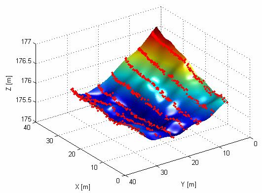
181 (a) (b) 161

182 (c) (d) 162

183 (e) (f) Figure 5.9. Modeled LiDAR surfaces The main trend of the surfaces was modeled by a polynomial, properly choosing the polynomial order based on the complexity of the trend. The fundamental frequencies of 163