DISCRETE EVENT SYSTEM MODELING USING SYSML AND MODEL TRANSFORMATION

Transcription

1 DISCRETE EVENT SYSTEM MODELING USING SYSML AND MODEL TRANSFORMATION A Dissertation Presented to The Academic Faculty by Chien-Chung Huang In Partial Fulfillment of the Requirements for the Degree Doctor of Philosophy in the School of Industrial and Systems Engineering Georgia Institute of Technology December 2011 COPYRIGHT 2011 BY CHIEN-CHUNG HUANG

2 DISCRETE EVENT SYSTEM MODELING USING SYSML AND MODEL TRANSFORMATION Approved by: Dr. Leon F. McGinnis, Advisor School of Industrial and Systems Engineering Georgia Institute of Technology Dr. Christos Alexopoulos School of Industrial and Systems Engineering Georgia Institute of Technology Dr. Chris Paredis School of Mechanical Engineering Georgia Institute of Technology Dr. Chen Zhou School of Industrial and Systems Engineering Georgia Institute of Technology Dr. Marc Goetschalckx School of Industrial and Systems Engineering Georgia Institute of Technology Date Approved: [August 18, 2011]

3 To Emily, for her encouragement and support. iii

4 ACKNOWLEDGEMENTS I offer my sincere thanks to many people who helped me accomplish the completion of my doctoral degree. First of all, I would like to express my sincere gratitude to my advisor, Dr. Leon McGinnis. I especially thank him for providing me with lots of professional advice, teaching me how to be a better researcher, and supporting and encouraging me. Because of him, I am able to overcome many challenges during the PhD process. I also offer my sincere appreciation to Dr. Chris Paredis, who was always very kind and patient in answering my questions about this research. Deep thanks also are extended to Dr. Christos Alexopoulos, Dr. Chen Zhou, and Dr. Marc Goetschalckx, who gave me many professional ideas and stimulated my thinking in different ways so that I could improve the quality and content of my research study. This dissertation would not have been possible without all the assistance I have received. In addition, a special acknowledgment goes to my lab mates, including but not limited to Dr. Kan Wu, Kysang Kwon, Randeep Ramamurthy, George Thiers, Dr. Volkan Ustun, and Dr. Ola Batarseh, who always discuss with me and enhance my understanding of these topics. Finally, I want to express my deepest gratitude to my parents. They always provide love, encouragement, support, and help to me. Without them, it would have been impossible for me to study abroad, get a doctoral degree, and make my dream come true.. iv

5 TABLE OF CONTENTS ACKNOWLEDGEMENTS LIST OF TABLES LIST OF FIGURES LIST OF ABBREVIATIONS SUMMARY IV IX X XII XIII CHAPTER 1 INTRODUCTION Formal Languages Object-oriented Modeling Philosophy Problem Description and Research Objective Overview of the Thesis 6 CHAPTER 2 FORMAL LANGUAGES AND SYSML Background and Motivation Factors of Comparison Formal Languages for Discrete Event Systems Logical Languages Moore Machine Mealy Machine Petri Net IDEF Discrete Event System Specification (DEVS) Unified Modeling Language (UML) System Modeling Language (SysML) Comparison between Conceptual Modeling Languages Summary 41 CHAPTER 3 DISCRETE EVENT SYSTEM MODELING PROCESS USING SYSML Background and Motivation Definition of Discrete Event Systems Object-Oriented Modeling Process for Discrete Event Systems State Explosion Problem Description Top-down Approach Bottom-up Approach 50 v

6 3.4.4 Parametric Approach Discrete Event Modeling Process Top-down Approach Using SysML Bottom-up Approach in SysML Parametric Approach in SysML Subset of SysML for DES Proposed Modeling Process in SysML Conclusion 60 CHAPTER 4 THE GENERIC SYSML SUBSET Introduction Literature Review Formal Definition of Object-oriented Models Automata Theory Formal Definition of the Proposed SysML Subset System Structure of the Proposed SysML Subset System Behavior of the Proposed SysML Subset The Transformation relationship between the system model and the decomposed model The Relationship between System Models and Decomposed Models Transformation Algorithm from Decomposed Models to System Models Transformation Algorithm from System Models to Decomposed Models Example of the Proposed Transformation Algorithm The Interchangeability between System Models and Decomposed Models Conclusion 92 CHAPTER 5 RELATIONSHIP BETWEEN CONCEPTUAL MODELING LANGUAGES Introduction Transformations between State-based Modeling Languages Logical Language and Automata Harel Statechart and UML/SysML State Machine Diagram Mealy Machine and Moore Machine Relationship between State Machine Diagrams, Moore and Mealy Machines State-based Modeling Language Relationships Conclusion 106 CHAPTER 6 USING PETRI NETS TO VERIFY CONTROL MODELS SPECIFIED AS ACTIVITY DIAGRAMS Introduction Control Modeling in Petri Nets and UML/SysML Petri Nets UML/SysML Syntax and Execution Semantics of Petri nets and Activity Diagrams 112 vi

7 6.3.1 Syntax of Petri Nets Syntax of UML/SysML Activity Diagrams Execution Semantics of Petri Nets and Activity Diagrams Mapping Rules Act-to-PN Transformation Algorithm Valid PN ACT-to-PN Transformation Algorithm Equivalence Properties Equivalence Properties for Valid PN Equivalence Properties for Invalid PN Implementation Example Tutorial Model Control Model of Fractal Manufacturing Systems Conclusion 134 CHAPTER 7 AUTOMATING SIMULATION OF CONTROL MODELS EXPRESSED AS UML/SYSML ACTIVITY DIAGRAMS Introduction Literature Review Control Model Transformation Executable UML The Proposed Transformation the Tree Structure Proposed Intermediate Meta-model Formal Definition of Activity Diagrams Transformation from an Activity Diagram to a Parse-tree Transformation from the Proposed Tree Structure to the Simulation Code Transformation Example and Implementation Detail Example of Control Transformation Conclusion 158 CHAPTER 8 MODEL TRANSFORMATION USING LIBRARIES AS DOMAIN SPECIFIC LANGUAGES Introduction Literature review Transformation Procedure Model Transformation Technology OMG Four-layer Meta-modeling Architecture Model Transformation Framework- Using Libraries as Domain Specific Language Concept of Model Transformation SysML Meta-model AnyLogic Meta-model Mapping rules of the Transformation Transformation Procedure 172 vii

8 8.5 Demonstration Conclusion and Future Research 175 CHAPTER 9 CONCLUSIONS Summary and Conclusions Future Research 179 REFERENCES 180 VITA 190 viii

9 LIST OF TABLES Table 1: Some attributes of languages, formal languages and formal systems... 4 Table 2: The summarized table for the conceptual modeling languages Table 3: The comparison of the structure diagrams in the conceptual modeling languages Table 4: The comparison of the behavior diagrams in the conceptual modeling languages Table 5: The number of system states Table 6: The comparison between system states and decomposed states Table 7: The structure tuple of the blocks Table 8: The automata of a decomposed model Table 9: Mapping rules for load-and-send nodes without execution durations Table 10: Mapping rules for action nodes with execution durations Table 11: Mapping rules for immediate-repeat nodes Table 12: Activity tuple of the tutorial example Table 13: Petri net tuple of the tutorial example in the second step Table 14: Petri net tuple of the tutorial example in the third step Table 15: Corresponding Petri net tuple of the tutorial example Table 16: Mapping rules between the tree node and simulation language Table 17: Computational results for the bucket manufacturing process ix

10 LIST OF FIGURES Figure 1: The relationship between conceptual model and simulation model [35] 3 Figure 2: Schematic diagram of a simple experiment based on [65] 14 Figure 3: A Moore machine example [62] 15 Figure 4: A Mealy machine example 18 Figure 5: Petri net example [67] 20 Figure 6: Example of IDEF0 [60] 23 Figure 7: Example of IDEF4 [60] 24 Figure 8: Example of UML class diagram 31 Figure 9: Example of UML sequence diagram 32 Figure 10: Example of UML state machine diagram 33 Figure 11: Example of UML activity diagram 33 Figure 12: SysML Diagram Taxonomy [4] 35 Figure 13: Example of Block Definition Diagram 36 Figure 14: Example of Internal Block Diagram 37 Figure 15: A discrete event system [77] 45 Figure 16: Object-oriented modeling methodology for manufacturing information systems modified from [49] 46 Figure 17: Example of a hierarchical state machine 49 Figure 18: The corresponding state machine 50 Figure 19: Example of an assembly line 51 Figure 20: The state diagram of B1 52 Figure 21: The state diagram of B1 using parameter approach 54 Figure 22: BDD of the assembly line example 58 Figure 23: IBD of the assembly line system 59 Figure 24: State machine diagrams of the buffer and machine 59 Figure 25: The concept of the behavior modeling using SysML 60 Figure 26: SysML example (B1 and B2) 76 Figure 27: SysML example (B1 and B3) 77 Figure 28: The system model of the example with one buffer and one machine 86 Figure 29: The decomposed model of the example without actions 88 Figure 30: The decomposed model of the example 88 Figure 31: The finite state machine of the example 89 Figure 32: A finite-state machine example 97 Figure 33: Example of SysML/UML state machine and Harel Statechart 98 Figure 34: Transformation example from Moore machine to Mealy machine 101 Figure 35: Transformation example from Mealy machine to Moore machine 103 Figure 36: The overall picture of the conceptual modeling language relationship 106 Figure 37: (a) An example of the activity diagram. (b) The corresponding PN of the example. 110 Figure 38: (a) A two-action example of the activity diagram; (b) A two-action example with pins; (c) The corresponding PN diagram. 120 Figure 39: A tutorial case of control modeling using activity diagrams. 130 Figure 40: PN constructed from the tutorial activity diagram. 132 Figure 41: An activity diagram of DMA. 133 Figure 42: The corresponding PN diagram of DMA. 134 x

11 Figure 43: Example of control modeling using activity diagrams. 137 Figure 44: Concept of foundational UML based on [3]. 140 Figure 45: Example of parse-tree based on [74]. 142 Figure 46: Example of the proposed tree structure. 143 Figure 47: (a) Example of a cyclic activity diagram. (b) The equivalent acyclic activity diagram. 147 Figure 48: (a) Example of the activity nodes with multiple input edges. (b) The equivalent tree structure. 149 Figure 49: Generated Pseudo code of the example in Figure 47(a). 151 Figure 50: Example of a control model using UML/SysML activity diagrams. 151 Figure 51: Corresponding Pseudo code in SimTalk. 152 Figure 52: Tree structure of the control model. 153 Figure 53: Bucket manufacturing process. 154 Figure 54: Pull-based release rule. 155 Figure 55: Tree structure of the pull-based release rule. 155 Figure 56: Generated simulation script of the pull-based release rule. 156 Figure 57: Bucket manufacturing process in Plant Simulation. 157 Figure 58: Interpretation across meta-layers [3]. 164 Figure 59: SysML meta-model for BDD. 166 Figure 60: SysML meta-model for IBD. 166 Figure 61: SysML meta-model for SM. 167 Figure 62: SysML meta-model for ACT. 167 Figure 63: AnyLogic meta-model. 168 Figure 64: AnyLogic meta-model. 168 Figure 65: AnyLogic meta-model. 169 Figure 66: AnyLogic meta-model. 169 Figure 67: Partial mapping rules. 170 Figure 68: Partial mapping rules. 171 Figure 69: Partial mapping rules. 171 Figure 70: Partial mapping rules. 171 Figure 71: Partial structure of the machine library. 173 Figure 72: Partial behavior of the machine library. 174 Figure 73: Generated AnyLogic project. 174 Figure 74: Partial generated AnyLogic project file. 175 xi

12 LIST OF ABBREVIATIONS ACT BDD COTS CPN DELS DES DEVS FSM IBD IDEF MOF MPSG OO PN SD SM SysML UML XMI Activity Diagram Block Definition Diagram Commercial-Off-The-Shelf Colored Petri Net Discrete Event Logistics Systems Discrete Event System Discrete Event System Specification Finite State Machine Internal Block Diagram Integration DEFinition Meta-Object Facility Message-based Part State Graph Object-Oriented Petri Net Sequence Diagram State Machine Diagram System Modeling Language Unified Modeling Language XML Metadata Interchange xii

13 SUMMARY The objective of this dissertation is to introduce a unified framework for modeling and simulating discrete event logistics systems (DELS) by using a formal language, the System Modeling Language (SysML), for conceptual modeling and a corresponding methodology for translating the conceptual model into a simulation model. There are three parts in this research: plant modeling, control modeling, and simulation generation. Plant Modeling of Discrete Event Logistics Systems Contemporary DELS are complex and challenging to design. One challenge is to describe the system in a formal language. We propose a unified framework for modeling DELS using SysML. A SysML subset for plant modeling is identified in this research. We show that any system can be described by using the proposed subset if the system can be modeled using finite state machines or finite state automata. Furthermore, the system modeled by the proposed subset can avoid the state explosion problem, i.e., the number of the system states grows exponentially when the number of the components increases. We also compare this approach to other existing modeling languages. Control Modeling of Discrete Event Logistics Systems The development of contemporary manufacturing control systems is an extremely complex process. One approach for modeling control systems uses activity diagrams from SysML, providing a standard object-oriented graphical notation and enhancing reusability. However, SysML activity diagrams do not directly support the kind of analysis needed to verify the control model, such as might be available with a Petri net (PN) model. We show that a control model represented by UML/SysML activity xiii

14 diagrams can be transformed into an equivalent PN, so the analysis capability of PN can be used and the results applied back in the activity diagram model. We define a formal mathematical notation for activity diagrams, show the mapping rules between PN and activity diagrams, and propose a formal transformation algorithm. Discrete Event Simulation Generation The challenge of cost-effectively creating discrete event simulation models is well-known. One approach to alleviate this issue is to describe a system using a descriptive modeling language and then transform the system model to a simulation model. Some researchers have tried to realize this idea using a transformation script. However, most of the transformation approaches depend on a domain specific language, so extending the domain specific language may require modifying the transformation script. We propose a transformation approach from SysML to a simulation language. We show that a transformation script can be independent of the associated domain specific language if the domain specific language is implemented as domain libraries using a proposed SysML subset. In this case, both the domain library and the system model can be transformed to a target simulation language. We demonstrate a proof-of-concept example using AnyLogic as the target simulation language. xiv

15 CHAPTER 1 INTRODUCTION A discrete event logistics system (DELS) is a dynamic system that evolves in accordance with the occurrence, at possibly unknown irregular intervals, of events associated with material flow [77]. DELS are an essential component of modern society, and represent a significant portion of global economic activity. They also present significant challenges in both analysis and design, because of their stochastic patterns, complicated correlations between state variables, non-stationary, non-renewal behaviors or complex state- and criterion-dependent control rules. Discrete event simulation models are widely used to analyze DELS because there are no other high-fidelity analysis approaches that can cope with these systems in their full complexity. Discrete event simulation models are enabled by a wide range of commercial-off-the-shelf (COTS) tools. However, modeling large-scale DELS and creating their simulation models is not without challenges. Although there are many COTS tools which provide drag-and-drop functionality to author simulation models, it s still difficult to reliably create a valid high fidelity model for a large complex system. For the DELS domain expert, the simulation model is a black box so validating that the simulation model accurately reproduces the behavior of the target system is a difficult task. One consequence is that, in contemporary practice, large scale simulation is time-consuming and expensive. There are two distinct phases involved in constructing a DELS simulation: developing a conceptual model of the target DELS and developing the actual (computational) simulation model. The conceptual model is an abstract representation of the target system, and reflects the requirements for the simulation model. A conceptual model has a particular purpose, i.e., it is intended to answer a specific question or set of 1

16 questions. The conceptual model describes the characteristics of the system. There are many approaches to authoring explicit conceptual models such as mathematics, text descriptions or graphic representations; the conceptual model also may be implicit, i.e., not recorded. A simulation model is a computational implementation of a conceptual model, which produces data representing the time-based and the event-based behavior of the target system. There is a broad range of simulation languages and specific simulation tools. Some of the tools provide for real-time user interaction or visual animations, and all require deep knowledge in order to create high fidelity models of large scale DELS. Thus, DELS domain experts are rarely ever sufficiently expert in simulation methods and tools to be able to do the DELS simulation modeling themselves, and as a consequence, the domain experts must try to communicate a conceptual model to the simulation experts who do the actual simulation modeling. The target system is abstracted to the conceptual model. The simulation model is created from the description contained in the conceptual model and implements this description in a computational form using simulation software. The relationship between the conceptual model and the simulation model is shown in Figure 1. Two reasons to construct an explicit conceptual model are: (1) to capture a target system description that can be validated with the problem owner ; and (2) to provide a well documented basis for the simulation expert to use in constructing the computational simulation. 2

17 Figure 1: The relationship between conceptual model and simulation model [35] The conceptual model is a critical link between the target system and the simulation model. For large, complex systems, such as DELS, the cost and quality of the simulation model (and its results) are directly related to the fidelity of the conceptual model if it is not accurate, or it fails to include important problem characteristics, the corresponding simulation model will fail to accurately portray the target system behavior. The lack of specific tools or methods for conceptual modeling belies its importance in DELS simulation. A fundamental goal of this dissertation is to establish a formal approach to DELS conceptual modeling by using formal languages. 1.1 Formal Languages Mateescu and Salomaa [59] define a language and formal language as follows: A language is a set of finite strings of symbols from a finite alphabet. Depending on the context, the finite strings constituting a language can also be referred to as words, sentences, programs, etc. When speaking of formal languages, we want to construct formal grammars for defining languages rather than to consider a language as a body of words 3

18 somehow given to us or common to a group of people. Formal grammars will be devices for defining specific languages. One example of formal language is arithmetic. The alphabet includes number symbols and arithmetical operation symbols. Words are either strings of numbers or single arithmetic operation. One grammar rule requires the words to the left and right of an arithmetic operation symbol must be a number string. Based on these definitions, the string = 46 is valid but not the string = A formal system is a subtype of a formal language. Herre and Heister [43] define formal systems in this way: Formal systems are formal languages equipped with a consequence operation yielding a deductive system. The consequence operations are the inductive rules or axioms. Elementary algebra is an example of a formal system. The commutative operation ( y + z = z + y ) and the substitution operation ( w = x + y w + z = x + y + z ) are inductive rules. These rules imply that the string ( x + y + z = z + x + y ) and the string ( x + y + z = y + z + x ) also are valid. These strings can be captured in operations of a formal system instead of describing one by one in formal languages. The differences between languages, formal languages, and formal systems are summarized in Table 1. Grammars to validate sentences are required in formal languages, but not in languages. Consequence operations are required in formal systems. Table 1: Some attributes of languages, formal languages and formal systems Languages Formal languages Formal Systems A finite alphabet Grammar Consequence operations 4

19 1.2 Object-oriented Modeling Philosophy One category of formal languages is object-oriented languages, which are the languages supporting object-oriented concepts. Object-oriented concepts describe the target system by using classes and instances. An instance represents a corresponding component in the target system. A class is a blueprint for similar instances. For example, the general description of a dog is captured in a class and a specific dog is an instance of the dog class, e.g., the dog named Spot. Many researchers propose using object-oriented (OO) languages to create conceptual models. Compared to non-oo languages, OO languages afford a number of advantages. Object-oriented concepts such as inheritance relationships, which mean the source class is a sub-type of the target classes, are inductive rules. If A inherits from B and B inherits from C, it also is true that A inherits from C. Because of these operations, an object-oriented modeling language also may be a formal system. Another advantage of object-oriented concepts is enabling reusability, modifiability and maintainability [96]. Object-oriented concepts can reuse the same description for all instances, i.e. all of the job with the same product type may have the same description. When a property of the class is changed, the same property is modified in all the corresponding instances. Finally, using object-oriented concepts, it is possible to have objects representing physical components in a real system [13]. Because of these advantages, Robinson [80] points out that one interest of the current simulation research is to use an object-oriented language as the conceptual modeling language and then generate the simulation model rather than create it from scratch. These advantages of object-oriented concepts may reduce the modeling complexity for DELS conceptual models. However, the lack of a unified framework for using an object-oriented language as a formal DELS conceptual modeling language makes it difficult to realize these advantages especially for a complex, large-scale DELS. 5

20 1.3 Problem Description and Research Objective This research aims to create a unified framework for modeling and simulating large-scale DELS by defining a formal language for conceptual modeling and a corresponding methodology for translating the conceptual model into a specific simulation model. There are three distinct contributions of this research. The first contribution is the unified framework for modeling large-scale DELS by applying object-oriented languages. In the literature, some frameworks using objectoriented concepts have been discussed but few of them are used for DELS. The goal is to develop a generic and formal framework using object-oriented languages for DELS and to compare to other existing conceptual modeling languages. The second contribution is the control modeling of DELS. Control is especially critical in the discrete-event manufacturing environment. A new object-oriented and graphical representation for modeling control will be proposed, demonstrated, and evaluated. The third contribution is the proof of concept that a large, complex DELS simulation model can be generated from its high-fidelity conceptual model. Creating a large scale simulation is usually time-consuming and expensive. Instead of directly creating the simulation model, the proof of concept will demonstrate a transformation method that will use the specific conceptual model and produce its corresponding simulation model. 1.4 Overview of the Thesis The main focus of this thesis is DELS. Since DELS are a type of discrete event system (DES), the existing conceptual modeling languages for DES and their relationships to the proposed modeling language is the focus of Part I (from Chapter 2 to Chapter 5). Part I is organized as follows: In order to describe conceptual models formally, formal languages used in modeling DES are reviewed and compared in Chapter 2. In Chapter 3, the 6

21 modeling principals of the general discrete event system and an object-oriented modeling process are presented. In Chapter 4, we propose a transformation algorithm between one formal language, finite-state automata, and the proposed modeling language. Chapter 5 contains the relationships between the proposed modeling language and other conceptual modeling languages such as Moore machines, Mealy machines, and logical languages. Part II (Chapters 6 and 7) of this dissertation addresses control modeling, which is critical in DELS. In Chapter 6, we focus on DELS in which the control modeling is important. The control modeling in the literature is reviewed and a control modeling framework is proposed and demonstrated. In Chapter 7, we discuss the transformation of the control logic from the proposed control modeling framework to simulation models. The language used to describe control logic may be different from the simulation languages. Thus transformation is required to generate the executable simulation model. The last part (Chapter 8) shows the proof of concept that that a large, complex DELS simulation model can be generated from its high-fidelity conceptual model. We present a transformation algorithm including not only the control logic but also the structure and the behavior of the system from the conceptual model to the simulation model. We end up the conclusion and discuss possible direction for future research in Chapter 9. 7

22 CHAPTER 2 FORMAL LANGUAGES AND SYSML 2.1 Background and Motivation Modeling a large-scale discrete event logistic system (DELS) is not without challenges. One challenge is to describe the system in a formal way. In practice, the domain experts create conceptual models in their authoring tools such as AutoCAD, FactoryCAD or some spreadsheet files. Because these languages are not formal, it is possible that the conceptual model will not be perfectly understood by the simulation experts who must use it as the basis for creating the simulation model. One approach to solving this problem is to replace these informal languages with a formal language. Formal languages can be used to create formal conceptual models. A formal language is normally defined by an alphabet and its grammars. An alphabet is a set of symbols used to construct sentences and grammars are the rules to validate these sentences. The alphabet and grammar are defined in a formal language so that other stakeholders can understand the descriptions. Many formal languages have been proposed in the past three decades to describe discrete event systems (DES), which includes DELS. Some examples are Moore machine [65], Mealy machine [62], Petri nets [72], Integration DEFinition (IDEF) [1], Discrete Event System Specification (DEVs) [101], UML [5] and SysML [4]. Since a large-scale DELS may involve thousands of entities, some requirements for a conceptual modeling language are important. One requirement is model reusability, i.e. how a description created once can be re-used for similar problems. Another requirement is support for hierarchical modeling or graphical representations so that the development of large conceptual models can be managed effectively, and they can be understood easily by a range of stakeholders. However, not all formal languages can 8

23 support these requirements. The comparison of candidate formal languages is required and addressed in this chapter. This chapter is organized as follows. In Section 2.2, we survey and select the important factors of formal languages for a large-scale DES. In Section 2.3, we review formal languages used for DES. In Section 2.4, we discuss the comparison between these formal languages and ends with conclusions. 2.2 Factors of Comparison There are a number of ways to classify conceptual modeling languages. Heavy and Ryan [41] identify two categories. One is the formal language with a formal method which has a formal basis and numerous software implementations. The other is the formal language with a descriptive method that has little formal basis and is primarily made up of software implementations. Formal languages with little formal basis usually have a descriptive specification, but do not provide precise meanings. Another classification is based on modeling techniques which the formal languages can support. Killich et al. [48] identify three modeling techniques which the formal languages can support: state-oriented techniques, event-oriented techniques and techniques based on Petri nets. State-oriented techniques describe a system by capturing all states. Event-oriented techniques focus on the sequence of events, the object flow or the information flow of the system. Petri nets are a special language which can support both state-oriented and event-oriented modeling techniques, e.g., a place in a Petri net can represent either a state or an object flow. The detail of Petri nets will be discussed in Section Support for object-oriented concepts is another potential comparison factor. Object-oriented concepts afford some advantages for creating conceptual models: enabling reusability, modifiability and maintainability [96]. Since a large-scale DES may 9

24 involve thousands of entities, and typically they can be grouped into classes, with similar descriptions for all entities in the same class, the reusability, modifiability or maintainability of these descriptions by classes may reduce the overall modeling complexity. Killich et. al. [48] compare formal languages by considering hierarchical modeling, layering mechanisms and purpose-driven views. A formal language supporting hierarchical modeling can decompose a component into its sub-components. Layering mechanisms provide a way to describe a system in an abstract model in the beginning and then elaborate to the more concrete model. Purpose-driven views support different views for the purpose of addressing a set of stakeholder concerns. The graphical representation and model understandability are also important for modeling a large-scale DES. Compared to a purely textual description, a formal language with a graphical representation affords a number of the advantages: raising the level of abstraction, reducing the amount of information to what is needed to perform the task at hand, and easing browsing the large information space [51]. These advantages may make it easier to share a descriptive model with stakeholders and for them to understand. Two other criteria of comparison between conceptual modeling languages are modeling verification and model simulation. Ryu and Yücesan [82] define model verification in formal languages as providing a formal basis to determine if the conceptual model is true, i.e. any contradiction in a model can be detected by verification rules. They also define model simulation in formal languages as providing capability for a conceptual model represented in the formal language to be simulated directly in a simulation tool. 10

25 2.3 Formal Languages for Discrete Event Systems There are two major categories of formal languages used in discrete event systems. One category is logical languages which do not include any time information. The other category includes languages which incorporate deterministic or stochastic time information [77]. In object-oriented concepts, classes capture blueprints of similar description so classes are usually described by a logical language. The related logical languages are reviewed in this research Logical Languages Description A logical language, L, is specified by its events and the set of all possible event sequences. The set of event types is denoted as Σ, and the set of all of the possible event sequences, or strings, denoted as Σ *. For example, a customer goes to a clinic. The events ( Σ ) of this example are customer arrival events (σ ), entering-waiting-line events (δ ), diagnosis events (κ ), and departure events (α ). strings. One example of an event string in * Σ is the set of all possible event * Σ is {σδκα }. Since the event sequences may have infinite length, these event sequences can not be modeled explicitly by listing the event sequences. A subset of logical languages can be modeled by using the prefix relationship if the language has a prefix closure language, defined as follows. The language L is the prefix closure language of the language L if and only if L * = { μ : μν L for some v Σ } and L = L. A string denoted as μ is the prefix of the string ω if there exists a string ν such that ω = μν. Based on this definition, the prefix can be any possible length from the 11

26 beginning of the given string ω. A logical language is a prefix closure language if all of the prefixes are also included in the logical language itself. Logical languages use their event labels and prefix closure to describe a discrete event system. For example, assume that the discrete event system has two independent events denoted as {a,b}. The event list is Σ = { ε, a, b} whereε is the empty string. L = L = { ε, a, b, ab, ba, aba...}. The waiting line of the clinic is another example. The number of the entering-to-the-waiting-line events is greater than or equal to the number of the diagnosed events. We denote w as the number of events of type e in the string e * w, μ is an event string, and then L = { w Σ : for each prefix μ of ω, u a u b } Logical languages provide a formal basis and are used to analyze all possible event sequences. However, most cases in the literature are small with fewer than 10 events. In addition, logical languages can be complicated since the number of possible event strings may be infinite. If the system has more than 4 event types and there exists some correlations between events, it is not easy to represent in a mathematical formulation. Furthermore, logical languages only represent events and their sequences, not the physical structure features of the system generating the events Comparison Factors Logical languages have the following attributes 1. Model type: Logical languages use mathematical formulations to describe all possible event sequences. According to Heavy and Ryan s definition [41], the mathematical formulations provide a formal basis and logical languages are formal languages with a formal method. 2. Modeling technique: Logical languages describe event sequences, so they can support event-oriented techniques. 12

27 3. Supporting Object-Oriented concepts: The definition of logical languages includes events and event sequences but logical languages do not support the definition of classes or instances. As a consequence, logical languages do not support object-oriented concepts. 4. Hierarchical, layering, and purpose-driven view: The definitions of logical languages do not support hierarchical, layering, and purpose-driven view. 5. Graphical representation: Logical languages can be described mathematically but do not support graphical representation. 6. Model understandability: From the domain expert perspective, the mathematical formulation is not easy to understand. 7. Standardization: The formulation of logical languages is a standard representation. 8. Model verification: One way to verify a model is to compare the event sequences between the modeler s understanding and the model represented by the logical language [78]. An event sequence can be verified if it exists in the sets of the logical language or does not violate any logical language definition. 9. Model simulation: Logical languages don t support simulation directly. 13

28 2.3.2 Moore Machine Description Moore [65] in 1956 analyzed the sequential machine shown in Figure 2. A sequential machine may have multiple states. When an input symbol is received, the state of this machine changes. Each state produces output symbols back to the experimenter. The typewriter is one example of a sequential machine. The input symbols are the input typing from the typist. The input symbols change the state of the typewriter from idle to typing and the output is a new character on the paper. The typist can observe the output symbol and make the next decision. Figure 2: Schematic diagram of a simple experiment based on [65] The main idea of the Moore machine is to abstract the sequential machine for which the output symbols are determined by the current state. A Moore machine has a finite set of states including an initial state, a finite set of input symbols, and a finite set of output symbols. State changes are defined by a transition function. In operation, the Moore machine is in some state; when an input symbol is received, it transitions to a new state (perhaps the same state), and produces an output symbol. Mathematically, a Moore machine M can be defined as a 6-tuple, M = { X, I, F, x0, O, G} where 14

29 X is a finite set of states I is a finite set of input events F is a finite set of transition functions and F : X I X x 0 is an initial state and x 0 O is a finite set of output events G is a finite set of output functions and X G : X O Figure 3 is a graphical representation of a specific Moore machine. The system has three states: X = q, q, }. The set of input events I is { 0,1} and the set of output { 1 2 q3 events O is { 0,1}. Each state has its own output function which is shown as F = { q1 0 q2, q1 1 q1, q2 0 q3, q2 1 q1, q3 0 q2, q3 1 q1}. The output function G is q 0, q 1, q 0} { Figure 3: A Moore machine example [62] Moore machines describe all of the states, events, and transitions. However, Moore machines can t represent physical components in a real system. In addition, the number of states in a large-scale model may be too large to be modeled explicitly Comparison Factors Moore machines have the following attributes: 15

30 1. Model type: Moore machines can be defined in a 6-tuple. Based on Heavy and Ryan s work, Moore machines are a formal language with a formal method. 2. Modeling technique: Moore machines capture the states and the state transitions, so Moore machines can support state-oriented techniques. 3. Supporting object-oriented concepts: The definition of Moore machines doesn t include classes and instances so Moore machines do not support object-oriented concepts. 4. Hierarchical, layering, and purpose-driven view: Moore machines do not support hierarchical, layering, and purpose-driven view. 5. Graphical representation: Moore machines can be represented graphically by using the state charts including all states, events and transitions. However, there is no formal definition of the graphical representation for Moore Machines. 6. Model understandability: From the domain expert perspective, the tuple representation is not easy to understand. Furthermore, for a large-scale model, the number of states may be too large to be modeled explicitly which can not be understood easily. 7. Standardization: The 6-tuple is a standard representation. 8. Model verification: A model represented by Moore machines is verified if there is no contradiction. One example of a contradiction is that two transition functions have the same states, and input events, but have different output states. 9. Model simulation: Moore machines don t support simulation directly. 16

31 2.3.3 Mealy Machines Description Mealy [62] proposed Mealy Machines in A Mealy machine is a sequential machine, but has different output functions than a Moore machine. In Moore machines, output functions are dependent on the current state and return the output events. The output functions in Mealy machines consider not only the current state but also the input event. A Mealy machine can be represented in a six-tuple. M = { X, I, F, x0, O, G} Where X is a finite set of states I is a finite set of input events F is a finite set of transition functions and F : X I X x 0 is an initial state and x 0 O is a finite set of output events X G is a finite set of output functions and G : X I O One example of a conceptual model represented by a Mealy machine is shown in Figure 4. This discrete event system has three states represented as X = { S1, S2, S3}, two input events represented as I = { e1, e2}, six output events represented as O = {A1, A 2, A3, A4, A5, A6}, six transition functions represented as F = { S1 e1 S2, S1 e2 S3, S2 e1 S3, S2 e2 S1, S3 e1 S1, S3 e2 S2} and six output functions represented as G = { S1 e1 A1, S1 e2 A2, S2 e1 A5, S2 e2 A3, S3 e1 A4, S3 e2 A6}. The difference between Moore machines and Mealy machines is the output function. The output function in Moore machines is determined by 17

32 the current state, but the output function in Mealy machines is determined by both the current state and input events. Figure 4: A Mealy machine example The elements in Mealy machines describe states, events and transition functions. However, Mealy machines can t represent physical components in a real system. Thus, Mealy machines don t support object-oriented concepts for modeling complete systems Comparison Factors Mealy machines have the following attributes: 1. Model type: Mealy machines can be defined in a 6-tuple. Based on Heavy and Ryan s work, Mealy machines are a formal language with a formal method. 2. Modeling technique: Mealy machines capture the states and the state transitions, so Mealy machines can support state-oriented techniques. 3. Supporting object-oriented concepts: The definition of Mealy machines doesn t include classes and instance so Mealy machines do not support objectoriented concepts. 18

33 4. Hierarchical, layering, and purpose-driven view: Mealy machines do not support hierarchical, layering, and purpose-driven view. 5. Graphical representation: Mealy machines can be represented graphically by using the state charts including all states, events and transitions. However, there is no formal definition of the graphical representation for Mealy Machines. 6. Model understandability: From the domain expert perspective, the tuple representation is not easy to understand. Furthermore, for a large-scale model, the number of states may be too large to be modeled explicitly which can not be understood easily. 7. Standardization: The 6-tuple is a standard representation. 8. Model verification: A model represented by Mealy machines is verified if there is no contradiction, e.g. two transition functions have the same input states, input events, but have different output states. 9. Model simulation: Mealy machines don t support simulation directly Petri Net Description The original Petri net was developed by Petri [72] in A Petri net (PN) is a directed bipartite graph with transitions, places and directed arcs as illustrated in Figure 5. PNs are executed by using tokens that may pass through the system. The places represented by the circles may contain one or more tokens. The transitions represented by the bars fire the events. The arcs connect a transition to a place or a place to a transition. For any transition, the places with an arc into a transition are called the input places of the transition, and the places with an arc from the transition are called the output 19

34 places.when all input places to a transition have at least one token, this transition is fired. After it fires, one token is consumed from each input place of this transition and one token is added to all of the output places. A Petri net graph PN can be represented by a three-tuple. PN = { P, T, A} Where P is a finite set of places T is a finite set of transitions A is a finite set of arcs and A ( P T) ( T P) Figure 5 shows a conceptual model represented by Petri nets. The places are denoted from P 1 to P 6. P = { P1, P2, P3, P4, P5, P6 } The transitions are the bars from t 1 to t 5. T = { t1, t2, t3, t4, t5}. The arcs A are {( P 1 t1), ( P1 t2), ( P2 t3), ( P3 t3), ( P4 t4), ( P5 t4), P t ), ( t P ), ( t P ), ( t P ),( t P ), ( t P ), ( t )}.In the first step, the token ( P1 in P 4 won t trigger t 4 because there are no tokens in P 5. P 1 can trigger t 1 or t 2. If t 2 is fired, the token in P 1 is consumed and another token is placed in P 5. After this step, all of the input places to t 4 have at least one token, and t 4 is triggered. Figure 5: Petri net example [67] 20

35 There are some variations of Petri net. Moore and Gupta [66] classify the temporal Petri net as two major classes: timed Petri nets and stochastic Petri nets. Timed Petri nets are Petri nets with deterministic transition times; Stochastic Petri nets are Petri net with random transition times. Another variation is colored Petri nets (CPNs). CPNs provide a method for distinguishing between token types by allowing a token type to have its own attributes or data structure [66]. A recent development of the Petri net is the objected-oriented Petri net framework. Lee and Park [53] propose an object-oriented high-level Petri net for realtime system modeling. They define a new element, system, which is composed of mutually communicating hierarchical systems and their interconnection relations. Each system contains its own Petri net. The communications between related objects are supported by a set of interconnection relations which provide message-passing among related systems. The concept of the system is the similar to the concept of the class in object-oriented concept so each system can be used simultaneously in several usages. Wang [95] extends the concept and uses Petri nets to model an automated manufacturing system. Applying object-oriented concepts to Petri nets can reduce some complexity of the Petri net models. However, a Petri net itself is not an object-oriented modeling language. In summary, Petri nets are very popular and powerful methods for the modeling and analysis of systems which exhibit parallelism, synchronization, non-determinism and resource sharing features [28]. Petri nets are also graphical and formal modeling tools. However, from the conceptual modeling perspective, their use is difficult due to the complexity of the techniques [42]. Petri nets are not capable of visually accounting for complex branching logic or hierarchically decomposing complex models into sub modes and as a result become cumbersome as system complexity increases [41]. 21

36 Comparison Factors Petri nets are analyzed by using the following factors: 1. Model type: Petri nets have an exact mathematical definition of their execution semantics. Based on Heavy and Ryan s work, Petri nets are a formal language with a formal method. 2. Modeling technique: Killich et al. [48] identify Petri nets as a special type of modeling technique, neither state-oriented nor event-oriented modeling language. 3. Supporting object-oriented concepts: There are some object-oriented Petri net frameworks which define new elements like system. However, Petri net itself is not an object-oriented language. 4. Hierarchical, layering, and purpose-driven view: Petri nets provide a hierarchical modeling, but not layering or purpose-driven view [48]. 5. Graphical representation: The Petri net models can be shown in a graphical representation. 6. Model understandability: Ryu and Yucesan [82] discuss the factor of model understandability. When the target system is large or complicated, the Petri net model may have many places or transitions in a diagram. Each place may represent a physical structure, a state, or a resource, making the model hard to understand. 7. Standardization: The basic definition of Petri net is well-defined but there are many different versions [82]. 8. Model verification: Petri nets provide properties for model verification like the rule to avoid deadlocks. 9. Model simulation: There are tools such as JARP [10] and HPSim [7] which can be used to simulate Petri nets directly. 22

37 2.3.5 IDEF Description IDEF (Integration DEFinition) is a family of graphical modeling languages and methodologies in the system and software domain. IDEF0 is for functional modeling, IDEF1 is for information modeling, especially for database design, IDEF2 is for simulation modeling, and IDEF4 is for object-oriented design. In this section, we introduce the related diagrams, IDEF0 and IDEF4. Figure 6 shows the concept of IDEF0. Each block represents a function. The upper arc represents control flow. The left arc represents the input to the function. The right arc represents the output of the function which may link to other functions. The mechanism arc represents needed resources. The modeling methodology of IDEF0 defines the scope of a system by using a top-down modeling approach. For example, a function may be composed of multiple component functions. This building block can be decomposed into a sub-idef0 diagram to show the detail function flow between component functions. Figure 6: Example of IDEF0 [60] 23

38 Cheng-Leong et al. [23] use IDEF for modeling manufacturing enterprise systems. Each diagram is a different view of the enterprise system. This approach is easy to understand and all diagrams are in the same framework. However, most diagrams used in the framework are not object-oriented. IDEF4 is an object-oriented modeling language as illustrated in Figure 7. In object-oriented language, a class is a construct, which is a blueprint to create similar objects and is shown as a block in the diagram. The first compartment shows the public features that all classes can access, and the second shows the private features that the class itself can access. A feature is an attribute, e.g. the color of a car is a feature of the car class. The last compartment is the name of the class. Inheritance relationships, which target classes are sub-types of parent classes, are represented by arcs. Figure 7: Example of IDEF4 [60] In general, IDEF is a descriptive language for conceptual models. While IDEF4 is an object-oriented modeling language, it is focused on the system structure and not system behavior. IDEF offers a means of representing complex system branching logic along with a means of hierarchically decomposing a model into related sub models [41]. One limitation of IDEF is the lack of coupling relationships between different types of 24

39 diagrams. IDEF4 is the only diagram which can apply object-oriented concepts, but IDEF4 focuses only on the structure of the system Comparison Factors IDEF is analyzed by using the following factors: 1. Model type: Based on Heavy and Ryan s work, IDEF is a formal language with a descriptive method. 2. Modeling technique: The basic elements in IDEF0 are functions that are triggered by input events, so Killich et al. [48] classify IDEF as a eventoriented modeling language. 3. Supporting Object-Oriented concepts: IDEF only partially supports the Object-Oriented concepts. 4. Hierarchical, layering, and purpose-driven view: IDEF0 provides the hierarchical modeling mechanism. The top level function can be decomposed into a lower-level diagram [48]. IDEF does not support layering and purposedriven view. 5. Graphical representation: All IDEF diagrams are graphical representations. 6. Model understandability: The purpose of IDEF is to understand the system being modeled easily, so Ryu and Yucesan [82] classify IDEF as good on model understandability. 7. Standardization: Each diagram in IDEF has a standard definition [82]. 8. Model verification: IDEF doesn t provide tools or rules to verify a model. 9. Model simulation: The diagrams in IDEF can t be simulated directly. 25

40 2.3.6 Discrete Event System Specification (DEVS) Description Discrete Event System Specification (DEVS) is a modeling and analysis language for discrete event systems. Zeigler [101] proposed the DEVS-Scheme to support building models in a hierarchical, modular manner. In his view, a system has a time base, inputs, states, outputs, and functions for determining the next states and outputs, given current states and inputs. A basic DEVS model is called an atomic model. DEVS extends from the Moore machine model, in which the output action is associated with the state. An atomic model contains a set of external received events, external sent events, states and internal transition function which is executed itself after some time, the external transition function triggered by the events, the output function and the time advance function. An atomic DEVS model M a can be defined as a 7-tuple, M a = { X,, Y, δ in, δ ext, λ, ta} Where X is a finite set of input events Y is a finite set of output events is a finite set of states δ is a finite set of internal transition functions and δ : in δ is a finite set of external transition functions and δ X which ext t e is the elapsed time since the last event λ is a finite set of output functions and λ : Y t : R + is a time advance function a The differences between Moore machines and DEVS are the internal transition functions and time advanced functions. In DEVS, an internal transition represents a state in ext : t e 26

41 change if the state change is triggered after the lifespan of the original state, which is represented in the time advanced function. For example, the state of a doctor may change from busy to idle after the diagnosis time. This state change is an internal transition function and the diagnosis time is the time advanced function. The execution of an atomic model is as follows: The atomic model starts in some initial state. If there is no external event during the time advance period, the internal transition function is triggered and the output function of the state will be produced. If external events are received, the state will change, based on the external transition function. A coupled model may contain atomic models as sub-components. A coupled model has not only the coupling from external event to its sub-components but also the coupling relationship between sub-components. A coupled model may contain other coupled models and can be used to compose a system. A coupled DEVS model M c = where { X, Y, D, M, E, E, I, S} IC M c can be defined as a 8-tuple, OC X is a finite set of input events Y is a finite set of output events C D is a finite set of sub-components which can be DEVS atomic models or other coupled models M is a finite set of all sub-components and M = { M d d D} E is a finite set of external input couplings and E IC : X X i IC OC i D E is a finite set of external output couplings and E : Y Y I C is a finite set of internal couplings and I C : Y i D i OC i i D i D X i 27

42 S is a selection function which defines how to select the next event from simultaneous events. DEVS is capable of representing a system using a mathematic formulation which includes the structure of the target system and its states, but there is no graphical representation for a DEVS model. For a large-scale DES, it may be difficult for different stakeholders to understand the corresponding DEVS model. Heavey and Ryan [41] discussed DEVS as follows: The DEVS formalism is capable of accurately representing the various changes in state of a discrete event system along with being somewhat capable of representing resources, activities and branching within its mathematical representation. However the formalism is not visual in nature and does not account for the user s interactions with the system, information flows or a user friendly elaboration language. For a complicated system, a graphical representation can be important for verifying the fidelity of a conceptual model. Compared to the mathematical representation, the graphical representation may make it easier to share and communicate the domain knowledge between the domain expert and the modeling expert Comparison Factors DEVS has the following attributes: 1. Model type: DEVS can be defined by a mathematical formulation. Based on Heavy and Ryan s work, DEVS is a formal language with a formal method. 2. Modeling technique: DEVS captures the states of the target system, so DEVS are state-oriented modeling languages. 3. Supporting Object-Oriented concepts: DEVS doesn t support the definition of classes or instances, so DEVS doesn t support Object-Oriented concepts. 28

43 4. Hierarchical, layering, and purpose-driven view: DEVS provides the hierarchical modeling mechanism by using coupling models, but not for layering or purpose-driven view. 5. Graphical representation: DEVS models lack a graphical representation. 6. Model understandability: Each model in DEVS is represented as a mathematical tuple, and this is not easy to understand. 7. Standardization: DEVS has a standard definition by using a tuple. 8. Model verification: DEVS can be verified directly. 9. Model simulation: The models represented by DEVS can be simulated directly Unified Modeling Language (UML) Description UML (Unified modeling language) is an object-oriented modeling language that provides industry standard mechanisms for visualizing, specifying, constructing, and documenting software systems [30]. The objective of UML is to provide system architects, software engineers, and software developers with tools for analysis, design, and implementation of software-based systems as well as for modeling business process and similar workflows [5]. In UML 2.0, there are 13 types of diagrams which are used to model not only the static but also the dynamic aspects of systems. Class diagrams, sequence diagrams, activity diagrams and state machine diagrams are the diagrams related to our research. Class diagrams are used to show the static structure of a model. Sequence diagrams, activity diagrams and state machine diagrams are focused on behavior from an eventbased or state-based perspective. 29

44 Class diagrams show the class information and the relationships between the classes. In object-oriented concepts, a class is the blueprint of some common instance, i.e. if some instances share a common description, the description can be captured in a class. The class information includes the attributes and the operations. For example, car is a class, with attribute color, and operations start and stop. A specific instance of car will have a particular color, and particular ways in which start and stop are implemented. In Figure 8, Class1 has an internal attribute named attribute1, which is of type integer. It also has an operation, operation1. The relationships between classes may be one of association, aggregation, composition, generalization, or dependence. An association relationship is a navigable relationship and is represented as a line linking two related classes. An aggregation relationship is known as a has-a relationship which means that a class can have another class as its sub-components, but the sub-components won t be destroyed if the class is destroyed. One example is the relationship between human and their bicycles. People can own bicycles but their life cycles are not the same. Aggregation relationships are represented as a hollow diamond shape on the parent class and a link between two classes. A composition relationship is a part of relationship, which indicated that two classes have a strong life cycle dependency. A composition relationship is represented with a filled diamond shape. A generalization relationship is known as an is-a relationship, which means that a class is specialized from another class. Figure 8 shows an example of the generalization relationship. Class2 is the subclass which contains all of the attributes and operations in Class1. A dependency relationship, which means a class uses another class in its detailed description, is usually represented by the dashed line and arrow. 30

45 Figure 8: Example of UML class diagram A sequence diagram is used to show interactions between structural model elements such as actors, i.e. people, classes or instances. The arrows between two classes represent message exchanges. A message can be a synchronous message which is represented by solid arrows with full heads, an asynchronous message represented by solid arrows with stick heads or a reply messages represented by dashed arrows. A synchronous message is the message for which the source class waits until the destination class returns a reply message. On the other hand, the source class of an asynchronous message does not wait for a reply. The rectangle on a dashed line is an activation box which is the execution of the message. The structural model element is activated and executes the message when its life line has the activation box on it. Complex interactions are often modeled using combined fragments represented as rectangles. Each combined fragment has an interaction operator and operands. Interaction operator shows the logic of the fragment. An operand is one region in the combined fragment. The guard condition is the constraint of the operand. For example, the interaction operator opt means that this operand will be executed one time only if the condition is true. The interaction operator loop will execute the operand repeatedly as long as the guard condition is true. 31

46 Figure 9: Example of UML sequence diagram UML state machine diagrams are a variant of the original state diagram which includes the states, events and transitions. The state is represented using a rounded rectangle while the transition is represented as an arrow linking two states. UML state diagrams include some extensions to model super-states, concurrent states and activities. The state may have sub-states. The super-state is also called a composition state. The UML state machine also may have pseudo-states such as join or fork to model concurrent states. Figure 10 shows an example of a UML state machine diagram. Activity1 is executed when the system is in state1. During the transition, it executes Activity2. An event is the trigger for a state change, and a guard condition will constrain the execution of the transition. When the event happens, the guard condition is checked. If the condition is not satisfied, the system remains in state1. Otherwise, it executes Activity2 and then moves to State2. 32

47 Figure 10: Example of UML state machine diagram UML activity diagrams are used to describe both object flows and control of flows, e.g. business workflows or the workflow among a set of operations. An activity diagram includes actions (rounded rectangles), initial nodes (solid filled circles), activity final nodes (a circle with a solid filled circle inside), decision nodes (a diamond), partitions (a frame), join and fork nodes (a bar). UML activity diagrams represent behavior as a flow of tokens. The flow is started from the initial node. It generates a token and this token passes to the next node. A fork node generates tokens to all of its child nodes. Join nodes generate a token to the next node when all previous nodes have at least one token. Figure 11: Example of UML activity diagram 33

48 UML is very popular in industry. It is an object-oriented language and has an easily understood graphical representation. However, the main purpose of UML is for software engineering and not for system design Comparison Factors UML has the following attributes: 1. Model type: UML has a descriptive specification but not a mathematical formulation. Based on Heavy and Ryan s work, UML is a formal language with a descriptive method. 2. Modeling technique: UML captures the target system from different views by using different diagrams. UML state machine diagrams describe the target system from the state-oriented perspective while UML activity diagrams describe from the event-oriented perspective. UML is both state-oriented and event-oriented modeling language. 3. Supporting Object-Oriented concepts: UML supports Object-Oriented concepts. 4. Hierarchical, layering, and purpose-driven view: UML supports hierarchical modeling. Each model element can be described in detail. UML diagrams also support layering. A system can be captured in an abstract level and then elaborated to a detail level. The purpose-driven view is supported by using views in UML [48]. 5. Graphical representation: All of the diagrams in UML are graphical. 6. Model understandability: Each diagram in UML is graphical. Instead of capturing a complicated system in a single diagram, the target system is captured from different views and diagrams. Thus, Ryu and Yucesan [82] assess that UML is good on model understandability. 7. Standardization: UML has a standard specification [82]. 34

49 8. Model verification: UML is a descriptive model which cannot be verified directly [82]. 9. Model simulation: The diagrams in UML can t be simulated directly [82] System Modeling Language (SysML) Description System modeling language (SysML) is designed to support systems engineering using object-oriented concepts. SysML re-uses a subset of UML and adds some new diagrams. The basic organization of SysML diagrams is summarized in Figure 12. Figure 12: SysML Diagram Taxonomy [4] There are three groups of diagrams: structure, behavior, and requirements. Some diagram such as sequence diagrams, state machine diagrams and package diagrams are the same as UML 2.0. An activity diagram is modified from UML 2.0 and adds more elements for modeling object flows. Block is a basic concept in SysML. Friedenthal et. al. [34] define a block as: the modular unit of structure in SysML that is used to define a type of system, system 35

50 component, or item that flows through the system. The block not only has structure features like sub-blocks or attributes but also has behavior features including states, activities and operations. Three diagram types express structure. The Block Definition Diagram is like the UML class diagram, showing blocks and relationships between blocks. The Internal Block Diagram gives the detail of one specific block. It shows the internal structure of a block and focuses on the relationships among the block s internal structure elements. The Parametric Diagram is used to capture the equations involved in the calculation of one or more parameters/attributes of the block. Figure 13: Example of Block Definition Diagram The Block Definition Diagram (BDD) is similar to the class diagram, but the basic unit is a block instead of a class. Each block owns its attributes, operations, and ports. There are two types of attributes. Part attributes are other blocks with a part of relationship; value attributes are the value properties. Ports enable input to or output from the block. There are two kinds of ports in SysML. Flow ports describe the information flow or physical flow in or out the block. Service ports represent the services the block provides or requires. Operations are the behaviors which a class contains. The 36

51 relationships between blocks in SysML are the same as the relationships in UML class diagrams: inheritance, composition, and aggregation relationships. The Internal Block Diagram shows the internal structure of the given block. Every element represented in internal block diagram is described for single usage only. Each rectangle in the Internal Block Diagram represents the attributes of the parent blocks. The part attribute is a usage of its own block and is shown with the tag, <<Block>>. The linkage is the flow between the internal elements. In Figure 14, part1 and part2 are the part attributes of Block1. Figure 14: Example of Internal Block Diagram Comparison Factors SysML is analyzed by using the following factors: 1. Model type: SysML has a descriptive specification, so SysML is a formal language with a descriptive method. 2. Modeling technique: SysML captures different views of the target system by using different diagrams. SysML state machine diagrams describe the target system from the state-oriented perspective while SysML activity diagrams describe from the event-oriented perspective. SysML is both state-oriented and event-oriented modeling language. 37

52 3. Supporting Object-Oriented concepts: SysML supports Object-Oriented concepts. 4. Hierarchical, layering, and purpose-driven view: Each class or action can be described the detail in the diagram. SysML diagrams also support layering. A system can be captured in an abstract level and then is elaborated to a detail level. The purpose-driven view is supported by using views in SysML. 5. Graphical representation: All of the diagrams in SysML are graphical. 6. Model understandability: Each diagram in SysML is graphical representation. Instead of capturing in a single diagram, a system is captured from different views and diagrams so SysML is good on model understandability. 7. Standardization: SysML has a standard language specification. 8. Model verification: SysML is a descriptive model which cannot be verified directly. 9. Model simulation: The diagrams in SysML can t be simulated directly. 2.4 Comparison between Conceptual Modeling Languages The language comparison summary table is shown in Table 2. 38

53 Table 2: The summarized table for the conceptual modeling languages Legend: + can support full capability, O partial support, and - no support. Conceptual modeling language Logical language Moore machine Mealy Machine Petri net IDEF DEVS UML SysML Model type Formal Formal [41] Formal [41] Formal [41] Descriptive [41] Formal [41] Descriptive [41] Descriptive [41] Modeling techniques Separate Structure and behavior view Both statebased and eventbased Objectoriented language Hierarchica l, nesting, layering, purposedriven view Eventoriented Stateoriented [48] Stateoriented [48] Petri net [48] Eventoriented [48] Stateoriented Both statebased and eventbased O O O O [48] O [48] O + [48] + Graphical Representat ion - O O + O - [41] + + Model understand ability [82] + [82] - + [82] + Standardiza tion O [82] + [82] + + [82] + Model verification [82] - [82] + - [82] - Model Simulation [82] + - [82] - 39

54 Since one focus of this research is the conceptual modeling of the large-scale DESs, formal languages with graphical representation, object-oriented concept and model understandability are preferred. Some of these languages can separate the structure and behavior into different diagrams, such as SysML, UML, and IDEF. The detail of these languages needs to be addressed. We compare the structure diagrams of these conceptual modeling languages in Table 3, specifically UML class diagram, IDEF4, SysML BDD and SysML IBD. One difference between UML and SysML is the structure diagram. SysML IBDs can model the internal structure of a block and the internal flow which is not possible in UML class diagrams. This capability also helps SysML to support hierarchical modeling from a system modeling perspective. In SysML IBD, the sub-components of a block, and their relationships, such as material flows or information flows, can be described, but this is not possible with the other diagrams summarized in the table. Table 3: The comparison of the structure diagrams in the conceptual modeling languages UML Class Diagram IDEF4 SysML BDD SysML IBD Object-oriented language Support Hierarchical modeling Usage modeling O O O + O O O + Table 4 shows the comparison of the behavior diagrams. In UML/SysML, all elements such as actions in Activity diagrams or states in a state machine diagram can be 40

55 reused, an option which is not available in Petri nets or IDEF. UML and SysML also support both state-based and event-based modeling techniques by using different diagram types: state machine diagrams to describe a state-based behavior and sequence diagrams and activities to describe behavior from an event-based perspective. Table 4: The comparison of the behavior diagrams in the conceptual modeling languages UML/SysML State machine UML/SysML Activity Diagram UML/SysML Sequence Diagram IDEF0 IDEF3 Petri net Objectoriented support O Modeling techniques Basic elements State-based Event-based Event-based State, transition Action, activity Actor, lifeline, message Function, function flow Eventbased Eventbased Process and process flow Petri net Place, transition, and arc Concurrent O + O Summary Based on the comparison of different conceptual modeling languages, SysML is chosen for use in this research to develop conceptual models. SysML is an object-oriented modeling language for system modeling, one which also has rich elements to describe the systems. SysML also supports graphical representation, hierarchical modeling, and separating structure and behavior views. The comparison tables also highlight some potential issues for using SysML. UML and SysML lack a model simulation capability. UML and SysML models are viewed as descriptive models without a formal basis. In this research, we will propose a methodology to resolve these issues. A formal definition of SysML for DES is proposed 41

56 in Chapter 4. For model simulation capability, a transformation process from a conceptual model to a simulation model is developed in Chapters 7 and 8. 42

57 CHAPTER 3 DISCRETE EVENT SYSTEM MODELING PROCESS USING SYSML 3.1 Background and Motivation SysML is a formal language to describe a conceptual model. For a complicated DES, it has the following advantages: First, SysML is a formal language with a standard specification. Second, SysML supports graphical representation which is more expressive than text representations [88]. Finally, SysML also supports object-oriented concepts. However, there are few modeling processes using SysML as a formal language for DES. One reason is that SysML is a new language. The formal specification of SysML was adopted by OMG in 2006, while other formal languages such as Moore machines or Mealy machines have been used for more than three decades. Moreover, although there are some modeling processes that apply object-oriented concepts using SysML, most modeling processes focus on software design. The modeling processes for DES should be addressed. In order to propose a SysML-based modeling process, there are two issues that will be addressed in this chapter. The first issue is the analysis of the required SysML modeling elements for DES. SysML contains nine diagrams and each includes its own model elements. For example, the definition of BDD includes the model elements such as blocks, instance, and block relationships. We will identify a required subset of SysML elements which can represent DES. The second issue is the SysML-based modeling process. We will propose a modeling process in which a target DES is described in a conceptual model represented by the proposed SysML subset. 43

58 This chapter is organized as follows: In Section 3.2, we introduce a general DES. In Section 3.3, the existing object-oriented modeling processes are reviewed. In Section 3.4, we will discuss the state explosion problem which is crucial in modeling DES. The existing approaches for this problem are also discussed in this section. In Section 3.5, we will propose an approach using SysML, the required subset of model elements of SysML, and the proposed modeling process. 3.2 Definition of Discrete Event Systems In order to describe discrete event systems, the related concepts are introduced: state, state space, events and state transitions. A state is a unique status of a system at a particular time, i.e. consider a variable represented the status of a system and a state is a unique value of this variable. A state space is the collection of these states. An event is the trigger for state transitions, defined as changing from one state to another state. Ramadge [77] defines discrete event systems as follows: A DES is a dynamic system with a discrete state space and piecewise constant state trajectories; the time instants at which state transitions occur, as well as the actual transitions, will in general be unpredictable. A DES is a system in which the state does not change between consecutive events. A typical state trajectory for such a system is shown in Figure 15. The states in this example are x 1, x 2, and x 3. The events are labeled with Greek letters. The state of this system is x 1 at time 0. When the event μ happens at time t 1, the state changes to x 2. The state of this system only changes when events happen. 44

59 Figure 15: A discrete event system [77] 3.3 Object-Oriented Modeling Process for Discrete Event Systems We will review related object-oriented modeling processes in the manufacturing domain or simulation domain in this section. Specifically, the modeling processes are also applied to the conceptual models of DELS. Yun and Choi [99] propose an object-oriented approach for modeling a container terminal system. The modeling process is based on the concept to develop the system hierarchy and the operations in each class. The class diagram is implemented in the simulation model. One limitation of the approach is the incomplete conceptual model. The behavior of the container terminal system is not considered in their approach. Kim et. al. [49] propose an object-oriented modeling process for the manufacturing information system shown in Figure 16. There are two phase in this proposed modeling process: analysis and design phases. In the analysis phase, target manufacturing systems are decomposed into functions. These functions are represented in functional diagrams, which are similar to IDEF0. Each element in the functional diagram is a function, an operation or a data flow. In the design phase, the classes are defined and each function is mapped to operations of classes in order to provide the functionality. The system is decomposed by the function flow not by the physical system. Object-oriented 45

60 concepts are only used for the object definition but not for system modeling which include the system structure and behavior. Manufacturing system Decomposition of function Functional diagram Function table Operation table Data table Analysis Function class Aggregation & Integration <<Information model>> Entity class Design Semantic design Relationship diagrams Figure 16: Object-oriented modeling methodology for manufacturing information systems modified from [49] In summary, the object-oriented modeling processes that have been reviewed are not appropriate for modeling DESs explicitly, so new processes must be developed. Most approaches in the literature review only use object-oriented concepts as a guide to the implementation but do not provide a concrete modeling process. 3.4 State Explosion Problem This section discusses a critical issue for modeling a large-scale DES the state explosion problem. Based on the definition of DES, one way to describe a DES is to 46

61 describe all of its states, events, and state transitions. However, for a complicated DES, it is hard to enumerate all possible states and state transitions. We introduce three approaches to alleviate this problem in this section. This section is organized as follows. In Section 3.4.1, we introduce the state explosion problem. Three approaches in the literature (top-down, bottom-up, and parametric approaches) to alleviate this problem are discussed in Section to Section 3.4.4, respectively Description For a complicated system, the number of states in the system will be quite large. Qiu and Joshi [75] show an example as follows. For modeling a two-machine, two-robot, twobuffer, and two-part-type system, the size of the potential state space is in excess of states. It is not possible to model all of these states in a single diagram. The number of system states grows exponentially when the number of components increases. Consider a DES containing n components. Each component i has L i states. The number of states in this system is L i. For a DES with only 10 components and three states in each component, the number of states is more than fifty thousand. Table 5 illustrates the growth of the state space with the number of components. The number of transitions also grows exponentially if the number of components increases. We can analyze the lower bound and upper bound of the number of transitions. A lower bound on the number of transitions can be derived from the number of states. Since each state must be reachable from the initial state, each state must have at least one transition into the state. A lower bound on the number of transitions is equal to the n L i i= 1 number of states which is.denote t as the maximum number of transitions into a single state. One upper bound of the number of transitions simply the product of t and n i= 1 47

62 the number of states, i.e., t n i= 1 L i. Since the number of transitions must be more than the proposed lower bound, the number of transitions also grows exponentially. Table 5: The number of system states Number of components Numbers of states Lower bound of the numbers of transitions Upper bound of the numbers of transitions n i= 1 n i= 1 t L i L i n L i i = 1 * * * * * t 243t 59049t 7.18t* t* Top-down Approach One way of reducing the number of transitions is to use a top-down approach [36]. This approach usually employs a hierarchical state machine, which is defined by Brave and Heymann [16] as follows: 1. States are organized in a hierarchy of superstates and substates thereby achieving depth. 2. States are composed orthogonally, thereby achieving concurrency. 3. Transitions are allowed to take place at all levels of the hierarchical structure, thereby achieving descriptive economy. Figure 17 is an example of a hierarchical state machine. There are six states and six transitions. Three states (S1, S3, and S5) are superstates, which can contain other 48

63 states. The initial substate is represented as a circle. The other states (S2, S4, S6) are substates, which are the states contained in another state. Four types of transitions in hierarchical state machines are superstate-tosuperstate transitions, superstate-to-substate transitions, substate-to-superstate transitions, and substate-to-substate transitions. Superstate-to-superstate transitions are the transition which all substates in the original superstate can be triggered to the initial substate of the target superstate, i.e. each substate in the original superstate has a transition to the target state. One example of superstate-to-superstate shown in Figure 17 is the transition from S5 to S1. This transition implies that both S5 and S6 can be changed to S1. Superstateto-substate transitions imply that all states in the original state can be triggered to its target substate. Substate-to-superstate transitions are transitions that a substate can be changed to the initial substate of the target state. The transition from S2 to S4 is a substate-to-superstate transition. Substate-to-substate transitions specify a transition between two substates. Figure 18 shows the corresponding state machine diagram. It includes six states and eight transitions. Figure 17: Example of a hierarchical state machine 49

64 Figure 18: The corresponding state machine Comparing the example shown in Figure 17 and the equivalent diagram in Figure 18, both cases have six states. The number of transitions in this hierarchical state machine shown in Figure 17 is less than the number of transitions in Figure 18 because states are organized in a hierarchy. A transition starting from a superstate to a target state will be equal to multiple transitions starting from all of its substates to the same target state. These repeating transitions of all substates in a superstate can be reduced. The top-down approach provides a way to reduce the number of transitions by using the hierarchy of states. However, the number of transition reduced is based on the hierarchy of the states. In this approach, the number of system state may still grow exponentially Bottom-up Approach Another approach to reduce the number of system states is to describe states of components instead of all states of a system. Although the number of the system states 50

65 grows exponentially in the number of components, the number of states of components grows linearly in the number of component. Figure 19 shows a simple example of an assembly line. There are two machines, M1 and M2. Each machine has unit capacity and also has a preceding buffer with capacity of three. Figure 19: Example of an assembly line The states in this system can be captured in a 4-tuple which is the combined states of four components (B1, M1, B2, and M2). The set of all possible state values of B1 is (0, 1, 2, or 3). Since M1 could be blocked by the succeeding buffer, there are three possible state values, (idle, busy, or blocked). M2 has two possible state values, (idle, or busy). We can denote the four-tuple [B1, M1, B2, and M2] as the system state. The number of all possible system states is 96. If we focus on B1, there are only four states as shown in Figure 20. Considering all the components, the number of component states will be reduced to n L i i= 1 to the number of system states which is. n L i i= 1, compared 51

66 Figure 20: The state diagram of B1 We can compare the upper-bound and lower-bound of number of transitions using the bottom-up approach. Since each state has at least one in transition, the lower bound of the total numbers of transitions is equal to the number of component states. Denote that each component i has L i states. The upper bound of transitions involving a single component is bound of transitions is n 2 L i. In this case, any two states will have a directed transition. The upper n L 2 i. i= 1 The comparison between the number of system states and the number of component states using bottom-up approach is shown in Table 6. The table shows that the bottom-up approach can reduce the modeling complexity. When the number of components increases, the system states and their transitions grow exponentially. The bottom-up approach can still be linear and the upper bound of the transition in the bottom-up approach can be less then the lower bound of the numbers of the transition of the system state when the number of the components is greater than or equal to 3. 52

67 Table 6: The comparison between system states and decomposed states Number of components Numbers of states System states n i= 1 L i * *10 47 Bottom-up approach n L i i= Lower bound of System states n i= 1 L i * * *10 47 the numbers Bottom-up approach n i= 1 L i * of transitions Upper bound of System states t n L i i = 1 3t 243t 59049t 7.18t* t*10 47 the numbers of transitions Bottom-up approach n n L i i= However, the interactions between components are not included if we model each component instead of the system state. Using the assembly line as an example, the system state [0, blocked, 3, busy] implies that Machine1 is blocked because there is no more space in Buffer2. If Machine2 finishes its job, the system state becomes [0, empty, 3, busy]. Machine 2 events affect the state of Machine 1.When we model only the states of each component, the interactions between components is not considered. 53

68 3.4.4 Parametric Approach Another way to reduce the number of system states is to use parameters in the state machine diagram. Chen and Lin [22] show that by using parameters, discrete event applications can be represented efficiently and the state explosion problem can been mitigated. The idea is to use parameter values in the condition of transitions. Figure 21 shows an example that has the same meaning as the example in Figure 20. For modeling a buffer, we can use only two states, the empty state and the occupied state and one parameter, the number of jobs in the buffer. When a job arrives, the state of this buffer stays in or moves to the occupied state, depending on its current state. The number of jobs in the buffer increases 1 unit. When a job departs, the state of this buffer may move to the empty state or stay in the occupied state depending on the number of jobs in the buffer. If the number of the jobs in the buffer is 1 and job departs, the buffer is empty. Otherwise, this buffer is still occupied by other jobs. By using this parameter, we need only two states and four transitions to capture the same buffer shown in Figure 20. Figure 21: The state diagram of B1 using parameter approach 54

69 3.5 Discrete Event Modeling Process We will analyze the model elements in SysML required to apply three approaches discussed in Section 3.4 and also propose the discrete event modeling process (DEMP) in this section. This section is organized as follows. Sections to contain how to use SysML to apply three mentioned approaches: Top-down approach, bottom-up approach, and parametric approach, respectively. In Section 3.5.4, we summarize the required model elements in SysML and propose the discrete modeling process in Section Top-down Approach Using SysML The top-down approach describes a DES by constructing the hierarchy of the states. In order to apply this approach, there are two requirements. One requirement is that a state can be a superstate or substate. The other is that transitions can be superstate-tosuperstate transitions, superstate-to-substate transitions, substate-to-superstate transitions, or substate-to-substate transitions. The required diagrams in SysML are state machine diagrams. State machine diagrams capture states, events, and transitions. Moreover, the states in SysML can be a composite state or a single state. A composite state is equivalent to a superstate and a state is equivalent to a substate. In SysML, the transitions can be defined for any two states whether they are a composite state or a single state. State machine diagrams can fully support the top-down approach Bottom-up Approach in SysML The bottom-up approach captures the states of each component. In SysML, a state machine diagram is used to describe states, transitions and events in a single component. It is easy to describe the states of components in SysML. However, the interactions 55

70 between components are not included in state machine diagrams and need to be addressed. We model these interactions using actions. Zimmermann [104] defines actions as possible behaviors that might become enabled, start, take some time to complete, or be executed, resulting in an event with its corresponding state change. Actions can occur in a state. For example, the machine executes processing in the busy state. Actions can also be executed when the event occurs. In this case, the action is associated to the transition. An action can create an event in other components (state machine diagrams). We can illustrate using the previous assembly line example. When a machine finish event takes place, the action of the transition from machine busy state to idle state executes and this action can send an arrival event to the next machine. In SysML, an action can be associated with a transition in the state machine diagram. An action is executed when its associated transition is triggered. The detail of an action can be captured in a SysML activity diagram or sequence diagram Parametric Approach in SysML The parametric approach describes a DES by using the parameter in the condition of the transition. The state transition requires a condition which can includes a parameter. The required diagrams in SysML are state machine diagrams. State machine diagrams represent these conditions using guard conditions which can have a parameter in its condition. The parameter approach can be supported in SysML Subset of SysML for DES The previous sections indentify the required modeling elements of SysML. In summary, state machine diagrams are required for the top-down approach. The model elements including superstates, substates, events, and transitions are required in order to support this approach. 56

71 The bottom-up approach requires the system structure and the states of each component. In SysML, the system structure is described in BDD and IBD. BDD captures the reusable components, and IBD captures the internal structure of these components. The states of each component are defined in state machine diagrams. The interactions between components can be captured in Sequence diagrams or Activity diagrams. The parameter approach can be supported in state machine diagrams. The required model elements are the guard conditions. Based on this analysis, BDD, IBD, Sequence diagrams, state machine diagrams and Activity diagrams are the minimal subset of SysML which can alleviate the state explosion problem by applying all three approaches Proposed Modeling Process in SysML We will discuss the proposed modeling process by using the proposed SysML subset. There are two views of the system in DESs, static and dynamic. The static view is the structure of the system. Usually, it corresponds to the physical elements in the system, perhaps along with their logical organization (e.g., into departments). The dynamic view is the behavior of the system. The physical components may interact with each other or a control unit. The behavior of the system may be complex. The modeling process will focus on the physical view of the system first and then consider the interactions between the components. The static view is the baseline for the proposed modeling process. After the system structure is captured, the top-down approach and parameter approach can be applied to reduce the number of states inside a block. This total modeling process also follows the concept of the bottom-up approach which models the state of each component instead of all system states. The main concepts of the modeling process are the structure breakdown, componentization and then interaction analysis. In the first step, the basic building blocks 57

72 and their relationships are modeled. The purpose of the structure breakdown is not only for the description of the structure view but also for reusability. In the componentization step, a particular block may be reused many times. After the reusable building blocks are identified, the states in the building block and its internal transitions will be analyzed. The last step will be focused on the dynamic view of the system. The interactions in the system define the behavior of the system including the actions associated with the transitions and corresponding events. Block definition diagrams and internal block definition diagrams are used to model the structure of the system. Block definition diagrams show the block definition and the re-usable information such as the value attributes parts, ports, and operations. The internal block definition diagrams model the usage and internal structure of a single block. The internal flows between the parts are described. IBD must belong to one specific block which is its parent. Figure 22 and Figure 23 are the structure breakdown example of an assembly line. The assembly system is a building block in the BDD. When it is broken down in the IBD in Figure 23, all of the sub-components are also blocks in Figure 22. The buffers and machines can be usages of other blocks. In this example, B1 and B2 both are the usages of the block Buffer. Figure 22: BDD of the assembly line example 58

73 Figure 23: IBD of the assembly line system The second step is to model the states and the transitions of each building block using State machine diagrams. The state machine diagram is owned by the block it describes. Since state machine diagrams support hierarchical states and parameters, the numbers of states explicitly represented and number of transitions in a given diagram can be managed. Figure 24: State machine diagrams of the buffer and machine The last step of the process models the interactions. The concept of behavior modeling is shown in Figure 25. When an event occurs, the behavior that is triggered is based on the event. The upper part, Block A, represents the active block which triggers 59

74 the behavior. The block contains multiple states and transitions. The interaction will be associated to the state action or transitions. When an event happens, a transition will be triggered and the transition effect will be executed. The transition effect is modeled using the interaction represented by a sequence diagram or an activity represented by an activity diagram. For example, when a machine finishes processing a part, the state of the machine will change from busy to idle. The transition will execute the associated activity which will send the departure event to the previous buffer and the arrival event to the next machine. Figure 25: The concept of the behavior modeling using SysML 3.6 Conclusion Using SysML to model a complicated DES is a challenge. SysML is a formal language and also supports graphical representation and object-oriented concepts. However, there are few SysML modeling processes for DES in the literature. A crucial challenge is identified when modeling DES: the state explosion problem. The number of system states grows exponentially when the number of the 60

75 components increases. Although there are three approaches (the top-down approach, the bottom-up approach, and the parametric approach) discussed in the literature, the number of system states grows exponentially. Moreover, these approaches do not consider the interactions between components. A new SysML modeling process, the discrete event modeling process (DEMP), is proposed to solve this problem. The concept of DEMP is modeling the physical system by applying object-oriented concepts, the internal behavior of the block, and then the interaction behavior between blocks. The required SysML modeling elements for DELS is analyzed. The number of system states will grow linearly with the number of components. For a DELS, our approach can avoid explicitly describing an exponentially increasing number of system states by modeling the state of components and their interactions. 61

76 CHAPTER 4 THE GENERIC SYSML SUBSET 4.1 Introduction Finite-state machines (FSM) are widely used as a modeling language for DES [100]. FSM provide a formal representation of states, events and state transitions. FSM can also be represented as a mathematical model, which is a deterministic finite-state automaton in automata theory. As a result, automata theory also provides a formal basis for FSM. However, it is difficult to describe a complex DES using FSM. Cassandras [21] pointed out the limitations, and one of them is that the FSM does not support modular model-building. A FSM model needs to model all system states explicitly. The number of these system states increases exponentially with the number of system components. It is an issue to avoid explicitly describing an exponentially increasing number of system states. The object-oriented modeling process for DES, DEMP, is proposed for discrete event systems. DEMP uses a subset of SysML (block definition diagrams, internal block diagrams, state machine diagrams, activity diagrams and sequence diagrams) to model the target system. Instead of explicitly modeling all the system states, DEMP explicitly models the states of each component and explicitly models the interactions between the components. The system structure is modeled using block definition diagrams and internal block diagrams. The internal behaviors of a component are modeled in state machine diagrams whereas the interactions between components are captured in either activity diagrams or sequence diagrams. In this chapter, the capability of the proposed SysML subset is addressed. Any given finite-state discrete event system can be modeled as a finite state machine; this 62

77 chapter shows that it also can be modeled using the subset of SysML. The transformation relationships between these two models are discussed. In this research, the system model is defined as the model representing the target system in FSM and the decomposed model as the model represented by the proposed SysML subset. Considering the relationship between system models and their corresponding decomposed models, two issues are addressed in the chapter. The first issue is the formal definition of the proposed subset of SysML. The SysML specification [4] is a narrative description with graphical references but it does not provide a formal mathematical specification as a basis for a formal mapping between a system model and its corresponding decomposed model. The second issue is the formal mapping relationship between system models and decomposed models. For a system modeled as a FSM, transformation algorithms are defined that create an equivalent model using the SysML subset of DEMP. The equivalent model using the SysML subset also implies that this model can represent the equivalent FSM which has the same sets of states, events and transitions as the original one. This chapter is structured as follows. The related research on the formal definitions of an object-oriented language and the deterministic automata theory are reviewed in Section 4.2. The formal definition of the subset of SysML used in DEMP is proposed in Section 4.3. The relationship of system models and decomposed models is explored in Section 4.4. In Section 4.5, we summarize the findings. 4.2 Literature Review There are two categories of research related to the formal definitions of the system models and decomposed models. The first category is the formal definition of objectoriented models shown in section Since a model using the proposed SysML subset 63

78 must be an object-oriented model, the related formal definition of object-oriented models is used to propose the formal definition of the proposed SysML subset. The second category addresses deterministic finite-state automata theory, which is widely used for describing deterministic DES. The deterministic finite-state automata theory provides a theoretical basis for composing multiple automata into a single automaton. Since each FSM can be represented as a single automaton, this theory may be used to construct a formal relationship between the system models and the decomposed models. The basic definitions, operations and research related to automata theory are presented in Section Formal Definition of Object-oriented Models. An object-oriented model is a model representing a system by applying an objectoriented language. A formal definition of object-oriented models avoids ambiguity. A formal definition is usually stated in terms of the mathematical formulations such as sets or pairs in the literature. This section evaluates the research related to the definition of object-oriented models using these mathematical formulations. Chidamber and Kemerer [24] define an object-oriented model as follows: D ( A, R... R, O1... O where 1 n m ) A is a set of classes and instances R 1...R n are the relations defined on pairs of classes and instances. O 1...O m are the operations on elements of A. Each instance can have zero to many attributes. Denote the set of all attributes in an instance d as X and as p (x) the finite collection of the properties of an attribute x d where x X d. An instance d with an attribute x is shown in the following manner. d {( x, p( x)) x X d } 64

79 By applying this notation, the system with a buffer and a machine is defined as follows: A is the set with the buffer class, the buffer instance, the machine class and the machine instance. R includes two relationships. One is the relationship that the buffer can have multiple attributes such as buffer capacity. The other is the relationship of the machine and its attributes. The behavior of the buffer or machine is captured as the operations in the set O. In Chidamber and Kemerer s work, the specification of an object-oriented model is used to evaluate a measure of the complexity of the model. For example, the inheritance relationship in the object-oriented model means that the specified class is a sub-type of the general classes. By using Childamber and Kemerer s specification, we can evaluate the complexity of the model by using the depth of all inheritance relationships. Purao and Vaishnavi [73] also proposed an ordered set with three elements (E, A, M) to represent an object-oriented model. E denotes the set of entities in the system. An entity can be a class, instance, attribute, or relationship. Each entity may own its attributes, denoted as A. M is a matrix showing the operations. Vaishnavi et al. [92] extended this approach, representing the system using a mathematical definition, and also re-defined this set for analyzing the aggregation hierarchy of an object-oriented model. By applying this approach to the previous example which is the system with a buffer and a machine and the buffer has an attribute, buffer capacity, this system is modeled as follows: E is the set containing the buffer class, the machine class, the buffer instance, machine instance, and the attribute, buffer capacity. A is the set showing that the buffer class has an attribute, buffer capacity, the buffer instance is an instance of the buffer class, or the detail attributes of the attribute, buffer capacity. M is the set of the operations. One difference between Chidamber s and Purao s formulations is the focus of the object-oriented model. In Chidamber and Kemerer s formulation, the focus is the set of 65

80 objects, relationships and operations, while in Purao and Vaishnavi s formulation, the focus is the relationships between entities, attributes and operations. Since Chidamber and Kemerer s approach separates the structure elements in the different sets, it is easier to understand the system structure. The research proposed in this dissertation extends their work to expand the formal definition of the proposed SysML subset, i.e., the class relationships and the classes are the different sets defining the model Automata Theory An automaton is a mathematical model for a FSM. Depending on the level of the abstractions, there are three types of automata. One is the deterministic automata which is a logical model without any time information. The second is the timed automata. A clock structure is included in the timed automata to advance to the next active event. The third is the stochastic timed automata in which a probability distribution serves as an input to the clock structure. In this research, we focus on logical languages which are the deterministic automata of the first type Deterministic Automata Definition A deterministic automaton, denoted by G, is a set [21] G = ( X, E, f, Γ, x0, X m ) where X is a finite set of states E is a finite set of events f : X E X is a finite set of transition functions. f ( x, e) = y denotes a transition labeled by event e from state x to state y E Γ is a set of active event functions; (x) : X 2 Γ is a set of all event e for which f ( x, e) is defined and it is called the active event set of G at x. 66

81 (Given a set E, the notation all subsets of E ) x 0 is an initial state and x 0 X m X is a finite set of marked states X E 2 means the power set of E which is the set of Γ can be derived from f. When a pair ( x, e) exists such that f ( x, e) is not defined, the event e will not be an active event at state x. The event e will not be included in Γ (x). X m is a finite set of marked states which are the states of interest for a problem. For example, a machine may have four different states (in process, empty, broken, and repairing). When we consider a single queue problem, we may only be interested in two of them (in process, and empty). These two interesting states are the marked states. The selection of the marked states is a modeling issue depending on the problem. Since our research is to model discrete event systems, we model the states only if we are interested in these states so all of the states are assumed marked Operations on Automata The operations of automata are the operations used to combine two automata into one automaton or eliminate the unneeded states. This section will show the related operations: accessible part, product, and parallel composition. The operation Accessible Part or Ac is the operation that removes all of the unreachable states, and the associated events and transition functions. For a given automaton G, the automaton after the accessible part operation is denoted as Ac (G). The definition of Ac (G) is: AC ( G) : = ( X ac, E, f ac, x, X ac, where 0 m ) 67

82 * X ac = x X : s E ( f ( x, s) = x)} where { 0 * E is a set of all sequence of events X ac, m = X m X ac f ac = f X ac E X ac X ac is a finite set of states. Since each state must be reachable from the initial state, state x can be in X ac only if there is at least one string of events, s, such that x is reached from the initial state. Any state in the set of accessible marked states ( X, ) must be in the set of the accessible states ( is the intersection of both the source and the target states in ac m X ac ) and also the marked states ( X m ) so X ac and X m. The transition functions ( f ac ) in Ac (G) must have X ac. X ac, m All of the automata states are assumed to accessible, i.e. Ac ( G) = G. If the state is not reachable, the state is never used and becomes superfluous. The product and parallel composition are defined as composition operations. For two automata denoted as G 1 andg 2, the product of these automata is a third automaton G 3, and G 3 G1 G2 =. Likewise, the parallel composition of two automata, G 1 andg 2, is a third automaton G 3 and G 3 = G1 G2. To make the composition operation more precise, consider two automata, G 1 andg 2, which are represented as: G G 1 ( m1 = X, E, f, Γ, x, X ) and = ( X 2, E2, f 2, Γ2, x02, X 2 ) 2 m Then, the product of G 1 and G 2 is the automaton: where G G2 : = Ac( X 1 X 2, E1 E2, f, Γ1 2,( x01, x02 ), X m 1 X 2 ) 1 m 68

83 f (( x, x ), e) : = 1 2 { ( f 1 ( x 1, e), f 2 ( x 2, e)) undefined if e Γ ( x 1 otherwise 1 ) Γ 2 ( x 2 ) ( x1, x2 ) = Γ1 ( x1 ) Γ2 ( 2 ) Γ 1 2 x In product operations, the events and transition functions of two automata are restricted to the events occurring in both automata. The parallel composition of G 1 and G 2 is the automaton: G 1 G 2 : = Ac ( X 1 X 2, E1 E 2, f, Γ, ( x01, x02 ), X m 1 X m 2 ) where 1 2 f (( x, x ), e) : = 1 2 { ( f 1 ( x, e), f 1 ( f ( x, f 1 1 ( x ( x, e), x 1 1 2, e)) ) ( x, e)) undefined if e Γ1 ( x1 ) Γ2 ( x if e Γ1 ( x1 ) \ E2 if e Γ ( x ) \ E 2 2 otherwise 1 2 ) Γ ( x1, x2) = [ Γ1 ( x1 ) Γ2 ( x2)] [ Γ1 ( x1 ) / E2] [ Γ2 ( x2) / 1] E 1 2 The parallel composition considers all of the events in both components. When the events are active events of the current states in both components, the transition function of the operation updates both components. If an event is an active event in only one component, this component will move to the next state while the other component remains in its current state. The product operation and parallel composition operation consider the events but not the interactions between components. The system model constructed by using the parallel composition operation may generate states which are not assessable. For example, considering a single-server queue system, the states of a job are the state waiting in the queue or the state processing in a machine. If there are two jobs in this system, the automata resulting from applying the parallel composition operation has a state with two jobs processing in a machine. However, this state is not reachable 69

84 because there is only one server in this system. As a consequence, some of the states may not be reachable and become superfluous. The product operation may lose some states if some events happen only in one component. In the previous single-server queue system, the server generates a job finished event when the server completes a job. This event also changes the state of this job from the state in processing to after processed. We cannot apply the product operation in this example because this event only happens for the server but not for the job. This event is ignored in the composed automaton after applying the product operation Applying Automata Theory to DES Sampath and Sinnamohidden [83] used an example of heating, ventilation, and air conditioning (HVAC) systems to demonstrate their methodology for modeling a DES. The methodology is a process of composing the individual components to the whole system model using the parallel composition operations and sensor maps which describe the input signals and the output events of the sensors. The component automata models are denoted as G i, i = 1... n.the authors proposed the following process: 1. Execute the parallel operation of all n components and denote the integrated model as G ~. ~ ~ ~ ~ ~ G = ( X, E, f, Γ ~, ~ x, X ) G G... 0 = Given the set of M sensors of the system, assume the sensor maps h j as G n ~ hj : X Yj, j = 1... M where Y j is the output event of the sensor map 3. Transform G ~ to G. For each transition function f : ( x, e) x, refine the transition function as follows: a. If the event e is observable (typically a command event), the new transition function in G contains the same transition. 70

85 b. If the event e is unobservable and h ( x) = h( x ), keep the same transition and event in G c. If the event e is unobservable and h ( x) h( x ), i. Generate new state x new, and new event e new ii. iii. f ( x, e) xnew f ( xnew, enew) x Based on this systematic procedure, a complete system model can be obtained from the simpler models of individual components and from the information provided by the sensors. However, the parallel composition operation still may generate inaccessible states. Furthermore, the sensor map has impact on the result of the system state, and there is no formal definition of the sensor map in automata theory. Cao and Ho [19] analyzed a simple manufacturing system with two machines and one buffer using automata. The system state is generated by enumeration of all possible states considering the interaction or operating rules. The authors proposed to analyze all the sensor variables to reduce the superfluous states. However, there is no a formal rule in this paper to enumerate all system states. 4.3 Formal Definition of the Proposed SysML Subset The proposed SysML subset involves the structure and the behavior views of the system. In the structure view, a basic unit, instance, is a component of the target system. A block is a description of similar components or instances. The behavior view of the system includes the activities and the interactions. In this section, the formal definition of the proposed SysML subset is introduced and is structured as follows. In Section 4.3.1, we define the structure view of the proposed SysML subset. The structure view of the proposed SysML subset includes the definitions of blocks, instances, the relationship 71

86 between blocks, and the modeling elements of a block. In Section 4.3.2, we define the behavior view of the proposed SysML subset. The behavior view includes the internal states of a block and the interactions between blocks. The formal definitions of these modeling elements are defined using set notation. 72

87 4.3.1 System Structure of the Proposed SysML Subset. The object-oriented model, D, of the target system can be represented using the following 4-tuple: D ( B; I; BR; IR) where B is a set of blocks I is a set of instances BR is a set of block relationships IR is a set of instance relationships B is a set of blocks, which are basic reusable units of an object-oriented design in SysML. Blocks can be partitioned into sets of application blocks ( AB ), when the blocks are all related to one specific domain; library blocks ( LB ) that are the reusable blocks across multiple domains; and framework blocks ( FB ) supporting a pre-defined tool specific block, e.g., the libraries of a specific simulation tool. Some of these sets can be empty, and B = AB LB FB. I is a set of the instances. A system is a collection of instances. Each instance has its own type. The type of an instance is a block in B and can be described as i I, type( i) B. Each instance i contains the same attributes, parts, and operations as its type block. BR is a set of block relationships. Each block relationship br consists of a relationship type, a source block and a target block, denoted as br BR. br : = ( type, b, b ) and b b B. There are various types of source t arg et source, t arg et relationships such as aggregation relationships, composition relationships, and inheritance relationships. 73

88 IR is the set of instance relationships. Each instance relationship ir is an instance of one specific block relationship in BR. It also consists of a relationship type, its source instance, and its target instance. An instance relationship has the same type as its corresponding block relationship. As a consequence, we can write them as follows: ir IR. type( ir). b type( ir) BR, ir = ( type, i source = type( i source source ), type( ir). b, i t arg et t arg et ) and i = type( i source t arg et, i t arg et I ) and ir. type = type( ir). type Each block owns its attributes, operations, parts, part relationships and ports. Parts are other blocks with a part of relationship; attributes are the value properties. Ports enable input to or output from the block. Operations are the behaviors which a block contains. Part relationships are the relationship of the material flow or information flow between the ports of parts. From the structure perspective, this is denoted as: b i where A ; O ; P; PT ; PR ) ( i i i i i A i is a set of attributes in block i O i is a set of operations in block i P i is a set of parts in block i PT i is a set of ports in block i PR i is a set of part relationships in block i P i is a set of parts in block i. Each part is a subcomponent of a block and is a usage of another block, p Pi, type( p) B. PT i is a set of ports in block i. A port is the input or output accessing points of its owning block. The type of a port is also a block. A port could be an information port or a flow port. 74

89 PR i is a set of part relationships in block i. Each part relationship, pr PRi contains a port pt for the source parts j p i, source and a port pt for the target parts k p. Any port pt must be a port of the block i, target.( P) n P n i so that b, the parts i P, or the subparts i pr PR, pr = ( p. pt, p. pt i i, source j i, target k, p. pt PT and i, source j source ), p, p i, source i, target p. pt PT. i, target k target P i b P.( P) n i n i The inheritance relationships in the object-oriented concept are used to imply that a child block has an is a relationship to its parent block. It can be modeled as follows: br br. type = inheritance implies that br. b br. b and target source A target A, O O, P P, PT PT, PR source target source target source target source target PR source In an is-a relationship, any elements including attributes, operations, parts, ports and the part relationships in the source block are also in the target block. Additional elements can be defined for the target block. The compositions and aggregation relationships describe has a relationships and can be shown in this way: br br. type = aggregation or composition, p br. B. P source source such that type ( p) = br.. B target If the source block has an aggregation or a composition relationship to the target block, the source block has at least one part which is a type of the target block. SysML diagrams are graphical representation of these set relationships. Each diagram is a view of the target system from a particular perspective. For example, BDD 75

90 are used to define a set of blocks and their block relationships. We can also use multiple BDDs to model all of the blocks in the target system. The corresponding object-oriented tuple will include all of the blocks in the target system, i.e., the set of blocks in the corresponding object-oriented model is the union of all set of blocks in all BDDs. In a BDD, the blocks ( B ) and the instances ( I ) are described using the instance specifications, the block relationships ( BR ), and the instance relationships ( IR ). The blocks and the instances are two different kinds of building blocks in BDD whereas the block relationships are arrows between the blocks. BDD also shows the properties inside the blocks. Attributes ( A ), operations (O ), parts ( P ) and ports ( PT ) can be defined in the properties of the blocks. The IBD shows the internal structure of a block such as its attributes ( A ), parts ( P ), ports ( PT ) and part relationships ( PR ). The IBD is useful especially for hierarchical modeling. Figure 26 and Figure 27 illustrate SysML diagrams. B1 is a block and has an aggregation relationship to B2. IBD shows the internal object flow between the parts in B1. Figure 27 shows that B3 has an inheritance relationship to B1 and it also contains its own attribute, named attribute3. I1, I2, and I3 are the instances: I1 is the instance of B1 while I2 and I3 are the instances of B2. Figure 26: SysML example (B1 and B2) 76

91 Figure 27: SysML example (B1 and B3) These diagrams describe an object-oriented model, which also can be represented using the set notation: D ( B; I; BR; IR) B = { B1, B2, B3} I = { I1, I 2, I3}, type( I1) = B1, type( I 2) = B2, type( I3) = B2 BR { br1 = ( aggregation, B1, B2), br2 = ( inheritance, B3, B1)} IR = {( br1, I1, I 2)} For each block, it is summarized in Table 7. Attributes ( Table 7: The structure tuple of the blocks B1 B2 B3 A i ) {attribute1} {attribute2} {attribute1,attribute3} Operations ( O ) {operation1} {operation2} {operation1} i Parts ( P i ) {Part1,Part2} {} {Part1,Part2} Ports ( PT ) {} {port} {} i Parts {Part1.port,Part2.port} {} {Part1.port,Part2.port} Relationship( PR ) i 77

92 4.3.2 System Behavior of the Proposed SysML Subset. The system behavior of a DES represented by the proposed SysML subset is described by states, operations of components, and the interactions between components. In SysML, each component is an instance of one specific block so its states, operations and interactions will be defined at the block level. Each block includes its states, events, transition functions, active functions and actions. The active functions are the functions which respond to all possible events occurring in some state of the block. Actions are possible behaviors that might become enabled, start, take some time to complete, or be executed, resulting in one or more events with their corresponding state changes [104]. Each block b i is defined as follows: b i ( X i; Ei; Fi ; Γi ; xoi; Ai ) where X i is a set of states in block i E i is a set of events in block i F i is a set of transition functions in block i Γ i is a set of active event functions in block i x oi is an initial state in block i A i is a set of actions in block i Transitions functions are the functions that define the state transitions of a block. The transition functions are formally defined as: F : X E > X. f x, e, ) denotes i i i i ( 1 x2 the transition from the state ( x 1 ), caused by event ( e ), to the state ( x 2 ). Active functions are the functions that return all possible events of the given current states, i.e. Γ v) = { y f ( v, y, z) is defined and v, z X }. i ( i 78

93 A i is a set of activities for the block i. The activity that occurs when entering a state is in the set, named the entry activity ( EntrySA ). The do activity ( DoSA ) is a collection of the activities that occurs during a state. For example, a machine executes a processing activity when it is in the busy state. Since this activity occurs during the busy state, the processing activity is a do activity ( DoSA ). The exit activity ( ExitSA ) is a set of activities which are executed when exiting the state. The last set of activities is the transition effect ( Transition Effecti ) which contains activities occurring during the i i i i transition. A i = EntrySA DoSA ExitSA TransitionEffect. i i i i In this research, we define the transition effects as the interactions between the components, modeled as Transition Effect : F X > (0,1). Since the interaction may i i E only happen under some conditions, these conditions are denoted as X.Furthermore, the interactions may send one or more events to other components in order to change the state of other components. These output events are modeled as E ( 0,1). 4.4 The Transformation Relationship between System Models and Decomposed Models This section uses the formal definition of the proposed SysML subset to analyze the transformation relationship between the FSM system models and the decomposed models using the proposed SysML subset. In order to analyze the transformation relationship between the system model and the decomposed model, some issues needs to be addressed. One issue is the mapping relationship between a system model and its decomposed model, i.e., for a given system model, can we transform it to one or more corresponding decomposed models and vice versa? The second issue is the transformation algorithm from a system model to the corresponding decomposed model. The third issue is the transformation algorithm from a decomposed model to the corresponding system model. The last issue is the proof of 79

94 equivalence between the system model and decomposed model. Based on these issues, the section is organized as follows. The mapping between the system and decomposed models is discussed in Section In Section 4.4.2, a transformation algorithm from the decomposed model to the system model is proposed. Since one system model may transform to one or more decomposed model, instead of finding all possible decomposed models, we propose an algorithm to generate one of them in Section 4.4.3, and show an example in Section In Section 4.4.5, we prove that any system model can have at least one equivalent decomposed model The Relationship between System Models and Decomposed Models. For any finite-state discrete event system modeled as a finite-state machine, the system model may have one or more corresponding decomposed models. Since decomposed models are based on object-oriented concepts, a basic unit block is a blueprint for similar instances. The different scope of the basic unit block results in different decomposed models. The methods to model the transitions and the transition effects also result in different decomposed models. For example, the transition from the system state (1, 1) to the system state (2, 3) may be represented by either of two different decomposed models. One decomposed model includes the interaction which is triggered by the first component and changes the state of the second component. The other decomposed model may include an interaction which is triggered by the second component, and then change the state of the first component. The method of modeling the transitions of the decomposed induces different decomposed models. One system model has at least one corresponding decomposed model because a finite-state machine is a subset of the state-machine diagram. Each finite-state machine can be represented as a deterministic finite-state automata G = X, E, f, Γ, x, X ). ( 0 m When there is only one block and one instance in the object-oriented design, the decomposed model can be represented as ( X ; E; F; Γ; x; A). Since there is only one b i 80

95 component in the system, there is no action, i.e., A = φ. When the set of states, events, transitions, and the initial states are the same, the system model and decomposed model are the same. Based on the previous analysis, the transformation relationship between a system model and the associated decomposed model is a one-to-many relationship one system model may be associated with one or more corresponding decomposed models Transformation Algorithm from Decomposed Models to System Models. This section focuses on the transformation algorithm from a decomposed model to its corresponding system model. In automata theory, there are two types of composition operations: the product and parallel composition. However, the interactions are not considered in these operations. The decomposed model using the proposed SysML subset contains not only object-oriented models but also interactions among components. In this research, we proposed a new operation which considers these interactions. All of the interaction events are assumed known. The number of the events in a model depends on the model boundary. For example, a single-queue system can have job arrival or departure events, but not detailed events such as loading event which corresponds to the load port of the machine receiving a job. If we model the detail of this machine, we may capture this loading event. This event is captured in the decomposed model but is not in the system model. In this research, we define these events as the interaction events which are the events caused by an activity belonging to one component which affect other components denoted as E transformation algorithm is that and E = E E... E N E interactio 1 2 n event. interaction event E interaction event is known We propose to re-define parallel operations as follows:. The assumption of the Denote the two blocks, b 1 and b 2, and b X ; E ; F ; Γ ; x ; A ). i ( i i i i oi i 81

96 b : = Ac( X1 X 2, E1 E2 Einteractio n event, F, Γ,( x01, x02), X m1 X m2, A1 2) 1 b2 A 1 2 where {( F1 ( x1, e), F2 ( x2, e)) ( F1 ( x1, e), F2 ( x2, A1 ( F1, x1x2 ))) F(( x1, x2), e) : = ( F ( x, e), F ( x, A ( F, x x ))) 1 1 undefined if e Γ ( x ) Γ ( x 1 1 if e Γ ( x ) \ E 1 if e Γ ( x ) \ E ) otherwise The key idea of the re-defined parallel operations is to represent the interactions using the action functions which are the transition effects in SysML. The new state space is captured by X 1 X 2. This implies that the state space of b b 1 2 is a subset of all possible combinations of two component states. The event set is E / 1 E2 E interactio n event is assumed to be known. Comparing to the original parallel operation, the re-defined parallel operation considers the interactions between components. If an event is an active event of current states in both components, the states of both components change to other states when this event occurs. If an event is an active event in only one component, there may only be interaction events affecting the other component and the interactions are captured by the action function. The accessible part operation eliminates all unreachable states and transition functions to avoid redundant elements in the composed model. Since the operations are symmetric, b b is equal to b b The system model is constructed using the parallel operations to sequential add all of the components and is shown as DES = X E F x b b... b. ( ; ; ; Γ; o) = 1 2 N Transformation Algorithm from System Models to Decomposed Models One system model can have more than one corresponding decomposed models depending on the object-oriented design as well as the rules used for creating transition functions. We discussed their relationships in Section In order to show that a system model can be transformed into a corresponding decomposed model, we propose an algorithm to 82

97 demonstrate such transformation. The assumptions of the proposed transformation algorithm are as follows: Assumption A.1. The structure of an object-oriented design is known, including the blocks and instances, which are the components of the system. Assumption A.2. Denote the number of the components as N. Assume that any system state x X can be represented as the combinations of all instance state variables x = ( x, x2,..., x 1 N instance state variables. ). Without loss of generality, the system state is represented by all Assumption A.3. Assume that the components related to the event E = E1 E... E N E i 2 nteraction events where i E i nteraction events E e E are known, i.e., are known for i = 1... N. The implication of Assumption A.1 is that the algorithm works when the structure is known. A system model contains only the states, events, or transition functions but not the structure information like blocks or instances. A decomposed model requires not only the states but also the structure information. Therefore, the proposed transformation requires the structure information to be known. It is valid to state Assumption 2 that any system state can be represented as the combinations of all instance state variables. If the structure information of the system and all of the system states are known, each component must be in its own state for any system state. As a consequence, we assume that the system state can be represented as the combinations of these component states. Assumption 3 requires that the events in each component are known. An event is associated with a state change, and that state is also related to a component. Thus, the events in each component can be indentified. Denote the system model as DES = X ; E; F; Γ; x o ; X ). The transformation ( m algorithm from a system model to the corresponding decomposed model is as follows: Step 1: Find X i. The set of the states of the component i is X i = { + 1 y ( x1,..., xi 1, y, xi..., xn ) X}. 83

98 Step 2: Find x 0 i. The initial state of the component i, x = x,..., x,..., x ). 0 ( 01 0i 0N x 0 i,is the i-th state of x 0. Step 3: Define the transition functions. The set of the transition functions of the component i is Fi = {( u, v, y) u, y Xi,v E i and {( x,..., x, u, x,..., x ), v,( x,...,, x, y, x,..., x )} F}. 11 ( i1 1)1 ( i1+ 1)1 N1 12 ( i1 1)2 ( i1+ 1)2 N2 Step 4: Define the guard condition of each transition function. A transition function F x, e, x ) has a guard condition when i( i1 i i2 v such that v x and F( x, e, v ) 1 and the guard condition is i2 Xi i2 i2 i1 i i2 ( x11,..., xi 1,..., xn1) ( x11,..., xi 1,..., xn1) ei > ( x12,..., xi 2,..., xn ) F}. The guard { 2 condition is used when there are two or more possible destination states from the same starting state and event. Step 5: Define the action of each transition function. Step 5.1: Denote Z as a subset of F and Z( x 1, e, x 2) = { F ( x11,..., x 1,..., x 1) e > ( x12,..., x 2,..., x 2) F}. j i j j Step 5.2: Create an action function on transition F x, e, x ) if this transition changes the states of other component, i.e., N i i( i1 i i2 j j i, x, x X such that x x and Z( x, e, x ) 1. j1 j2 j j1 j2 j1 i j2 Step 5.3: Create new interaction event e k, and the action function created in Step 5.2 is A i : ( Fi ( xi, ei, xi 2), xi 1) > ek 1. j N Step 5.4: Create a transition function to other component j j i such that the interaction e k will change the state of component j, i.e., F = F F x, e, x ). j j j ( j1 k j 2 84

99 Step 1 shows that the set of states of component i is the set of all possible values for the i -th component of the system state. Since each system state can be shown as the composed state of all component states, all of the component states can be easily enumerated. Step 3 defines the transition functions of each component. If we only consider the i-th component of the system state and all of the transition functions in the system states do not change the state x i, the component i does not have any transitions from x i. As a consequence, if the component i has a transition function from x i, there must exist a transition function in the system states such that the i -th dimension of the system state changes from x i. Step 4 defines the guard constraints. Because the transition functions created in Step 3 imply that all state change of the i -th component the guard constraints prevents some state change if some transitions of the system model does not change the i-th component. Step 5 defines the action functions to complete the interactions. 85

100 4.4.4 Example of the Proposed Transformation Algorithm This section shows an example transformed from a system model to its corresponding decomposed model and vice versa. The example is a system with one buffer and one machine. Assuming that the buffer has the capacity of three and the machine can be idle or busy, there are two types of events in the system model. One is the job arrival event denoted as e1, and the other is the job finish event denoted as e2. When one job arrives, the job moves from the buffer to the machine if the buffer is empty and machine is idle. It is queued if the machine is busy and there are some empty spots in the buffer. When the job is finished, the machine remains busy when there are other jobs in the buffer. Otherwise, it becomes idle. All of the system states can be enumerated and modeled using a finite-state machine as shown in Figure 28. The first element is the number of jobs in the buffer and the second one is the state of the machine. The idle state is represented as 0 and the busy state as 1. Figure 28: The system model of the example with one buffer and one machine The system model shown in Figure 28 can be represented using automata. The system model is: DES = ( X ; E; F; Γ; x o ; X m ) 86

101 where X = {(0,0),(0,1),(1,1),(2,1)} E = { e1, e2} F = {(0,0) e1 > (0,1),,(1,1) e1 > (2,1),,(1,1) e2 > (0,1), (0,1) e1 > (1,1), (2,1) e2 > (1,1), (0,1) e2 > (0,0)} x 0 = (0,0) X m = {(0,0),(0,1),(1,1),(2,1)} Assuming an object oriented design D, D ( B; I; BR; IR), B = { buffer, machine}, I = i 1, i }, type ( i ) = buffer 1 and type ( i 2 ) = machine. Since each { 2 system state is the combination of the component states, the applied transformation algorithm generates the corresponding decomposed model. Step 1: The set of the states of the component i is X i = { y ( x1,..., xi 1, y, xi , xn ) X}. X = 0,1,2}, X {0,1}. 1 { 2 = Step 2: The initial state of the component i, x 01 = 0 and x 02 = 0. Step 3: The set of transition functions of component i is F = {( u, v, y) u, y X,v E i and {( x 11,..., x ( i1 1)1 i, u, x ( i1+ 1)1 i,..., x N1 ), v,( x 12 x 0 i, is the i-th state of x 0.,...,, x ( i1 1)2 F 1 = {0 e1 > 0, 0 e1 > 1, 1 e1 > 2} F 2 = {1 e1 > 1, 1 e1 > 0}, y, x ( i1+ 1)2,..., x N 2. )} F} Step 4: Define the guard condition of each transition function and the result is shown in Figure 29. Table 6 shows the automata of each component. 87

102 Figure 29: The decomposed model of the example without actions Step 5: Define the action function of each transition function. The result is shown in Figure 30 and Table 8. Figure 30: The decomposed model of the example The second part of the example shows that the decomposed model can be also transformed into a corresponding system model by applying the proposed parallel operation, b b = Ac( X X, E E / E, F, Γ,( x, x ), X X, A ). 1 2 : int eraction event m1 m2 1 A2 {( F1 ( x1, e), F2 ( x2, e)) ( F1 ( x1, e), F2 ( x2, A1 ( F1, x1x2 ))) F(( x1, x2), e) : = ( F ( x, e), F ( x, A ( F, x x ))) if e Γ ( x ) Γ ( x if e Γ ( x ) \ E if e Γ ( x ) \ E undefined otherwise ) 88

103 Table 8: The automata of a decomposed model b i X ; E ; F ; Γ ; x ; A ) i = 1 i = 2 ( i i i i oi i X i {0,1,2} {0,1} E i {e1,e4} {e2,e3} { 0 e 1[ X 2 = 0] 0, F i 0 e 1[ X 2 = 1] 1, 1 e 1 2, 2 e 4 1, 1 e 4 0 } { 1 e 2[ X1 = 0] 0, 1 e 2[ X1 > 1] 1, 0 e 3 1} x oi 0 0 A { F (0, e1[ X 2 = 0],0), X1X 2, 3}{ F (1, e2[ X1 > 1],1), X1X 2, 4 } i 1 E 2 E The state of the system model is the subset of all possible combinations of the component states which are {(0,0),(0,1),(1,0),(1,1),(2,0),(2,1)}. The event set E contains e 1 and e 2. The result of this finite-state machine is shown in Figure 31: Figure 31: The finite state machine of the example 89

104 Since the states (1,0), (2,0) and the transition between the states are not accessible from the initial state, these states and transitions are eliminated by the accessible part operation and the results are the same as the original finite-state machine shown in Figure The Interchangeability between System Models and Decomposed Models This section shows that a discrete event system can be modeled using the proposed SysML subset. The discrete event system consisting of states, events and transitions is described as a FSM or a system model. The decomposed model is the mathematical formulation of DEMP and can be described using the set notation or represented in SysML language. This section shows that for any given finite state machine there exists at least one corresponding decomposed model, which can be transformed bi-directionally. S Any given discrete event system, S 1, can be represented as an automata 1 S1 S1 S1 S1 o, s1 m = ( X ; E ; F ; Γ ; x ; X ). Suppose the object-oriented design is known and we construct the decomposed model bi ( X i; Ei; Fi ; Γi ; xoi; Ai ), i = 1... N. The decomposed model can represent a system model S = ( X ; E ; F ; Γ ; x ; X ). If S 1 and S 2 2 S 2 S 2 S 2 S 2 o, s2 m are equal, the decomposed model will represent the original system model. Theorem 1: X S1 X S 2 Proof: For any i -th element x s, i 1 in any system state xs 1 X S1, there must be xs, i X i 1. Since X = X... X S 2 1 N, s1 S 2 x X, any state in X S1 also exists in X S 2 so X S1 X S 2. Theorem 2: E S1 = ES 2 Proof: From definitions, E S1 = E1 E2... EN Einteraction events and ES1 Einteraction events = φ 90

105 E S 2 = E1 E2... EN E As a consequence, E S1 = ES 2. int eraction events Theorem 3: x 0, S1 = x0, S 2 Proof: x 0, S1 = ( x0,1, x0,2,... x0, N ) = x0, S 2 Theorem 4: FS 1 FS 2 Proof: For any transition function t in F S1, t : ( x11,..., xi 1,..., xn1) ei > ( x12,..., xi 2,..., xn 2). In the decomposed model, since F i = i {( u, v, y) u, y X, v E i and {( x11,..., x( i1 1)1, u, x( i1+ 1)1,..., xn1), v,( x12,...,, x( i1 1)2, y, x( i1+ 1)2,..., xn 2)} F transition F x, e, x ) in component i and the action function such that F i ( i1 i i2 (( x11,..., x1 i,.. x1 ), e ) S 2 N i = ( F ( x11, A ( F, x1.. x )),..., F ( x1, e ),..., F ( x1, A ( F, x1.. x ))) 1 i i n i i i N N i i n = ( F ( x11, A ( F, x1.. x )),..., x2,..., F ( x1, A ( F, x1.. x ))) 1 i i n i N N i i n = x,..., x,..., x ). ( 21 2i 2N Since every transition function t in F S1 will be also in F S 2, FS 1 FS 2. }, there exists one Theorem 5: For any state x X S 1 X S 2, Γ S1( x) = ΓS 2( x) Proof: In Theorem 3, any transition function in S 1 is also in S 2 so that Γ x) Γ ( ) S1( S 2 x there is a pair of any active event y and the state x X S 1 X S 2 in the active function. If 91

106 Γ S 2( x) but not in Γ S1( x), there must be a transition F i ( x i, y, z) in the decomposed model and imply existing some transition in Γ ( ) which it contradicts to y ΓS1( x). S1 x Theorem 6: X S1 = X S 2 Proof: For any state x X S 2 X S1, it is accessible from the initial state x 0, S 2. If there are any transitions from the state y X S 1, it will contradict to Theorem 4. It is only accessible from the state in the set of X S 2 X S1 and x is eliminated from the accessible part operation and X S1 = X S 2. Theorem 7: F S1 = FS 2 Proof: From Theorem 4 and 6, F S1 will be equal to F S 2. From Theorem 2 to Theorem 6, S 1 will be equal to S 2. Any discrete event system can be modeled using the proposed modeling methodology and the modeling artifact can also show the original system. The modeling elements of the proposed modeling methodology will be less than the system model and also show the system behavior. 4.5 Conclusion The theory and capability of the proposed SysML subset is discussed in this chapter. Since this is a new language, the capability of capturing DES is important. The analyze models are compared based on the proposed SysML subset and on finite-state machines and conclude two following key aspects of the research in this chapter. One is the formal definition of the proposed SysML subset. Any SysML graphical representation using the proposed subset can be represented in this formal definition. 92

107 Comparing to the original descriptive standard, our formal definition provides a concise description. Another key is the interchangeability between a FSM model and a model created using the proposed SysML subset. Two algorithms are specified to show that any model represented by a FSM can be transformed into its corresponding model by the proposed SysML subset and vice versa. An example is created for a single queue system to demonstrate the algorithms. Any model represented by FSM can be captured by the proposed SysML subset which also represents the original system. The proposed SysML subset has the capability to model any DES if this DES can be modeled by FMS. 93

108 CHAPTER 5 RELATIONSHIP BETWEEN CONCEPTUAL MODELING LANGUAGES 5.1 Introduction The SysML-based object-oriented modeling process, DEMP, is proposed for discrete event systems. DEMP uses a subset of SysML (block definition diagrams, internal block diagrams, state machine diagrams, activity diagrams and sequence diagrams) to describe the target DES. In order to avoid explicitly describing an exponentially increasing number of system states when the number of component increases, DEMP provides a framework to model each system component and the interactions between components. By applying DEMP, when the interactions between components are modeled, the number of states that must be explicitly described only increases linearly in the number of components. In the literature, one widely used approach for describing a DES is to use finitestate automata or FSM [100]. The relationships between these two languages and the proposed SysML subset are shown in Chapter 4. If a DES can be described as a FSM, then an equivalent model can be developed using the proposed SysML subset and this model represents the original FSM. This chapter will address the relationship between the proposed SysML subset and other state-based modeling languages including Moore machines, Mealy machines, logical languages and Harel statecharts. Since all of these languages describe a system by capturing the states of the system, for a model using one language there may be an equivalent model using another language. Some, but not all the possible equivalence relationships among these languages have been discussed in the literature. In order to 94

109 better understand the capability of the proposed SysML subset, we will establish formally the equivalence relationships among all these languages. This chapter is organized as follows. In Section 5.2, we review the transformation processes or algorithms between two state-based conceptual modeling languages. Some of the relationships are not found in the contemporary literature and are proposed in Section 5.3. In Section 5.4, we show an overall picture of the relationship between these conceptual modeling languages and ends up the conclusion. 5.2 Transformations between State-based Modeling Languages. This section reviews the relationship between state-based conceptual modeling languages in the literature. Some pairs of conceptual modeling languages can be shown to be equivalent (i.e., any model in one of the languages can be transformed to an equivalent model in the other language), such as finite-state automata and finite-state state machine. However, not all pairs of conceptual modeling languages are equivalent. The transformation relationship between logical languages and automata is discussion in Section The relationship between UML/SysML state machine diagrams and Harel Statecharts is shown in Section In Section 5.2.3, we review the transformation between Moore and Mealy machines Logical Language and Automata Logical languages model event types and all sequences of events but do not model states, while automata model both events and states. As a consequence, the transformation from a logical language to its corresponding automaton must generate a set of states but not the transformation from an automaton to the corresponding logical language. Since the transformation from an automaton to the corresponding logical language always exists, 95

110 we will discuss this transformation first, and then the transformation from a logical language to the automaton. An automaton G = X, E, f, Γ, x, X ), can be defined as the following logical language: [21] ( 0 m * L G) : = { s E : f ( x, s) is defined} where ( 0 events in E * E is a set of all sequences of input The generated logical language shows all sequences of events corresponding to a path s generated by the transition function f ( x 0, s), i.e., the path is feasible in its original automaton. The logical language generated from an automaton may have infinite length sequences. For example, an automaton with two states (a, b), events ( e 1, e 2 ), and transitions (a e 1 a, and a e 2 b) generates the language, i j L( G) : = { e1 e2 i 0 and 0 j 1}. Since i is not bounded, the length of sequences may be infinite. The transformation from a logical language to a corresponding automaton does not always exist. If the length of all sequences of a logical language is finite, its corresponding automaton can be derived directly. Cassandras and Lafortune [21] show an algorithm for this transformation. Each sequence s in the language is generated as a directed path from the initial state, i.e., G = X, E, f, Γ, x, X ) and f ( x 0, s) X. ( 0 m For example, the sequence ( e 1 e 2 e 2 e 2 e 1 ) of a logical language is generated as a path from its initial state to its final state following the event sequences. If another sequence ( e 1e2e2e1e 2 ) is also in the language, the event path ( e 1e2e2 ) from the initial state is re-used and generates the new states of the new events in the graph. The generated automaton of language L = e e e e e, e e e e } is shown in Figure 32. { e2 96

111 Figure 32: A finite-state machine example However, not all logical languages can be represented by using finite-state automata. If a logical language has some sequences with an infinite length, its corresponding state machine may have an infinite number of states, i.e., it is not a finite state machine. In the case of a logical language with infinite length sequences, a corresponding finite-state machine exists if and only if this logical language is a prefix closure language, i.e. all the sub-strings of the infinite length strings are also in this language itself. This type of logical language is defined as regular language [21]. For a b { 1 2 example, the logical language, L = e e, a 0, b 0} which e 1 and e 2 are two kinds of events, is a regular language and will have a corresponding finite state automaton. Although a and b are not bounded, any substring is still included in this language which implies that it is a regular language and has its corresponding automaton. One example of a logical language that is not a regular language is the logical language, a L = { e1 e2, a a 0}. For any prefix, the substring is not included in this language so no corresponding automaton exists Harel Statechart and UML/SysML State Machine Diagram Harel [38] defined a state chart which is a broad extension of the conventional formalism of state machines and state diagrams. In this research, we refer to it as a Harel Statechart. The Harel Statechart is essentially a state transition diagram with the capability of hierarchy (known as the hierarchical states), orthogonality for representing 97

112 concurrency, and other features such as conditions, selection entrances, delays, timeouts, and actions. Harel [39] also described the semantics of statecharts, which is referenced as the classical statechart in [26]. The UML/SysML state machine diagrams are standardized notations for modeling the intra-object behavior. Each UML/SysML state machine diagram is used to model how a model element behaves. In the OMG UML specification [5], the state machine formalism is an object-based variant of Harel Statecharts. The basic semantics in Harel Statecharts and the UML/SysML state machines are the same. Both include composition states, triggers, guard conditions, actions and orthogonal states. However, some notations and execution sequences are different. Crane [25] gives an example of the differences, which is shown in Figure 33. The junction node in the SysML/UML state machines is shown as a small filled circle, but it is shown as a circled C in Harel Statecharts. The execution sequences are also different. The sub-state is executed first in the SysML/UML state machine while the top level of the state is executed first in Harel Statecharts. In this example, when the system is in state A and event e happens, the state of the SysML/UML state machine moves from state A to the parent of state B because the sub-state is executed first. The transition effect (x:=1) is associated with this state change. Since the transition effect is executed last, the state of the system moves to state B. In Harel Statecharts, the top level of the state has higher execution priority so the transition is from state A to state D. Figure 33: Example of SysML/UML state machine and Harel Statechart 98

113 5.2.3 Mealy Machine and Moore Machine We will review the transformation between Mealy machines and Moore machines in this section. The definition of Moore machines and Mealy machines are introduced and then the transformation relationship between Moore machines and Mealy machines are reviewed. where A Moore machine M can be defined as a 6-tuple, M = { X M, I M, FM, x0m, OM, GM } X M is a finite set of states I M is a finite set of input events F M is a finite set of transition functions and x 0 M is an initial state and x0 M X M O M is a finite set of output events F M : X M I M X M G M is a finite set of output functions and G M : X M O M A Mealy machine E can be represented in a six-tuple. E = { X E, I E, FE, x0e, OE, GE} where X E is a finite set of states I E is a finite set of input events F E is a finite set of transition functions and F E : X E I E X E x 0 E is an initial state and x0 E X E O E is a finite set of output events G E is a finite set of output functions and G : X E E I E O E 99

114 Any Moore machine M can be transformed to its corresponding Mealy machine E and is given by [40]: E = { X E, I E, FE, x0e, OE, GE} where X = X, E M I E = I M, F E = F M, X E X 0M 0 =, O E = O M, and GE ( x, i) = GM ( x) for all x X E and i I E In Moore machines, each action is associated with a state rather than a transition. If any action associated with some state is the same as the action associated with all transitions that start from the same state, the Moore machine and the constructed Mealy machine are equivalent. Figure 34 shows a transformation example from a Moore machine to the corresponding Mealy machine. There are three states (S1, S2, and S3). Since two transitions start from State S1 in the Moore machine, their corresponding transitions in the Mealy machine also associate with the same output events as the original output event of State 1 which is O1 in this case. By applying this rule to all transitions, Moore machines can be transformed into Mealy machines without adding any dummy states or transitions. 100

115 Figure 34: Transformation example from Moore machine to Mealy machine The reverse transformation, from a Mealy machine E to its corresponding Moore machine M, may require creating dummy states. An output action is associated with the transition functions in Mealy machines, while an output action is associated with the states in Moore machines. If two or more transitions from the same state have more than one different output actions in a Mealy Machine, then dummy nodes are required in the corresponding Moore machine. Denote G ( x, i) i I as the number of output events E E of output function algorithm is as follows: G E starting from state x for all input events. The transformation 101

116 Step 1: Initial step. Define M = { X M, I M, FM, x0m, OM, GM } where X M = X E, I M = I E, F M = F E, X M X 0E Step 2: For each state { 0 =, O M = OE, and G M = ϕ x X M If G ( x, i) i I > 1, for each output event o G ( x, i) { E E E Create a dummy node x d, and X M = X M x d F M = F x k j ( x k j) F ) where k I and M j X M M ( d M G M = G M ( x i o) d } } Figure 35 shows an example of transformation from a Mealy machine to its corresponding Moore machine. There are three states (S1, S2, and S3) in this case. Since all of the transitions starting from State S1 have two different output actions (O1 and O4), two states with different output events are constructed and require adding the corresponding transition functions in the target Moore machine. There are also two transitions starting from State 3. In this case, dummy states are not created because these two transitions have the same output event (O3). Figure 35(b) is generated from Figure 35(a) by applying this rule. 102

117 Figure 35: Transformation example from Mealy machine to Moore machine 5.3 Relationship between State Machine Diagrams, Moore and Mealy Machines In this section, we will show the relationship between the SysML/UML state machine diagrams, Moore machines and Mealy machines. A Moore machine or a Mealy machine can be transformed to a SysML/UML state machine diagram, but not vice versa. This is because that SysML/UML state machine diagrams may include state actions such as entry actions or exit actions that are not possible in Moore or Mealy machines. Furthermore, SysML/UML state machine diagram can contain composition states (hierarchical states), orthogonal states (concurrent states), junction nodes, join or fork nodes that are not included in Moore or Mealy machines. Any Moore machine model can be represented by the SysML/UML state machine diagram. The states, input events, initial state, transition functions in a Moore machine can be mapped directly to the corresponding syntax of a SysML/UML state machine. The output action of a state in a Moore machine is the same as the state action do action in the SysML/UML state machine. Since each element of Moore machines has the corresponding components in the SysML/UML state machine, the Moore machine model can also be represented in the SysML/UML state machine diagram. Mathematically, a corresponding SysML state machine S from a Moore machine M can be represented as follows: 103

118 S ( X s; Es; Fs ; Γs ; xos; As ) where X s = X M, E s = I M, F s = F M, Γ s is derived from F, i.e., Γ v) = { y F ( v, y, z) is defined and v, z X } s s( s i x os = x om As ( x, i) = GM ( x) for all x X M and i I M A Mealy machine also can be transformed directly to a SysML/UML state machine diagram. The states, input events, initial state, and transition functions can be mapped directly to the corresponding elements of a SysML/UML state machine. The output action of a transition in a Mealy machine is the same as the transition effect in the SysML/UML state machine diagrams so that the Mealy machine E model can also be represented in the SysML/UML state machine S as follows S ( X s; Es; Fs ; Γs ; xos; As ) where X s = X E, E s = I E, F s = F E, Γ s is derived from F, i.e., Γ v) = { y F ( v, y, z) is defined and v, z X } E s( E i x os = x oe As ( x, i) = GE ( x, i) for all x X E and i I E 104

119 5.4 State-based Modeling Language Relationships This section summarizes the transformation relationships among state-based conceptual modeling languages. We consider these relationships from two perspectives. One is the perspective of conceptual modeling languages used to describe systems, which includes logical languages, automata, or finite state machines. The other perspective is the conceptual modeling languages for system component models, e.g. Moore machines, Mealy machines, Harel Statecharts, or the proposed SysML subset. The state-based modeling language relationships are shown in Figure 36 where an arrow indicates that the source model type can be transformed into the target model time. The upper part of this figure shows the conceptual modeling language for system models and their relationships. FSM models can be transformed to finite-state automata and vice versa. A model expressed in a logical language can be transformed to a model expressed as a finite-state machine only if this logical language is a regular language. The lower part of the figure displays the relationships between the conceptual modeling languages used for the component models. Detailed discussions of each transformation are given as follows: 1. A finite-state automaton is a mathematic formulation of a FSM, as discussed in section The relationship between Finite-State automata and logic language is discussed in Section The relationship between the Harel Statecharts and the UML/SysML state machines is discussed in Section The relationship between FSM and the proposed SysML subset is discussed in Section The relationship between the Moore and the Mealy machines is discussed in Section

120 6. The relationship between the Moore machine, the Mealy machine and the proposed SysML subset is discussed in Section 5.3. Figure 36: The overall picture of the conceptual modeling language relationship 5.5 Conclusion The relationships between state-based conceptual modeling languages are shown in this chapter. If a DELS can be captured as a system model represented by FSM, finite-state automata, or regular languages, this DELS also can be captured as a component model represented by the proposed SysML subset. Moreover, this component model represented by the proposed SysML subset can not only represent its original system model but does so in a way that avoids the state explosion problem. The existing component model using Moore or Mealy machines or Harel statecharts can be directly transformed into the proposed SysML subset. Although these languages do not consider the interactions between components, these interactions using the proposed SysML subset can be modeled. The system model can be represented by the 106

121 component states and these interactions. 107

122 CHAPTER 6 USING PETRI NETS TO VERIFY CONTROL MODELS SPECIFIED AS ACTIVITY DIAGRAMS 6.1 Introduction The domain of discrete event logistics systems (DELS) spans from a robot or a single machine, to a warehouse or factory, to a global supply chain. One way to describe these systems is in terms of their state variables and events, where events trigger state variable changes. As the number of components and component interactions increases, designing the control system becomes very challenging. In fact, according to Qiu and Joshi [75], a large portion of the cost of establishing a discrete event logistic system is consumed by its control system. A fundamental issue is control system verification, i.e., assuring that the control system accurately represents the designers concepts and intents. One example of the verification requirement is insuring deadlocks do not occur, i.e., two or more jobs wait indefinitely for other active jobs to release resources [94]. Formal modeling is an important part of verification. In the last three decades, a number of formal modeling languages have come into use for control system modeling, including automata [77], finite state machines [17], Petri nets (PN) [72], and statecharts [38]. These languages provide a formal syntax and semantics for control modeling, thus facilitating communication among stakeholders, and also supporting formal analysis of the control model [103]. An alternative approach to modeling discrete event systems employs objectoriented modeling languages (o-o languages) such as UML (Unified Modeling Language) [5] or its new variant, SysML (System Modeling Language) [4]. UML has long been a 108

123 standard for developing software systems [50], and SysML is a recent elaboration developed to support systems engineering. These o-o languages offer the potential for reusability and maintainability of control models [18]. Because of these advantages, applying UML or SysML for control modeling has attracted considerable attention in recent years [96]. While activity diagrams provide a relatively easy-to-understand specification of a control system, they do not, at this time, support the kind of formal correctness analysis that is possible with, e.g., PN [103]. Without a formal verification capability, the control system may only be verified in the implementation stage where design errors are much more expensive to correct [54]. For example, if some control logic may never be executed or the control system can deadlock in a particular situation, without formal verification the only way to identify these problems is through code testing or in the field. Avoiding this time consuming and expensive process requires a method to verify activity diagram models of control systems. In this paper, we propose just such a method, based on transforming an activity diagram model of a control system to an equivalent PN model, giving access to the conventional verification analyses available with PN models. Figure 37(a) shows an example of an activity diagram, and the corresponding PN is shown in Figure 37 (b). Our goal is to analyze the corresponding PN and use the result to verify the properties of the original activity diagram. The paper is organized as follows. In Section 6.2, we review the current research on control modeling using Petri nets and activity diagrams. In Section 6.3, we analyze the syntax and execution semantics of PN and activity diagrams. In Section 6.4, we identify the mapping rules between these two representations. In Section 6.5, we present the proposed transformation algorithm for an activity diagram control model. In Section 6.6, we show the equivalence property between an activity diagram and the transformed PN. In Section 6.7, we show an implementation example and end with the conclusion in Section

124 Figure 37: (a) An example of the activity diagram. (b) The corresponding PN of the example. 6.2 Control Modeling in Petri Nets and UML/SysML Petri Nets PN are widely used in control modeling. For example, Zhou [103] proposes to use PN to model semiconductor manufacturing automation. The events, operations, and processes are modeled as places or transitions. The control logic is modeled as the conditions of the places or captured as a PN module. Zhou also provides some PN module examples such as the priority queue module, the rework module, or the periodically-maintained operation model. However, in this approach, the PN model represents both the plant itself and the controller functions. As a result, it is not easy to isolate only the control model in order to create a specification for implementation. Furthermore, since each control rule is modeled as a PN module, the system PN could grow quite large for complicated systems. The development of a PN control model requires deep knowledge of PN, and the 110

125 resulting control model may be difficult to communicate and understand among the application domain experts, the PN modelers, and the controller software implementers. On the other hand, a PN control model provides some important properties which can be used for verification in the design stage. Zhou [103] lists the following properties: (1) reachability (can a PN state be reached); (2) boundedness and safeness (is the number of tokens in a place less than a pre-specified number in all situations); (3) conservativeness (is the weighted sum of tokens the same in all situations); and (4) liveness (can a transition ever be fired). The detailed verification methods for these PN properties can be found in [67]. These properties can be used to identify errors in a control model design UML/SysML UML/SysML is a standard object-oriented modeling language which has been widely accepted by practitioners to describe static and dynamic parts of a complex system [96]. UML provides industry standard mechanisms for visualizing, specifying, analyzing, designing, constructing, and documenting software systems [30] as well as for modeling business process and similar workflows [5]. SysML extends UML to support systems engineering, by re-using a subset of UML, and adding new diagrams such as Block Definition Diagrams (BDD), Internal Block Diagrams (IBD), and Parametric Diagrams [4]. Control modeling using UML/SysML is an active area of research. Yang et. al. [96] propose a UML-based approach for the design and development of shop floor control systems in which each controller is modeled as a reusable class. The messages between the controllers are modeled in sequence diagrams and the internal behavior is captured using state machine diagrams. Bruccoleri et. al. [18] use UML to model and design flexible manufacturing control systems. In their approach, the control logic is described in activity diagrams. Huang et. al. [44] propose a state machine paradigm to 111

126 describe a control system. Other related work using UML/SysML for control modeling includes [70], [97], and [13]. While there is prior work on control modeling using UML/SysML, there is much less attention on the verification of UML/SysML control models. Eshuis and Wieringa [31] propose a tool that translates an activity diagram into a mathematical form and describe techniques to verify the mathematical model. However, the execution semantics considered in their work is based on UML 1.X, where activity diagrams are state-based; activity diagrams in contemporary UML 2.X (and thus in SysML) are token-based. In the present paper, we will analyze UML 2.X activity diagram models of control models and show how to derive PN properties for verification. 6.3 Syntax and Execution Semantics of Petri Nets and Activity Diagrams Before defining a formal mapping between PN and activity diagrams, we give a brief review of the syntax of PN and activity diagrams using the notation defined in this section Syntax of Petri Nets A classical Petri net graph, PN, be represented by a four-tuple [102]. PN = { P, T, A, m } where 0 P is a finite set of places T is a finite set of transitions A is a finite set of arcs and A ( P T) ( T P) m0 is the initial marking There are variations of classical PN. Moore and Gupta [66] classify temporal PN in two major categories: timed Petri nets and stochastic Petri nets. These two sub-types of PN have a time attribute (time ) for a transition t T. Timed Petri nets are PN with 112

127 ttime. R and t. time 0 t T. Stochastic Petri nets are PN with t. time as a random variable. Another variation is colored Petri nets (CPNs). CPNs provide a method for distinguishing between token types by allowing a token type to have its own attributes or data structure [66] Syntax of UML/SysML Activity Diagrams The current specifications of UML/SysML only provide the syntax and semantics of the diagrams themselves, but not a formal mathematical definition. In the following, we give a brief review of the UML activity diagram and then define an appropriate notation. UML activity diagrams are used to describe both object flows and control flows. A UML activity diagram includes actions (rounded rectangles), central buffer nodes and pins (rectangles), initial nodes (solid filled circles), activity final nodes (a circle with a solid filled circle inside), merge nodes (a diamond), decision nodes (a diamond), partitions (a frame), join nodes (a bar) and fork nodes (a bar). Arrows connect nodes and indicate the direction of token flows. An action represents a single step of behavior which converts a set of inputs to a set of outputs. Both inputs and outputs are specified as pins. Behavior is represented as a flow of tokens. The flow is started from the initial node which generates and passes a token to each node to which it is connected. A fork node generates tokens on all of its leaving arcs. Join nodes generate a token on the leaving arc when all entering arcs have at least one token. Object flow is represented using a dashed line and control flow is represented using a solid line. Central buffer nodes are buffers of object tokens. A behavior stops when the activity final node has a token. The detailed specification can be found in [5]. For an activity diagram, we denote by contain( n ) the action containing pin n, the set of input edges of node n as inedge( n ), the set of output edges of n as outedge( n ), and S as the number of elements in set S. An activity diagram ACT can be represented by an eleven-tuple. 113

128 ACT = { AINFNJNRNMNDNPINCENOECE,,,,,,,,,, } where A IN is a finite set of actions. is a finite set of initial nodes. n IN, inedge( n ) = 0 and outedge( n ) > 0. FN is a finite set of final nodes. n FN, inedge( n ) > 0 and outedge( n ) = 0. JN is a finite set of join nodes. n JN, inedge( n) 2 and outedge( n ) = 1. RN is a finite set of fork nodes. n RN, inedge( n ) = 1 and outedge( n) 2. MN is a finite set of merge nodes. n MN, inedge( n) 2 and outedge( n ) = 1. DN is a finite set of decision nodes. n DN, inedge( n ) = 1 and outedge( n) 2. PIN is a finite set of pins. n PIN, contain( n) A. CEN is a finite set of central buffer nodes. n CEN, contain( n) φ. ON is a finite set of object nodes and ON = PIN CEN. CN is a finite set of control nodes and CN = IN FN JN RN MN DN. OE is a finite set of object edges and OE { ON ON}. CE is a finite set of control edges and CE {( CN A) ( CN A)}. 114

129 In the next section we will analyze the execution semantics of Petri nets and activity diagrams and identify the mapping rules from activity diagrams to Petri nets Execution Semantics of Petri Nets and Activity Diagrams Both PN and activity diagrams are token-based and both have two types of execution semantics. One type of execution semantics we call load-and-send. Examples of loadand-send nodes in PN are transitions. A transition t is fired when all input places to t have at least one token. When t fires, one token is consumed from each of its input places and one token is added to each of its output places. A special case is the weighted PN, where an arc has a weight value and a transition is fired when the number of tokens in each input place is equal to or larger than the associated arc weight. Then the transition generates tokens, as many as the value of the arc weight, to all output edges. In UML/SysML activity diagrams, the execution semantics of fork nodes, join nodes and actions also are load-and-send because these nodes are fired when all input nodes have at least one token. The other type of execution semantics we call immediate-repeat. For a PN, as soon as a place receives a token from any input transitions, without waiting it immediately adds a token to its output transitions. For UML/SysML activity diagrams, activity final nodes, merge nodes, decision nodes, pin nodes, and central buffer nodes are immediate-repeat nodes because they are fired immediately when any token is received. The execution semantics of the nodes in both PN and activity diagrams are either load-and-send or immediate-repeat. As a consequence, we can define mapping from activity diagram elements to PN elements, which we identify in the next section. 115

130 6.4 Mapping Rules Prior work has provided mapping rules from activity diagrams to PN, e.g., Li et. al. [54], Staines [89], and López-Grao et. al. [55], although these mapping rules are either intuitive or only apply to UML 1.X. The formal mapping rules we identify are appropriate for UML 2.X, and specify relationships between sets of modeling elements in the two languages. We consider modeling elements in PN and activity diagrams to be equivalent if their execution semantics are the same. In addition, if a modeling element in one language has an execution duration or has a set of input edges and output edges, the corresponding modeling element in the other language must have equivalent features. Therefore, we analyze all possible cases of the execution semantics for modeling elements with and without an execution duration, and for all possible situations regarding the numbers of input and output edges. Observation 4.1: Activity diagram actions, fork nodes, and join nodes are mapped to a transition in PN, because they have equivalent load-and-send execution semantics. In activity diagrams, only actions can have an execution duration. Thus, we analyze two cases: load-and-send nodes with and without execution durations. All possible situations for Load-and-Send Nodes Without Execution Duration are summarized in Table 9. The object flow and control flow are represented by solid line and dashed line, respectively. 116

131 Table 9: Mapping rules for load-and-send nodes without execution durations Node type Time In-edges Out-edges UML/SysML activity representation Corresponding Petri nets Actions No 0 >=1 Actions No >=1 0 Actions No >=1 >=1 Fork No 1 >=1 Join No >=1 1 All possible situations for Action Nodes with the Execution Durations are summarized in Table 10. Table 10: Mapping rules for action nodes with execution durations Node type Time In-edges Out-edges UML/SysML activity representation Corresponding Petri nets Actions Yes 0 >=1 Actions Yes >=1 0 Actions Yes >=1 >=1 As shown in Tables 9 and 10, activity diagram actions, fork nodes, and join nodes can be mapped to a unique transition in PN. We also analyze the mapping rules of immediate-repeat nodes as follows. 117

132 Observation 4.2: Activity final nodes, merge nodes, decision nodes, pins and central buffer nodes in an activity diagram can be mapped to places in a PN. These nodes in both activity diagrams and PN cannot specify an execution duration. The correspondence between activity diagrams and PN is summarized in Table 11. Table 11: Mapping rules for immediate-repeat nodes Node type Time In-edges Out-edges UML/SysML activity representation Corresponding Petri nets Activity final node No >=1 0 Merge node No >=1 1 Decision node No 1 >=1 Pin No >=0 >=0 Central buffer node No >=0 >=0 As shown in Table 11, each immediate-repeat node in an activity diagram can be mapped to a unique place in a corresponding PN. Observations 4.1 and 4.2 show the basic mapping rules between activity diagrams and PN. The next section shows how these mapping rules can be used in a transformation algorithm. 6.5 Act-to-PN Transformation Algorithm A PN is valid if all of the input nodes and output nodes of a place are transitions and vice versa. However, if we transform all activity diagram load-and-send nodes to PN transitions and all activity diagram immediate-repeat nodes to PN places, the constructed PN may violate this rule. For example, in the case of an activity diagram with two actions executed consecutively, the corresponding PN will have two connected 118

133 transitions, which is invalid. In this section, we will present a method to transform any activity diagram into a valid PN model and also propose a transformation algorithm Valid PN A PN is invalid if it has two connected transitions or places. Assume that an edge e is directed from the head node, denoted as headnode() e, to the tail node, denoted as tailnode() e. Naively applying the observations might lead to one of the five possible invalid cases identified below. 1) An Edge e Connecting Two Load-and-Send Nodes, i.e., headnode() e A RN JN and tailnode() e A RN JN : When an edge connects two load-and-send nodes in the activity diagram, a virtual place between these two nodes is required in the corresponding PN. After executing the first load-and-send node, a token is generated and sent to the second load-and-send node. This token waits until the second load-and-send node is fired which has the same execution semantics of a virtual place in between two load-and-send nodes. 2) An Edge e Connecting Two Immediate-Repeat nodes, i.e., headnode() e MN DN PIN CEN and tailnode() e FN MN DN PIN CEN : The execution semantics of two connected immediate-repeat nodes in an activity diagram are equivalent to the execution semantics for one place in PN. Figure 38(a) shows a two-action example of the activity diagram. According to the UML/SysML specification [5], [4], it is equivalent to the model in which we add pins on both actions shown in Figure 38 (b). When transforming the model shown in Figure 38 (b), both edges connect two load-and-send nodes. By applying the proposed rule, it is replaced by a single place. Then, Figure 38 (c) is the PN corresponding to the models shown in Figure 38 (a) and Figure 38 (b). 119

134 Figure 38: (a) A two-action example of the activity diagram; (b) A two-action example with pins; (c) The corresponding PN diagram. However, the proposed rule cannot apply to all cases. One exception happens when an edge in the activity diagram is from an immediate-repeat node to an activity final node and this immediate-repeat node has more than one output edge. By the definition of activity final nodes, a token is disposed when it is on the activity final node. If the immediate-repeat node has more than one output node, the token is disposed under a situation which cannot be represented by only one place in a PN. The other exception happens when an immediate-repeat node has multiple output nodes and one of its output nodes also has multiple input nodes. Since the output nodes of the first immediate-repeat node cannot be accessed from the second immediate-repeat node, these two nodes are not equivalent to a single place. In these two exceptions, a virtual transition between two places is required. 3) An Edge e Connecting an Initial Node to an Immediate-Repeat Node, i.e., headnode() e IN and tailnode() e FN MN DN PIN CEN : Initial nodes in activity diagrams assign the initial marking of PN. When an edge is from an initial node to an immediate-repeat node, the immediate-repeat node has a token in the initial state, which is the initial making of PN. 120

135 4) An Edge e Connecting an Initial Node to a Load-and-Send Node, i.e., headnode() e IN and tailnode() e A RN JN : Since a load-and-send node is represented as a transition in PN and transitions do not have an initial token, a virtual place is required in the corresponding PN. 5) Any pin PIN : Based on the definition of activity diagrams [5], a pin is an input to an action or an output from an action. Since pins and actions are represented as places and transitions in PN, respectively, the corresponding place of a pin must be the input place or the output place of the transition in PN ACT-to-PN Transformation Algorithm We exploit the properties shown above to propose a transformation from activity diagrams to the corresponding PN in this section. Denote the activity diagram as ACT = { AINFNJNRNMNDNPINCENOECE,,,,,,,,,, }, the corresponding PN as PN = { P, T, AR, M }, and the initial number of tokens on place p as M ( p ). The 0 0 proposed ACT-to-PN transformation algorithm is shown as follows: Initialization phase: 1. for all ( n A JN RN) 2. Create a corresponding transition t n and 3. for all ( n PIN MN DN CEN FN) T = T tn ; 4. Create a corresponding place p n and P= P pn 5. for all ( e = {( n1, n2) n1, n2 A JN RN PIN MN DN CEN FN, ( n1, n2) OE CE}) 6. Create a corresponding arc are = {( n1, n2) n1, n2 P T} and AR = AR are 7. for all ( n PIN) 8. Create a corresponding arc arn = { n, contain( p)} and AR = AR arn 121

136 Formalization phase: 1. for all ( ar = ( n1, n2) ( n1, n2) AR, n1, n2 T ) 2. { 3. AR = AR ar ; 4. Create a virtual place p v and P= P pv ; 5. Create an arc arin = { n1, pv} and AR = AR arin ; 6. Create an arc arout = { pv, n2} and AR = AR arout ; 7. } 8. for all ( ar = n1 n2 ar AR, n1, n2 P ) 9. { 10. AR = AR ar ; 11. if (( outedge( n 1) > 1 and outedge( n 2) = 0) or ( outedge( n 1) > 1 and inedge( n 2) > 1)) 12. { 13. Create a virtual transition t v and T = T tv ; 14. Create an arc arin = { n1, tv} and AR = AR arin ; 15. Create an arc arout = { tv, n2} and AR = AR arout ; 16. } 17. else 18. { 19. for all ( arout = ( n1, n3) arout outedge( n1), arout ar ) 20. { 21. AR = AR arout ; 22. Create an arc aroutv = { n2, n3} and AR = AR aroutv ; 23. } 24. for all ( arin = ( n4, n1) ( n4, n1) inedge( n1) ) 25. { 26. AR = AR arin ; 27. Create an arc arinv = { n4, n2} and AR = AR arinv ; 28. } 29. P= P n1 ; 30. } 31. } 122

137 Token assignment phase: 1. for all ( a = {( n1, n2) n1 IN, n2 PIN MN DN CEN FN, a OE CE} ) 2. M0( n2) = M0( n2) + 1; 3. for all ( a= {( n1, n2) n1 IN, n2 A JN RN, a OE CE} ) 4. { 5. Create a virtual place p v and P= P pv ; 6. Create an arc arpv = { pv, n2} and AR = AR arpv ; 7. M0( pv) = M0( pv) + 1; 8. } There are three phases in the proposed transformation algorithm. In the first phase, a PN is generated according to Observations 4.1 and 4.2. The second phase of the algorithm identifies the invalid situations, i.e., two connecting transitions (Line 1-7) or two connecting places (Line 8-31), and resolves these situations. When two transitions are connected, a virtual place is added. For two connected places, if the first node is a final node or the second node has multiple input nodes, a virtual transition is created and shown in Line Otherwise, two places are replaced by one place shown in Line The third phase of the algorithm assigns the tokens for the initial marking. If an initial node is connected to actions, fork nodes, or join nodes, a virtual place is created and a token is assigned on the virtual place (Line 3-8). In other cases, a token is assigned to the corresponding place (Line 1-2). To generate the corresponding PN, the transformation algorithm must not contain any infinite loops. The number of steps in the first phase and the token assignment phase is finite since the numbers of the modeling elements and initial nodes is finite. The second phase has three parts. The first part (Line 1-7) identifies two connected transitions. A pair of connected transitions is resolved in a loop. The number of pairs must be equal to or less than the number of arcs. The second part (Line 11-16) identifies two connected places. If one place is a final node or has multiple input nodes, a virtual transition is added. The number of iterations must be equal to or less than the number of arcs. In the last part (Line 19-30), two places are replaced by one place which must be 123

138 equal to or less than the number of places. As a consequence, the complexity of the formalization phase is O( 2 A P) + which is finite. 6.6 Equivalence Properties To apply the analysis capability of the PN to an activity diagram model, the properties of transformed PN must be equivalent to the properties of the original activity diagram. In Section 6.6.1, we discuss the equivalence properties for activity diagrams without two connected load-and-send or immediate-repeat nodes. The equivalence properties for activity diagrams with two connected load-and-send or immediate-repeat nodes are discussed in Section Equivalence Properties for Valid PN For an activity diagram without two connected load-and-send or immediate-repeat nodes, the transformation to the PN implies the following properties. Mapping Property: Elements of an activity diagram have unique corresponding elements in the constructed PN, but elements in the constructed PN do not necessarily have unique corresponding elements in the activity diagram. The rules in Tables 9 to 11 map each modeling element in an activity diagram to a unique modeling element in PN but not vice versa. For example, both fork nodes and actions are mapped to transitions in PN. However, a PN transition may be the result of a transformation from a fork or an action. To know which requires additional information. Trace Back Property: When constructing a PN from an activity diagram, the source activity diagram element can be associated with the target PN element (e.g., through a naming convention), allowing a trace back from the PN element to the corresponding activity diagram element. Using these two properties, we can establish the following: 124

139 Equivalence Relationship: If a transition or a place node in the constructed PN has the liveness or boundedness property, its corresponding trace back node in the original activity diagram also has the same property. Given a constructed PN, PN, and its corresponding activity diagram, ACT, the mapping from ACT to PN can be formulated as the function g, gn ( ) = mwhere n ACT, and m PN. Then, the trace back property can be defined as its inverse function g, gm ( ) = nwhere m PN, and n ACT. Since a state is the number of tokens in all nodes of the PN or the activity diagram, we can denote the number of tokens in a node m under a state s as m s, and the set of all reachable states in ACT and PN as S ACT and S PN, respectively. Construct a function f from an activity diagram state σ to a PN state s such that f ( σ ) = s where s m n = σ for all n ACT and m= g( n) PN and its inverse function f, defined by f () s = σ where n σ = for all m PN and n= g ( m) ACT. Since both g and g exist, by construction, f and f also exist. m s Using f, we can construct a set of states for ACT, which we denote S ACT straightforward to show that the properties of S PN also apply in S ACT. In order to establish the equivalence relationship, we also need to show that S ACT = S ACT.. It is If a PN node m in PN has the boundedness or liveness property, we show that the node gm ( ) of the activity diagram, has the same property, under the assumption that S = { f ( s) s S } is the set of all reachable states of ACT. ACT PN 125

140 1) Liveness Property. Denote the set of input nodes and output nodes of a node m as innode( m ) and outnode( m ), respectively. If m has the liveness property, sˆ S i such that s ˆ > 0 i innode( m). According to the definition of f, ˆ σ = f i () sˆ where ˆ σ > 0 i innode( g ( m)). As a result, gm ( ) has the liveness property. 2) Boundedness Property. If a PN place node m has the boundedness property for a prespecified number k, m s k s SPN. By the definition of f, PN g ( m) σ k S ACT σ. Consequently, gm ( ) is also bounded. In order to show that PN and ACT share the same property, we must show that. We will prove that the initial node, σ 0 S ACT, is in S ACT, and then use an argument on the sequence of state changes to show that SACT = S. ACT In Section V, we have shown the algorithm to construct PN such that m = f( σ ). 0 0 f f f m S. ( ( σ0)) = σ0 = ( 0) ACT The initial node σ 0 is in S ACT. { σ 0, σ 1,, * * For any reachable state σ in S ACT, there exists a path from σ 0 to σ, defined by * σ }. A state change in this sequence results from the execution of a single node. Consider the state σ k to σ k + 1 and suppose it corresponds to the execution of node j in ACT. First, we show that both f ( σ k) SPN, and f ( σ k + 1) SPN as follows. 1) If j is a load-and-send node and j can execute, i i σ > 0, σ = + 1 σ 1 i innode( j), and i i σ = + 1 σ + 1 i outnode( j). i k Since f ( σ ) S, k PN k k k k 126

141 i g() i σ = k+ 1 f ( σk) 1 i innode( j) and i g() i σ = k+ 1 f ( σk) + 1 i outnode( j). This implied that f ( σ k ) changes to f ( σ k + 1) after the node g( j ) executes. Then, ( ) f σ k + 1 is reachable and f k 1 ( σ + ) S. 2) If j is an immediate-repeat node, Since f ( σ ) S, k PN i i () 1 1 ( ) g i k k f k 1 PN i i innode( j) such thatσ > 0. σ = + σ = σ and l outnode( j) k l l g () σ l k σk f σk = = + ( ) + 1. This implied that f ( σ k ) can change to f ( σ k + 1) after the node g( j ) executes. As a result, if f ( σ k) SPN, f ( σ k + 1) SPN. * Consider any σ S ACT. by definition, we have: f σ. * ( ) SPN Therefore,clearly: f f σ σ S. (1) * * ( ( )) = ACT S ACT S. (2) ACT Now suppose there exists a state σ such that σ S ACT and σ S ACT, However, we have f ( σ ) SPN, and thus f ( f( σ)) = σ SACT. (3) Since (3) contradicts the assumption, we have: S ACT S. (4) ACT By (2) and (4), SACT = S. As a consequence, the analysis properties of the ACT constructed PN can be applied to its original activity diagram. 127

142 6.6.2 Equivalence Properties for Invalid PN When an activity diagram has two connected load-and-send or immediate-repeat nodes, the corresponding PN requires adding virtual places and transitions or removing places. In this section, we will discuss the equivalence and trace back properties for these activity diagrams. 1) Corresponding PN Having Virtual Places, i.e., the original activity diagram has two connected load-and-send nodes: Since the token passed the first load-and-send node still waits until the second load-and-send node is fired, the activity diagram has the same execution semantics as the activity diagram with virtual central buffers in between two load-and-send nodes. By applying the equivalence property and the trace back property shown in Section 6.6.1, the activity diagram with virtual central buffers is also equivalent to the constructed PN. As a result, any analysis properties on virtual places can be traced back to the corresponding virtual central buffers and the activity diagrams with two consecutive load-and-send nodes are equivalent to the transformed PN. 2) Corresponding PN Having Virtual Transitions, i.e., the original activity diagram has two connected immediate-repeat nodes, one node has multiple output nodes, and one of its output nodes has multiple input nodes: Since the output nodes of the first immediate-repeat node cannot be accessed from the second immediate-repeat node, the execution semantics of the activity diagram is equivalent to the activity diagram with a virtual action between two immediate-repeat nodes. The analysis properties on a virtual transition can be traced back to the corresponding virtual action and the original activity diagrams and the transformed PN are equivalent. 3) Corresponding PN Removing Places, i.e., the original activity diagram has two connected immediate-repeat nodes and all output nodes of these nodes has at most one input node: Since the first immediate-repeat node in the activity diagram passes tokens to the next node immediately, the semantics of the activity diagram is equivalent to the activity diagram without the first immediate-repeat node. As a consequence, any 128

143 analysis properties on a virtual place can be traced back to the second immediate-repeat node and the activity diagrams are equivalent to the transformed PN. 6.7 Implementation Example We apply the proposed algorithm to two control models specified by activity diagrams. The first model is a simple example. The computational procedure of the transformation is described step by step in Section The second model is the fractal manufacturing control system presented in [81]. We describe its control model and its corresponding PN in Section Tutorial Model A tutorial control model is shown in Figure 39. There are eleven activity nodes and twelve activity edges. After the initialization, the action A1 is fired, and a token is generated to the central buffer CB1. The token in CB1 fires the action A2. Then, the output token fires the action A3 or both the actions A4 and A5. The output token of the actions A3 to A5 is generated and stored in CB1. In order to determine if there is a logic error in this diagram, we transform this model to the corresponding PN model in the following steps. 129

144 Figure 39: A tutorial case of control modeling using activity diagrams. The first step of the transformation algorithm is to represent the diagram by using the proposed eleven-tuple as shown in Table 12. Each element in the table corresponds to a modeling element in the diagram. Table 12: Activity tuple of the tutorial example Set Element A {A1,A2,A3,A4,A5} IN {IN1} FN {} JN {} RN {RN1} MN {MN1} DN {DN1} PIN {Pin1} CEN {CB1} {(A1,CB1),(CB1,Pin1),(A3,MN1),(A4,RN1),(RN1,MN1),(RN1,A5), OE (MN1,CB1),(A5,CB1)} CE {(IN1,A1),(A2,DN1),(DN1,A3),(DN1,A4)} 130

145 The second step of the transformation algorithm is the initialization phase of the transformation algorithm. In this phase, we transform the ACT-tuple into the PN-tuple by transforming load-and-send nodes to transitions, immediate-repeat nodes to places, and object/control flows to arcs. The results of this step are shown in the next table. Table 13: Petri net tuple of the tutorial example in the second step Set P T A {Pin1,MN1,DN1,CB1} {A1,A2,A3,A4,A5,RN1} Element {(A1,CB1),(CB1,Pin1),(A3,MN1),(A4,RN1),(RN1,MN1), (Pin1,A2), (RN1,A5),(MN1,CB1),(A5,CB1),(A2,DN1),(DN1,A3),(DN1,A4)} The third step of the transformation algorithm is the second phase of the transformation algorithm. In this phase, all of the invalid arcs are identified and resolved. Denote the virtual places as VP. The results of this step are shown in Table 14. Two virtual places are added due to the arcs (A4, RN1) and (RN1, A5) and two places (MN1 and CB1) are removed. Table 14: Petri net tuple of the tutorial example in the third step Set P T A Element {Pin1,DN1,VP1,VP2} {A1,A2,A3,A4,A5,RN1} {(A1,Pin1),(A3,Pin1),(A4,VP1),(VP1,RN1),(RN1,Pin1),(Pin1,A2), (RN1,VP2),(VP2,A5),(A5,Pin1),(A2,DN1),(DN1,A3),(DN1,A4)} The last step of the transformation algorithm is the token assignment phase of the transformation algorithm. The initial marking of the PN is added. Since the initial node (IN1) connects to an action, a virtual place (VP3) is required. The final tuple and the corresponding PN are shown in Table 15 and Fig. 7, respectively. 131

146 Table 15: Corresponding Petri net tuple of the tutorial example Set P T A Mo Element {Pin1,DN1,VP1,VP2,VP3} {A1,A2,A3,A4,A5,RN1} {(A1,Pin1),(A3,Pin1),(A4,VP1),(VP1,RN1),(RN1,Pin1),(Pin1,A2), (RN1,VP2),(VP2,A5),(A5,Pin1),(A2,DN1),(DN1,A3),(DN1,A4), (VP3,A1)} Mo(Pin1)=0, Mo(DN1)=0, Mo(VP1)=0, Mo(VP2)=0, Mo(VP3)=1 Figure 40: PN constructed from the tutorial activity diagram. Upon completion, the corresponding PN is generated. By analyzing the liveness property of this PN, all transitions are required and will be fired at least once. This also implies the actions in the activity diagram will be executed at least once. However, since Pin1 in the corresponding PN does not have the boundedness property, the original UML/SysML activity diagram may have an infinite accumulation of tokens at Pin1. 132

147 6.7.2 Control Model of Fractal Manufacturing Systems The control model of a fractal manufacturing system from [81] is presented in this section. Each component of the fractal manufacturing system contains five modules: 1) an observer, 2) an analyzer, 3) an organizer, 4) a resolver, and 5) a reporter. One way to model this system is to capture each component as an individual agent. These agents cooperate and negotiate autonomously. The resolver agent is a decision-marking agent (DMA). Its decision-making process is shown in Figure 41. Further information on the process of this fractal manufacturing systems can be found in [81]. Figure 41: An activity diagram of DMA. There are thirty activity nodes and forty-five activity edges in this activity diagrams. It is not obvious how to verify this model directly. However, by applying the 133

148 proposed transformation algorithm, this model can be transformed into a corresponding Petri net as shown in Figure 42, and the verification methods of PN can be applied. Figure 42: The corresponding PN diagram of DMA. 6.8 Conclusion Control modeling using UML/SysML has attracted much attention during recent decades. The current research on UML/SysML does not provide the analysis capability to verify the control model so design errors may not be identified until the implementation stage, when they are very expensive to correct. In this research, a method to transform an activity diagram to its corresponding PN is proposed. Our work enables control modelers to reduce the verification cost by identifying potential design errors of the control models specified as activity diagrams before implementation. The research here only considers the verification of control models specified by activity diagrams. One direction for future research is the transformation of these control 134

149 models to discrete event simulation models. Discrete event simulations have been used extensively for comparing different control models. However, activity diagrams are not executable in the current commercial-off-the-shelf (COTS) simulation tools so comparing different control models can be expensive. The method to transform activity diagrams to the COTS simulation tools is also a challenge. 135

150 CHAPTER 7 AUTOMATING SIMULATION OF CONTROL MODELS EXPRESSED AS UML/SYSML ACTIVITY DIAGRAMS 7.1 Introduction Designing the control systems for DELS is a challenge. Since DELS are often large in scale, e.g., thousands of relevant entities, the controls of these systems are also complex. Another challenge in the design of the control systems is the necessity for error-free operation. Any design errors in the control system may result system instability. Even if a reliable control design can be created, comparing alternative control designs is also a challenge. A formal control model is often created during the design stage and used to verify and validate the control model before the implementation stage. A number formal languages have been used for this propose in the last three decades, including Petri nets [72], automata [77], finite state machines [17], statecharts [38] and UML/SysML [5, 4]. The use of UML/SysML for control modeling [18, 54, 56, 70, 96] is expanding [96]. UML/SysML are industry-standard languages for object-oriented modeling, and they provide the potential for reusability and maintainability of control models. In addition, a control model specified using UML/SysML can be represented graphically. In particular, UML/SysML activity diagrams can be used to model the control intent, e.g., the dispatching rules, the release rules, and the routing rules. A UML activity diagram consists of nodes and arcs and has both object and token flows. Nodes represent actions (a rounded rectangle), central buffer nodes (a rectangle), initial nodes (a solid filled circle), final nodes (a circle with a cross), activity final nodes 136

151 (a circle with a solid filled circle inside), merge and decision nodes (a diamond), and join and fork nodes (a bar). Actions represent a single step of behavior. The inputs and outputs are specified as pins (a rectangle). Central buffer nodes are buffers for objects. A partition or frame can be used to group actions and to assign them to a particular resource. A behavior starts from initial nodes and ends with final nodes. Decision nodes choose between the outgoing flow. Merge nodes bring together multiple entering flows. Fork nodes split a flow into multiple concurrent flows and join nodes synchronize multiple flows. The detailed specification can be found in [5]. Figure 43 shows a simple example of a dispatching rule described using an activity diagram. The controller checks the status of the next machine and the number of available vehicles to determine the next actions. In an activity diagram, different alternative actions can be represented using decision nodes. The steps of the control rules are described as actions which can be reused in other similar control rules. Figure 43: Example of control modeling using activity diagrams. Discrete event simulation is widely used to analyze system performance because there are no other high-fidelity analysis approaches that can cope with these systems in 137

152 their full complexity. However, the state-of-the-art development of activity diagrams lacks direct support for discrete event simulation. Without this capability, validating a control model specified using activity diagrams is difficult. The goal of this paper is to propose a method transforming for a control model represented using activity diagrams to a corresponding simulation model. To provide a foundation for the concepts we propose, we first review the literature on control model transformation in section 7.2. We then show the proposed transformation approach in section 7.3. In section 7.4, an implementation example illustrates the transformation. Section 7.5 concludes with suggestions for future research. 7.2 Literature Review We briefly review two related topics: the state-of-the-art research on control model transformations; and executable UML, a standard for executable activity diagrams proposed by OMG [3] Control Model Transformation Yuan et. al. [98] develop a flexible simulation model generator written in FORTRAN. Discrete event systems are specified by a set of expressions called operation equations. To generate a simulation model, a batch file of operation equations is input to the generator, which creates a SIMAN simulation model. Module libraries are used to model different domains in the generator. A library for manufacturing systems is illustrated. Flordal et. al. [32] propose control model transformation to programmable logic controller code. They model the policies of industrial robot cells using automata, specified as an XML file. The model generator transforms the XML file to a corresponding application-specific PLC-code. All events and states in automata are encoded as boolean variables. The connection between the events and the PLC execution 138

153 environment is application-specific so the model generator is customized for different PLC execution environments. Son and Wysk [86] present a structure for automatic simulation model generation. A shop floor resource model and a shop floor control model are considered. The control model is described using the message-based part state graph (MPSG), which specifies the behavior of the controllers from the part perspective. The MPSG text file is the input to the transformation for generating the ARENA simulation model. The detailed transformation algorithm is discussed in [87]. In order to improve the reusability and reduce the production time for developing transformation generation, Milicev [63] proposes a domain mapping concept. When a domain model follows the syntax of a formal language, the specification of the language is called the meta-model. The proposed concepts are based on the mapping between source and target meta-models, so the generator can be reused for any source model and corresponding target analysis, provided the same source and target meta-models apply. He also introduces the concept of an intermediate meta-model which can eliminate some drawbacks of a direct mapping between source and target meta-models, i.e., direct mappings are hard to modify and reuse [64]. By using an intermediate meta-model, two mappings are required. The first mapping is from a source meta-model to an intermediate meta-model designed so that it is easy to map from the intermediate model meta-model to the target analysis meta-model. The intermediate meta-model plays an important role. It decouples the source and target meta-models, replacing one mapping that is specific to both with two mappings, each of which is specific only to one, either the source or the target. Thus, significant reuse of these mappings is possible when either the source changes or the target analysis changes. 139

154 7.2.2 Executable UML In this section, we briefly introduce the concept of executable UML and its capability for control model transformation. The UML/SysML model itself is not an executable model because it does not provide precise execution semantics for all modeling elements. The concept of executable UML is similar to the intermediate meta-model concept [63], i.e., an intermediate metamodel is used for transformation from a UML/SysML model to a programming language. The intermediate meta-model, which is called Foundational UML subset for Executable UML [3], is designed to be compact so each modeling element in the meta-model has precise execution semantics. The concept of the foundational UML subset is shown in Figure 44. It uses a subset of UML in which modeling elements have unique execution semantics. Because of the executable semantics, some of the modeling elements, central buffer nodes and activity partitions, are excluded because they do not have precise execution semantics. Flow final nodes are excluded because they can be replaced by activity final nodes. Figure 44: Concept of foundational UML based on [3]. 140

155 In order to execute an Executable UML model, the target platform language must support the execution semantics of Executable UML which are described in [3]. However, most simulation languages do not support these capabilities. Thus, in order to simulate a control model specified using activity diagrams, what is needed is a generic transformation to the types of scripting languages used in contemporary simulation tools. 7.3 The Proposed Transformation the Tree Structure In the literature, several intermediate meta-models are proposed to enable transformation of a control model to some other platform languages. However, the prior approaches either do not support control modeling using UML/SysML or only consider target languages supporting the executable UML semantics. In order to enable the transformation from UML/SysML control models to contemporary simulation languages, we propose a different intermediate meta-model. The concept for the proposed intermediate meta-model is introduced in Section The formal definition of the activity diagram is shown in Section The transformation from an activity diagram to the proposed intermediate meta-model is discussed in Section In Section 7.3.4, we show the transformation from the proposed intermediate meta-model to a simulation model Proposed Intermediate Meta-model To transform an activity diagram to the scripting language of a simulation tool, we introduce the generic structure of all scripting languages. In compiler theory, a scripting language is represented as a parse-tree. One example of the parse-tree is shown in Figure 45, which represents the string 4+5*9. Each node of the tree represents a number, an expression or a term. The tree structure captures the execution sequence of the program code. Therefore, the tree structure and the string are equivalent. 141

156 By using the parse-tree structure as the intermediate meta-model, we gain the following advantages. 1) The model represented as a parse-tree can be mapped with the parse-tree inside the compiler of the simulation language. As a consequence, if an activity diagram can be transformed to the parse-tree, then the compiler of the simulation engine can generate the script equivalent of the tree structure, and thus, the simulation language equivalent of the activity diagram. 2) The parse-tree is an abstract representation of programming languages and is independent of the syntax of the programming language. Therefore, the same source parse-tree can be transformed into different programming languages. Figure 45: Example of parse-tree based on [74]. We extend the concept of the parse-tree to support the transformation of control models expressed as UML/SysML activity diagrams. Denote t as a tree structure, E as 142

157 the set of the edges, N as the set of nodes, R as the set of root nodes, and inedge( n ) as the number of input edges of the node n. The parse-tree structure t is defined as follows. t ( E, N) (7.3.1) s.t. inedge( n ) = 1 n N R (7.3.2) inedge( n ) = 0 n R (7.3.3) R = 1 (7.3.4) A tree consists of a set of edges and nodes defined in (7.3.1). Constraint (7.3.2) assures that each node has exactly one input edge for all non-root nodes. Constraint (7.3.3) enforces that the root node has no input edges. Constraint (7.3.4) defines the single root node. Constraints (7.3.2) to (7.3.4) also imply that E = N 1. The execution order of the proposed tree structure is depth-first, i.e., the next visited node is the farthest candidate node from the root node where the candidate nodes are the non-visited nodes whose parent node has been visited. An example is shown in Figure 46. Assume that a left child node is chosen before a right child node. The execution order of the example is: A, B, D, E, C. Figure 46: Example of the proposed tree structure. 143

158 The next section presents the formal definition of the activity diagrams used to define the formal transformation in section Formal Definition of Activity Diagrams To simplify the transformation, expansion regions, expansion nodes, structural activity nodes and activity parameter nodes are not considered in this research. Expansion regions are the nested regions of an activity diagram, i.e., a node with an expansion region can contain other nodes. Expansion nodes are inputs or outputs of an expansion region. Structural activity nodes are nodes with at least one expansion region. Since the same transformation algorithm can apply to an activity diagram without any expansion region or an expansion region, without losing any generality, we will only consider activity diagrams without any expansion region. In this research, we also do not consider activity parameter nodes, which are inputs or outputs of an activity diagram. Since a control model is assumed to be specified as an activity diagram, activity parameter nodes are not considered in this research. An activity diagram consists of sets of activity nodes ( N ) and activity edges ( E ). Denote inedge( n ) as a finite set of input edges of node n and outedge( n ) as a finite set of output edges of node n. An activity diagram ACT can be represented by a nine-tuple as follows: ACT = { A, IN, FN, JN, RN, MN, DN, PIN, E} where A is a finite set of actions. For any n A, inedge( n) 0 and outedge( n) 0. IN is a finite set of initial nodes. For any n IN, inedge( n ) = 0 and outedge( n ) >

159 FN is a finite set of activity final nodes. For any n FN, inedge( n ) > 0 and outedge( n ) = 0. JN is a finite set of join nodes. For any n JN, inedge( n) 2 and outedge( n ) = 1. RN is a finite set of fork nodes. For any n FN, inedge( n ) = 1 and outedge( n) 2. MN is a finite set of merge nodes. For any n MN, inedge( n) 2 and outedge( n ) = 1. DN is a finite set of decision nodes. For any n DN, inedge( n ) = 1 and outedge( n) 2. PIN is a finite set of pins. N is a finite set of activity nodes and N = A IN FN JN RN MN DN. E is a finite set of edges and E { N N}. In the following two sections, we will propose the transformation from activity diagrams to the proposed tree structure and from the proposed tree structure to a programming language Transformation from an Activity Diagram to a Parse-tree In this section, the transformation of an activity diagrams to the proposed tree structure is discussed. Most of the transformation rules are one-to-one, i.e., an activity node in an activity diagram is mapped to a single node of the corresponding parse-tree. However, the transformation must deal with two key issues: (1) some nodes in the activity diagram merge and join may have multiple input edges; and (2) it is possible for an activity diagram to contain a directed cycle. Our approach is to scan the activity diagram 145

160 and create elements in the parse tree, employing special rules to deal with the two key issues. We begin by noting that an activity diagram with multiple initial nodes has the same execution semantics as one with only a single initial node. An activity diagram with no initial node is equivalent to one having one initial node identifying the entry point of the activity diagram. Thus, the first step of the transformation is to insure that the activity diagram has a single initial node, and that the parse tree has a corresponding root node, satisfying constraints (3.3) and (3.4). The non-root nodes of the parse-tree must have exactly one input edge. According to the definition of an activity diagram, actions, activity final nodes, join nodes and merge nodes may have more than one input edge. Furthermore, an activity diagram may contain cycles, i.e., a directed path from a node to other nodes, and eventually back to itself. In order to transform an activity diagram to a parse tree, two algorithms are presented. One algorithm is used to transform a cyclic activity diagram to an equivalent acyclic activity diagram. The other algorithm is used to transform an acyclic activity diagram to the proposed tree structure Eliminate Activity Diagram Cycles If an activity diagram has a cycle, a node called goto is used to break the cycle. The node goto causes the control token to be placed in the jump-to node. Figure 47(a) shows an example of an activity diagram with a cycle. When the variable i is less than three, Action 1 will execute again. The equivalent activity diagram using the goto node is shown in Figure 47 (b). Cycles in an activity diagram can be identified by Tarjan s algorithm [91], which finds a strongly connected sub-graph, i.e., any node in the sub-graph has a directed path to all nodes in the sub-graph. This implies that each strongly connected sub-graph has at least one cycle. If no strongly connected sub-graph is found, the activity diagram must be 146

161 acyclic. We can replace an edge in a strongly connected component by using a goto node which breaks at least one cycle in the sub-graph. We can repeat the process until no strongly connected sub-graph is found, and the resulting graph will be acyclic. Since the complexity of Tarjan s algorithm is ONE (, ) and the number of goto nodes is equal to or less than E, the complexity of the transformation is 2 ONEE (, ). Figure 47: (a) Example of a cyclic activity diagram. (b) The equivalent acyclic activity diagram Transform to a Parse-tree Nodes such as actions, activity final nodes, join nodes and merge nodes in an acyclic activity diagram can have more than one input edge which violates Constraint (7.3.2) of the tree structure. An algorithm is needed to transform the cycle free activity diagram to the tree structure. Denote the node with multiple input edges as n, the set of all input edges of node n as inedge( n ). 147

162 The equivalent tree structure can be constructed if we duplicate n and the entire sub-graph rooted at n to each edge in inedge( n ). Since the acyclic graph has no cycle, the number of sub-nodes of a node must be finite. Depending on the node type, e.g., actions, activity final nodes, join nodes and merge nodes, the transformation rules are different and described as follows: 1) Action Node: If n is an action node, n and the entire sub-graph rooted at n are duplicated to each edge in inedge( n ). Figure 48(a) provides an example. The activity diagram has five actions. Action 3 has more than one input edge. To create the equivalent tree structure, Action 3 and the entire sub-graph rooted at Action 3, Actions 4 and 5, are duplicated to each input edge of Action 3. The result is shown in Figure 48 (b). 2) Merge Node: If n is a merge node, only the entire sub-graph rooted at n are duplicated to each edge in inedge( n ). The merge node itself is not duplicated since it only has one input edge. 3) Join Node: If n is a join node, only the entire sub-graph rooted at n are duplicated to the last edge in inedge( n ). Since the nodes in the entire sub-graph rooted at n are executed only once, the entire sub-graph rooted at n is duplicated to one edge. 4) Activity Final Node: If n is an activity final node, only n is duplicated to each edge in inedge( n ), since the entire sub-graph rooted at n is empty. 148

163 Figure 48: (a) Example of the activity nodes with multiple input edges. (b) The equivalent tree structure. By the proposed approach, we can transform an activity diagram to a corresponding tree structure. In the next section, we demonstrate the transformation from the tree structure to a corresponding simulation code Transformation from the Proposed Tree Structure to the Simulation Code The transformation from the proposed tree structure to the simulation code is based on the execution sequence of the tree structure, the depth-first order. The transformation algorithm does a depth-first search to generate the corresponding program code. When a tree node is visited, the corresponding piece of the program code is generated. This process ceases when all tree nodes are visited. By the transformation, the execution sequence of the tree structure is equivalent to the sequence of the parse-tree so the control script in the simulation software is equivalent to the control model in activity diagrams. In the tree structure, each tree node is an abstraction of the target simulation language so the transformation to a specified simulation language must be defined. For example, a tree node decision is generated as if (conditions) { } in java. We summarize the mapping rules of initial nodes, decision nodes, and activity final nodes shown in Table 16. We choose two languages, Java and SimTalk, as examples of the target simulations. Java is widely used as a programming language, and one example of using java in simulation is the AnyLogic simulation software [8]. The other selected language is SimTalk, the simulation language used in Siemens Plant Simulation [12]. To support other simulation languages, only the mapping rule from the parse-tree nodes to the specific simulation languages is required. The detailed implementation of action nodes can be specified in the transformation or in an attribute of the action node itself. If the implementation of action nodes is specified in the transformation, the supported action nodes need to be pre- 149

164 defined before creating a control model. On the other hand, if the implementation is specified in the body attribute, action nodes can be customized during the modeling stage but the node itself has to incorporate a script of the target simulation language. Table 16: Mapping rules between the tree node and simulation language. Symbols NodeType Corresponding Java Language Corresponding SimTalk Language Initial node { do } end; Activity final node return; return; Decision node if (conditions) { } if conditions then end; The node goto may not have a directed mapping rule to a programming language. The node goto is used to break cycles in an activity diagram. However, most languages do not support the goto statement. The goto statements make a program unstructured so analyzing its correctness can be complicated [27]. In order to transform the tree structure to the scripting languages without supporting the goto statements, we propose a recursive transformation algorithm. Since the execution semantic of the goto node is equivalent to execute a sub-function starting from the jump-to node, we can generate a sub-function based on all sub-nodes of the jump-to node, which is also a tree structure. Figure 49 shows the generated Pseudo code of the cyclic activity example shown in Figure 47 (a). The main function is generated based on the whole tree shown in Figure 47 (b). A goto node in a tree structure is transformed to the statement call sub-function. Then, the sub-function can be generated based on the sub-tree where the root node is the reference node of the goto node. 150

165 Figure 49: Generated Pseudo code of the example in Figure 47(a) Transformation Example and Implementation Detail In this section, we use the following activity diagram as a tutorial example for the control transformation. The activity ACT diagram shown in Figure 50 can be represented as: ACT = { A, IN, FN, JN, RN, MN, DN, E}, where A ={Actions 1 to 4.}, IN ={Initial 1}, FN ={}, JN ={}, RN ={}, MN ={}, DN ={Decisions 1 and 2}, and E ={Edges 1 to 7}. Figure 50: Example of a control model using UML/SysML activity diagrams. 151

166 Since Action 3 has more than one input edge, the action and its sub-nodes are duplicated into two branches. Denote the two actions as Action 3_1 and Action 3_2. Then, the corresponding tree structure t can be represented as follows: t = ( E, N) where E ={Edges 1 to 8} and N ={Initial 1, Decisions 1 and 2, Actions 1 and 2, Action 3_1, Action 3_2, and Action 4}. The last step of the transformation is the transformation from the tree structure to the program code. In this example, we use SimTalk as the simulation language. The transformation algorithm executes the depth-first search. When the algorithm visits a node, it outputs a piece of code according to the mapping rules shown in section 3.4. The execution sequence of the tree structure is in the following order: Initial 1, Action 1, Decision 1, Action 3_1, Action 2, Decision 2, Action 3_2, and then Action 4. As a result, the corresponding simulation language can be generated and is shown in Figure 51. Figure 51: Corresponding Pseudo code in SimTalk. The transformation algorithm was implemented in C# and uses MagicDraw [11] as the authoring tool for activity diagrams. The control model in MagicDraw is exported using XML Metadata Interchange (XMI) [6]. The transformation engine uses the XML path language (Xpath) [7] as the query language; Xpath queries can list all modeling elements satisfying a specific search criterion, e.g., a list of all decision nodes 152

167 in an activity diagram. Then, the program creates the corresponding tree structure shown in Figure 52 and generates its corresponding simulation script. Figure 52: Tree structure of the control model. 7.4 Example of Control Transformation To demonstrate the proposed control transformation, a simple manufacturing process is employed. The bucket is a part of an excavator. The bucket manufacturing process, illustrated in Figure 53, consists of three sub-processes: cutting, bending and welding. In the cutting process, the laser cutters form the individual parts out of steel plates. Four types of parts are produced including bucket backs, bucket side thick plates, bucket bottom knives, and bucket side thins. The laser cutters can use one of three patterns to cut the steel plates. By applying the first pattern, two bucket backs and one bucket side thick plate are produced. The first pattern can be performed only by Laser_cutter 1. Three bucket side thick plates can be formed by applying the second pattern which can be performed by both laser cutters. The third pattern produces two bucket bottom knives and four bucket side thins which can be performed only by Laser_cutter 2. In the bending process, the bucket back is shaped into the desired curve. Then in the welding processes, the buckets are assembled. 153

168 There are two candidate release rules for the bucket manufacturing processes. One is a push-type release rule. The steel plates are released to the shop floor triggered by a customer order. The other is called the pull-type release rule. The plates are released when a component inventory is below a specified re-order point. For example, if the reorder point is eight for the number of bucket side thick plates, a plate for the second pattern is released when the number of bucket side thick plates is less than eight. Figure 53: Bucket manufacturing process. Figure 54 shows the pull-based release rule specified as an activity diagram for the bucket side thick plates. The controller queries the on-hand inventory of the bucket side thick plate, denoted as nummu, and the number of steel plates for the second pattern, denoted as numpattern2, on the shop floor. In this case, the predefined re-order point is fifteen. Since one of the second pattern can be transformed into three units of bucket side thick plate, a new steel plate for the pattern 2 is released to the shop floor when nummu+numpattern2<

169 Figure 54: Pull-based release rule. The control model represented as activity diagrams can be transformed as a tree structure, shown in Figure 55, and the corresponding SimTalk script shown in Figure 56. Figure 55: Tree structure of the pull-based release rule. 155

170 Figure 56: Generated simulation script of the pull-based release rule. Since this research focuses on the control modeling, we manually create a corresponding plant model shown in Figure 57 using Siemens Plant Simulation. The generated control script will be executed when a release event happens. As a consequence, the control logic of the simulation can be represented using activity diagrams, and the simulation model behaves according to the activity diagram. 156

171 Figure 57: Bucket manufacturing process in Plant Simulation. The results of the bucket manufacturing process are shown in Table 17. We model three control options using activity diagrams. By this approach, the simulation model could be used to evaluate these control options. Table 17: Computational results for the bucket manufacturing process. Result Unit Machine Push Control Pull Control for BucketSideThickPlate(8) Pull Control for BucketSideThickPlate(12) Throughput rate units/per day Cycle Time hours/per unit Laser_Cutter % 93.68% 94.24% Utilization % Laser_Cutter % 89.63% 89.35% Bending Machine 67.17% 67.19% 67.30% Welding Machine 73.04% 73.14% 73.09% BucketBack BucketBack AverageWIP units BucketBottomKnife BucketSideThickPlate BucketSideThin BucketBack BucketBack MAXWIP units BucketBottomKnife BucketSideThickPlate BucketSideThin

172 7.5 Conclusion The results presented here resolve the problem of translating a control model represented by a UML/SysML activity diagram into a simulation code. The parse-tree provides an intermediate meta-model. Two transformations, from activity diagrams to the parse-tree and from the parse-tree to the simulation code, are discussed and illustrated. The evaluation of control models in their native form is usually time-consuming and expensive; our approach shows that control models represented as activity diagrams can be transformed algorithmically and executed in commercial-off-the-shelf simulation tools. One future direction for research is the use of model transformation technology to transform SysML conceptual models, including both the plant models and control models, to simulation models. SysML provides multiple diagrams (block definition diagrams, internal definition diagrams, and state machine diagrams) that can be used to describe the plant and control models. The transformation of the SysML conceptual model to a simulation code in a formal and reusable way is a major challenge. 158

173 CHAPTER 8 MODEL TRANSFORMATION USING LIBRARIES AS DOMAIN SPECIFIC LANGUAGES 8.1 Introduction Discrete event simulation models are widely used to analyze manufacturing or logistic system performance. These systems often involve thousands of entities with complex interactions. Compared to other analysis models, discrete event simulation models can cope with the full complexity of these systems. However, modeling large-scale discrete event systems and creating their simulation model is not without challenges. Although there are many commercial off-theshelf (COTS) tools which provide drag-and-drop functionality to author simulation models, it is still difficult to reliably create a valid high fidelity model for a large complex system. For the domain expert, the simulation model is a black box so validating that the simulation model accurately reproduces the behavior of the target system is a difficult task. One consequence is that, in contemporary practice, large scale simulation is timeconsuming and expensive. One possible approach to alleviate this issue is to apply model transformation technology. In software development, model transformation technologies translate conceptual models represented in a formal language to program codes. The software analyst can describe the target system using a formal language instead of developing the code directly. The goal of this paper is to show that the concept of model transformation also can be applied to discrete event simulations. We choose OMG SysML [4] as the formal 159

174 language for conceptual modeling because it has the following advantages. (1) SysML is a standard formal language for system engineering. The language specification can be found in [4]. (2) SysML provides graphical representations so the model can be visualized and understood easily. (3) SysML supports object-oriented concepts so the description of the system can be reused. SysML is a general modeling language for system modeling. This implies that it does not provide specific domain semantics in the language specification. Thus, SysML may not be easy to use for domain experts who may prefer a domain specific language to describe a particular system. In this paper, we will show that a conceptual model in SysML can be translated into a target executable simulation model via model transformation technology. Furthermore, if the domain specific language is implemented in SysML as a domain library, both the domain library and the system model can be translated into a simulation model. In this approach, since the transformation rules only depend on SysML and the target simulation language, the transformation rules can be applied to different domains without modification. To enable the transformation independent to the domain specific language, we first review the literature on model transformation in section 8.2. We then introduce the OMG four-layer meta-modeling architecture in section 8.3. In section 8.4, we show the proposed transformation approach from SysML to the target simulation language, AnyLogic. In section 8.5, we demonstrate a tandem queue example by applying the proposed transformation approach. Section 8.6 concludes with suggestions for future research. 8.2 Literature Review There are two categories of published papers related to model transformation from SysML to a simulation language: those addressing the transformation procedure, and those focused on the transformation examples. 160

175 8.2.1 Transformation Procedure Ehm et. al. [29] give an overview of the state-of-the-art development of discrete event simulation in the context of semiconductor manufacturing. They suggest defining a domain-specific modeling language to describe the system. They discuss the challenges of implementing model transformation technology and possible future research. They also point out the requirements to develop a variety of model transformation solutions to convert SysML models to corresponding simulation models. Schönherr and Rose [84] develop a simulation-tool-independent description of production systems using SysML. They identify the basic modeling elements of simulation models. Their transformation procedure is as follows: (1) Create a SysML model. (2) Export the model to the exchange format, XMI [6]. (3) Filter the required information using a custom parser and write the simulation-tool-independent description. (4) Translate the simulation-tool-independent description into a specific simulation model. The detail procedure is discussed in [85] Model Transformation Technology This section reviews the examples of transforming from SysML to different analysis models such as Petri nets [72], DEVS [101], or other COTS simulation tools. Hansen [37] shows that the UML [5] conceptual model can be translated into Colored Petri nets (CPNs) [66] which can be simulated directly. They define the CPNs profiles for UML and assume the modeler can describe the system using this profile. Then, the transformation script identifies all UML modeling elements with the proposed profiles and generates a corresponding CPN. Viehl et.al. [93] demonstrate that the UML/SysML description of the control flow can be translated into the communication dependency graph (CDG) which can be simulated in the tool, SystemC. Only the control flow is considered. 161

176 Nikolaidou et. al. [69] explore model transformation from SysML to create a DEVS simulation code. They define a DEVS profile for SysML. If the modeler uses this DEVS profile to create a SysML model, this model can be translated into a corresponding DEVS model. Johnson et. al. [46] present a formal approach to modeling continuous system in SysML and translating into the simulation tool, Modelica, which is an equation-based, object-oriented behavioral simulation language. They also provide an example of the transformation using a SysML model of a hydraulic pump. Huang, et al. [44] use SysML to create a partial domain specific language for the tandem queue domain and translate the SysML model into two types of analysis simulation and queuing analysis through model transformation methods. They choose the object-oriented simulation tool, Plant Simulation as the testbed. Huang, et al. [45] create both the domain libraries and analysis libraries in SysML and show that the mapping between these two libraries in SysML also can be the input information to the model trans-formation script. When the mapping rules change in SysML, the generated model will also change accordingly. These transformation examples illustrate the possibility to translate a SysML model to a simulation model. However, most of the transformation approaches depend on a domain specific language. This is a potential limitation because extending the domain specific language may require revising transformation script which is usually expensive to modify. 8.3 OMG Four-layer Meta-modeling Architecture In order to specify the differences between the different model transformations, we introduce OMG s four-layer meta-modeling architecture in this section. The four-layer meta-modeling architecture includes the following models [3]: M0- The domain under study 162

177 M1- The user specification (the model) M2- The modeling language specification (the meta-model) M3- The reflexive meta-modeling language specification (the meta-meta-model) M0 is the domain containing the objects in the real world or the runtime objects in a simulation. M1 is the model, which in our case is the SysML model. M1 can contain classes and instance specifications. Classes are the types of the individual objects; instance specifications are the specification of an object in the real world. M2 is a model of a modeling language, i.e., the model to specify a modeling language. M3 defines the language for defining a meta-model. One example of M3 is the Meta-Object Facility (MOF) [2]. Different layers of the four-layer meta-modeling architecture capture different semantics, e.g., M0 corresponds to the real world and M1 corresponds to the SysML model. The relationships between associated objects in two adjacent layers are either interpretations or representations. An interpretation of a statement is a mapping of syntactic elements of the language to elements of the semantic domain. [3] For example, M1 is the model using SysML as the syntactic elements. When we model an instance specification in M1, this description denotes the real object which has a unique semantic in M0. The representation relationship has the opposite orientation in the hierarchy, i.e., it is a mapping of a semantic domain to syntactic elements. For example, a M0 object is said to be represented as an instance specification in M1. Figure 58 shows the interpretations across the four layers. In this case, M0 means java software. Any class or instance specification in M1 is denoted as a java file or a runtime object in M0, respectively. Currently, most of the implementations of the OMG four-layer meta-model architecture focus on software development. In this paper, we aim to model the system in M1 including the domain specific language (like X in the figure) and a specific instance 163

178 model (like anx in the figure) and transform both the M1 model and its M0 interpretation to a target simulation language. Figure 58: Interpretation across meta-layers [3]. 8.4 Model Transformation Framework- Using Libraries as Domain Specific Language In this section, we will discuss the proposed transformation framework from SysML to AnyLogic. We will show the concept in section Since the transformation rules only depend on the meta-models of SysML and AnyLogic, we define these meta-models in section and 8.4.3, respectively. We create the mapping rules between these metamodels in section and explain the detailed transformation procedure in section Concept of Model Transformation Since SysML is a general modeling language, we use SysML to describe the domain semantics as a domain library. The domain library can be used to model a specific system. For example, we can use SysML to describe the machine in the manufacturing system and model it as a domain library object. Then we can use this library object to create a flow shop system or a tandem queue system. 164

179 Based on this modeling concept, we need to define the mapping rules between the SysML meta-model and the AnyLogic meta-model. In this case, different domains can use the same mapping rules if the domains can be described in SysML. If we extend the domain specific language, e.g., add a specific action of a machine, the mapping rules can be used without modification. When the domain description in SysML is changed, the output simulation model will change accordingly. Since the transformation scripts are usually complex and expensive to modify, this approach can alleviate the cost of extending the domain specific language. To realize the proposed concept, we need to define the SysML meta-model and the simulation meta-model. Then we can create the mapping rules between these two meta-models. Next, we can use SysML to describe the domain specific language as domain libraries. Then, the domain experts can describe their own system using these libraries without any knowledge of the simulation language or model transformation. Finally, the mapping rules are applied to transform both the source library and the source system model to the target simulation language SysML Meta-model We specify the SysML meta-model in this section. Currently, OMG provides the language specification of SysML but not the meta-model. We show a partial mata-model in Figure 59. The model elements of the block definition diagrams (BDD) are included in this figure. We capture blocks, their operations, properties, ports and parts of BDD in this figure. The detail definitions of the modeling elements of BDD can be found in [4]. We also define other diagrams such as the internal block diagrams (IBD), state machine diagrams (SM) and activity diagrams (ACT) in Figure 60 to 62, respectively, so we can describe the domain library explicitly. 165

180 Figure 59: SysML meta-model for BDD. Figure 60: SysML meta-model for IBD. 166

181 Figure 61: SysML meta-model for SM. Figure 62: SysML meta-model for ACT AnyLogic Meta-model In this section, we will define an AnyLogic meta-model. In AnyLogic, there are two main structure elements: ActiveObjectClasses and JavaClasses. ActiveObjectClasses represent physical objects with input/output ports such as 167

182 machines or buffers. Non-physical objects or physical objects without ports are a type of Javaclasses. We show a AnyLogic meta-model in Figure 63 to 66. We model its variables, parameter, operations or data types. Figure 63: AnyLogic meta-model. Figure 64: AnyLogic meta-model. 168

183 Figure 65: AnyLogic meta-model. Figure 66: AnyLogic meta-model Mapping Rules of the Transformation To implement the transformation, we also define mapping rules between our subset of the SysML meta-model and our subset of the AnyLogic meta-model. The mapping details are shown in Figure 67 to 70. In Figure 67, the SysML meta-model for BDD is shown on the left and the partial AnyLogic meta-model is shown on the right. Each arrow 169

184 represents a mapping rule from a modeling element in the SysML meta-model to a modeling element in the AnyLogic meta-model. In general, the mapping rules can be one-to-one mapping functions or one-to-many mapping functions. For example, blocks in the SysML model can map to one of two possible meanings, either a structural component which is ActiveObjectClass or a flow object which is JavaClass. We extend the mapping rules so any model element in the subset of the SysML meta-model can be mapped into the corresponding AnyLogic elements. These mapping rules define the relationship between two meta-models which can be used in the following transformation procedure. Figure 67: Partial mapping rules. 170

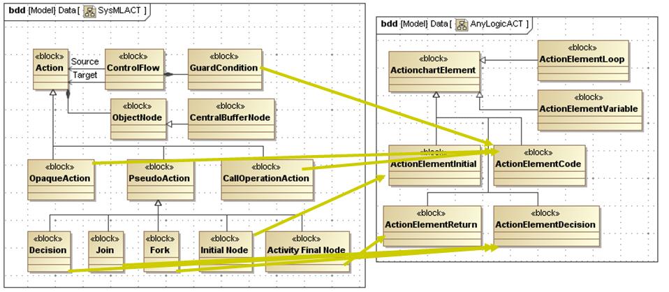
185 Figure 68: Partial mapping rules. Figure 69: Partial mapping rules. Figure 70: Partial mapping rules. 171

186 8.4.5 Transformation Procedure For any model element in the domain library denoted as m M1-SysML, the transformation procedure is specified as follows: Step 1. Identify the conforming model element m M2-SysML in the SysML meta-model. For example, if the domain library is a structural element, it may conform to a block. If it is a behavior library, it may conform to an action. Step 2. Check the mapping rules defined in section for m M2-SysML. Since the mapping rules are one-to-one or one-to-many functions, we can find the corresponding model element of the AnyLogic meta-model, denoted as m M2- AnyLogic. Step 3. Create the corresponding simulation library (m M1-AnyLogic ) in the AnyLogic which m M1-AnyLogic is a type of m M2-AnyLogic. Step 4. If m M1-SysML has any property, value or relationship, each of them also is transformed to the AnyLogic language by repeating Steps 1 to 3. We can apply this transformation procedure for the domain library as well as the system model. If the system model is created using the domain library, the system model has relationships, e.g., instanceof relationships or inheritance relationships, to the domain library. By applying the transformation procedure, the elements of the system model will be created in Steps 1 to 3 and their properties, values and relationships are transformed in Step 4. The proposed transformation procedure assumes that the mapping rules between the SysML meta-model and AnyLogic meta-model exists, i.e., each modeling element in the SysML meta-model has at least one related mapping rule. If a specific modeling element in the SysML meta-model does not have any related mapping rule, the transformation procedure will stop at Step 2. As a result, all modeling elements in the system model conforming to this SysML meta-model element will not be transformed to the simulation model. The transformation procedure is developed using Java language. The SysML model is exported as an XMI file [6] which is a type of xml file. The model data is extracted from the xmi file using Xpath [7] which enables filtering the model data to 172

187 identify the relevant SysML model elements, which are then translated to their corresponding AnyLogic implement using Java code. 8.5 Demonstration We create a SysML model of the tandem queue example. There are two parts of this example: creating the domain library and using this library to model a specific system. The domain library can be created once and used for different applications. We define the libraries of machines, buffers, arrival processes, and dispose processes. Each one includes its own parts, properties, ports and operations. Figure 71 shows a partial structure of a machine. The attribute processjob represents the entity processing in the machine. The inputport and outputport are the entry point and exit point of the machine, respectively. The operation checkcapacity will return true if the machine is occupied. The detail of this operation is captured in an activity diagram. Figure 72 shows a partial behavior of the machine as a state machine model. When processjob is empty, the machine is in the idle state. Otherwise, the machine is in the busy state. These domain libraries can be modified without changing the transformation script. This enables to reuse a domain specific language, i.e., we can create domain specific languages by extending other domain specific language without changing the transformation script. For example, we can create a new library called CuttingMachine by extending the machine library and adding new attribute speed or operation cut. Since both two libraries are described using SysML, the same transformation script can be used to transform both models into the simulation models. Figure 71: Partial structure of the machine library. 173

188 Figure 72: Partial behavior of the machine library. After defining the library, we can use it to create a specific tandem queue example and assign the attribute values such as the process time. All of the libraries and the specific systems can be exported to an XMI file and transformed into the AnyLogic project file. This generated file can be opened in AnyLogic shown in Figure 73. We show the generated machine description of the AnyLogic project file in Figure 74. If the structure and behavior are both captured in the SysML model, the generated model can be simulated. Figure 73: Generated AnyLogic project. 174