Masking Lidar Cliff-Edge Artifacts

Transcription

1 Masking Lidar Cliff-Edge Artifacts Methods 6/12/2014 Authors: Abigail Schaaf is a Remote Sensing Specialist at RedCastle Resources, Inc., working on site at the Remote Sensing Applications Center in Salt Lake City, Utah. Brent Mitchell is a Lidar Specialist and Training Group Leader at RedCastle Resources, Inc., working on site at the Remote Sensing Applications Center in Salt Lake City, Utah. Kim McCallum is a Remote Sensing Specialist at RedCastle Resources, Inc., working on site at the Remote Sensing Applications Center in Salt Lake City, Utah. Mark Beaty is a Remote Sensing Specialist at RedCastle Resources, Inc., working on site at the Remote Sensing Applications Center in Salt Lake City, Utah. Pete Joria is a Remote Sensing Specialist with the USFS R3 Regional Office. Tom Mellin is the Remote Sensing Coordinator for the USFS R3. 1

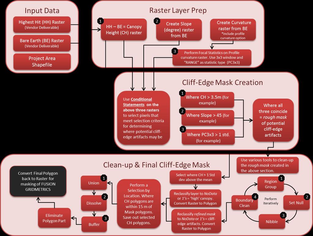
2 Introduction The primary purpose of this document is to illustrate and describe how to identify areas of false vegetation heights that appear in lidar derivatives along areas of extreme relief, such as cliff edges. Lidar vegetation heights in these cliff-edge areas contain falsely high values due to how the lidar points are processed and classified by the vendor when creating the bare earth (BE) surface (figure 1). These errors can be easily visualized in a canopy height (CH) surface, which is created by subtracting the bare earth surface from the highest hit surface both of which are typically delivered by the vendor. In the canopy height surface the errors appear as long, linear features with high height values that follow topographic contours. The false canopy height values are propagated into all the height and canopy density statistics that are generated across the landscape to describe the forest canopy structure, hence it is wise to mask them out for further analysis. These cliff-edge artifacts are displayed in red in figure 2, where the difference between the highest hit layer and the underlying bare earth surface are relatively large. Unfortunately, difference values associated with cliff-edge errors are difficult to distinguish from actual vegetation heights. High height values associated with trees are visible in the canopy height (A) image in figure 2 as the relatively small circular red and yellow areas and are similar in actual value to the cliff-edge artifact heights. This document presents a process for identifying areas where these cliff-edge artifacts are most likely to occur (figure 1) in order to generate a mask to exclude these areas from future analyses of the forest canopy structure. A Figure 1. Image A shows all points classified by the vendor as bare earth these points are used to create the bare earth surface. Image B shows bare earth points as pink, and all other points in blue. All the blue points will go into creating the highest hit surface and other vegetation structure metrics. NOTE: the blue points on the side of the cliff face are the cause of the false vegetation and cliff-edge artifacts explored in this document. B 2

3 3

4 Overview of Methods RSAC has developed a process using Esri s ArcMap software and tools to identify cliff-edge artifacts using vendor delivered products such as the highest-hit (HH) surface and the bare earth (BE) surface. The process is outlined below as an overview of the major steps involved, including important parameter settings and other pertinent considerations. Assumptions: - The user has ArcMap 10.x installed and licensed - The user has basic GIS skills which are necessary to successfully implement the process described - The user has a basic understanding of lidar-derived metrics and geoprocessing in ArcMap - The user has the Spatial Analyst extension licensed and activated KEY STEP: 1. Create a File Geodatabase (Catalog > File Directory of your choice > right-click > New > File Geodatabase > Cliff_edge.gdb). This serves two purposes 1) provides a place to keep track of all your files (primary, intermediate, and final), and 2) will force the raster outputs from each step to an ESRI Grid file format which is important for the process to work correctly as it is outlined below. Create Primary Rasters In this first section you will create the primary rasters (figure 2) for processing. You will use the BE surface and Canopy Height (CH) layer, which is created by subtracting the BE from the HH layer, to focus in on cliff areas with potential vegetation height artifacts. 2. Mosaic together the highest-hit (HH) and bare earth (BE) surfaces (source rasters) provided by the vendor. A. Use the Mosaic To New Raster tool (Data Management > Raster > Raster Dataset) to create a seamless output for each source raster (make sure you have created your File Geodatabase!). 3. Generate the primary rasters from the source rasters (HH and BE). B. Canopy Height Subtract the BE from the HH (i.e. HH BE) using the Raster Calculator (Spatial Analyst > Map Algebra). C. Slope Use the Slope tool under the Spatial Analyst > Surface toolbox and create the slope in degrees. D. Profile Curvature Use the Curvature tool under the Spatial Analyst > Surface toolbox and create both the Curvature and Profile curve raster. The latter is indicated as an optional step in the tool, seen in the graphic to the right as Output profile curve raster, however, make sure you set the output location and name to ensure this layer gets created. The profile curvature is the second derivative of 4

5 the slope ( the slope of the slope ), and captures the areas where the slope changes most quickly, for example at cliff faces. E. Profile Curvature 3x3 - Use the Focal Statistics tool (Spatial Analyst > Neighborhood) to perform a focal analysis on the Profile Curvature raster. This will enhance the cliff edge areas in hopes of creating a more inclusive and less noisy cliff-edge mask. Change the Statistic type from the drop down menu to RANGE and leave the defaults for all the other parameters. A B C Figure 2. The three primary rasters: canopy height (A), slope (B), and profile curvature 3x3 (C). NOTE: The DEM derived layers (slope and curvature) do not fully capture the cliff-edge artifacts compare the fuller red artifact area of the canopy height layer (white arrow) to the artifact areas in the other two layers (black arrows). Cliff-edge Identification/Mask Creation In this section you will perform some threshold operations on the primary rasters to determine areas where there is a very high likelihood of cliff-edge artifacts. The idea is to be more inclusive than exclusive. Remember you are mapping cliff areas and will probably not be interested in actively managing the vegetation in these areas, so inclusion of small vegetated areas in your mask will have minimal impact. Areas where all three criteria of the secondary rasters (that you will create below) coincide are considered potential cliff-edge artifacts. 4. Use the 3 primary rasters (created above) and define thresholds to create secondary products to use in identifying the cliff-edge locations. For the following processes use the Con tool under the Spatial Analyst -> Conditional toolbox (unless noted otherwise). A. First you want to select only those vegetation heights that are over a certain value. If value of canopy height raster > 3.5 meters, then re-class value = 1, else re-class value = 0 (see graphic). i. Input raster = canopy height raster 5

6 ii. Expression = Value >3.5 iii. Input true value = 1 iv. Input false value = 0 NOTE: it is probably a good idea to use the same minimum vegetation height condition (e.g., 3.5 meters in this example) as you used for the height cutoff value when generating height statistics using the LTK Processor in FUSION. This ensures that only those areas with lidar returns that were high enough to affect the GRIDMETRICS outputs will be considered for masking. For more details on GRIDMETRICS and generating canopy structure statistics please refer to the Large Lidar Acquisition Processing Workflow Tutorial: ( B. Next you will select areas that are considered steep slopes. To do this, use the Con tool. i. Input raster = slope raster ii. Expression = Value > 45, iii. Input true value = 1 iv. Input false value = 0 C. Next, you will capture local areas where the slope changes abruptly, such as cliff edges, using the profile curvature 3x3 raster (from Step E). i. Input raster = profile curvature 3x3 ii. Expression = Value > 1 standard deviation above mean iii. Input true value = 1 iv. Input false value = 0 NOTE: You will need to add the mean and the standard deviation values together to determine the value to input in the conditional. You can find the appropriate standard deviation and mean values under Layer properties > Source Tab > scroll down to the Statistics section (see outlined area in graphic to right). 5. Create a rough artifact mask using Raster Calculator by multiplying together all three of the secondary rasters (created in the steps above). Areas where the product equals 1 are identified as potential cliffedge artifact areas. All other areas are coded to zero. 6

7 Mask Clean Up In this section you will take the rough artifact mask created from the previous section and perform some clean up on it (similar to a clump and sieve process) to refine the mask. The rough artifact mask (yellow areas in the graphic at right) contains many small groups of pixels that were created during the above processing and that will cause problems when trying to apply the mask to a coarser resolution dataset (i.e., the 25m GRIDMETRICS). Your result after the clean up would be similar to the graphic below with the red cliffedge areas. In both graphics, the cliff-edge artifact values should be 1 and the non-cliff edges should be Refine the rough artifact mask through a smoothing process, using the Spatial Analyst toolbox. A. Input the rough artifact mask created in Step 5 into the Region Group tool (Spatial Analyst > Generalization). i. Use EIGHT neighbors and keep the Zone Grouping Method to WITHIN. This identifies individual clumps, or contiguous areas, of potential artifacts. This process will identify each group of contiguous pixels in the rough artifact mask that share the same value (either zero or 1), then assign a sequential number to each of these groups in the output raster. B. Use the Set Null tool (Spatial Analyst -> Conditional) with the result from Step 6.A as the input. This step creates the sieve that eliminates, or sets to NoData, all clumps that are smaller than the specified number of pixels. The output will consist only of 1 s where there are clumps of pixels greater than the set size, and NoData where there are clumps smaller than the set size. Determining the size of clumps to get rid of may take some trial and error (this is how we came up with the number 41 below) here you are trying to eliminate the tree crowns that are being incorrectly included in the mask. i. Enter the expression Count < 41 into the Expression field. (this will set all those clumps of pixels that meet this criteria to NoData) ii. Enter the number 1 into the Input false raster or constant value field (see graphic above). C. Use the Nibble tool (Spatial Analyst > Generalization) and the output from the Set Null function. Pixels that had a value of 1 will be assigned the pixel value from that same location in the raster 7

8 Rough Artifact Mask; NoData pixels will be assigned either a 1 or a zero (based on the closest non-nodata pixel from the Step 6B output and the corresponding value for that pixel location from the Rough Artifact Mask). i. Input raster = Rough Artifact Mask from Step 5. ii. Input raster mask = the output from Step 6.B (SetNull raster where NoData = clumps less than desired size). Note: The output from this process is a raster where 1 s = the cliff-edge artifact areas and 0 s equal everything else. D. Lastly, use the Boundary Clean tool using the output from Step 6.C. i. Input = output from previous step ii. Sorting technique = ASCEND * (optionally uncheck the Run expansion and shrinking twice if your results are getting rid of too many pixels or shrinking groups of pixels down to a single pixel). This is your Refined Artifact mask. This step should expand the boundary between segments to create a more continuous mask. E. If the mask needs to be refined further (based on visual inspection in ArcMap), repeat steps A-D, using the output from Step D (Refined Artifact mask) wherever the Rough Artifact mask was used previously. 7. Use the Reclassify tool (Spatial Analyst -> Reclass) on the cleaned up mask to reclass the 0 values to NoData. A. Select the final cleaned up raster from Step E as your input raster, and make sure the column New Values looks like the graphic to the right (0 becomes NoData and 1 stays as 1). This will reclassify your data, creating an output where 1 = cliffedge artifacts and NoData = rest of the area. 8. Use the Raster to Polygon tool (Conversion -> From Raster) to convert the output from Step 7. A. Uncheck Simplify polygons. Proximity analysis In this section you will use the final refined mask from the section above and the original canopy height raster to locate artifact areas near the cliff-edges that were not picked up by the previous processing steps. In rare 8

9 occasions some artifacts are missed as a result of severe misclassification of the bare earth points used to create the bare earth (BE) surface (see figure 1). In other words, when the BE surface is created by the vendor, points on overhanging cliffs do not always get classified as bare earth, and therefore these cliff areas underneath the overhang are flat in the DEM and the overhanging cliff face creates artifacts. When thresholds are set on the primary slope raster for secondary raster creation, these areas are missed because they are not greater than 45 degrees in slope. This means during the multiplication of the three secondary rasters, the areas where the DEM is wrong are missed and not included in the remaining masking process. The result of this misclassification is height artifacts which are clearly visible in the canopy height layer (see figure 3). Therefore you will use the vegetation heights to identify potential artifacts by evaluating those selected heights within a proximity to the cliff-edges already determined. 9. First you will need to take the original canopy height raster and determine the mean and standard deviation (from the Layer Properties). Add the two together and use the Conditional tool to select those canopy height values that are greater than 1 standard deviation above the mean. 10. Next, use the Reclassify tool to (Spatial Analyst -> Reclass) to reclass the 0 values to NoData and keep the 1 values as Then, convert the reclassified canopy height raster to polygon. Use the Raster to Polygon tool (Conversion -> From Raster) to convert the canopy height raster. A. Uncheck Simplify polygons. 12. Use the Select By Location tool from the Selection Menu on the main toolbar to select canopy height polygons (created in Step 11) that are within 15 meters of the mask features. You will have to use some trial and error to determine the best distance value to use here. If you make this distance too large you risk the chance of including trees in the mask that shouldn t be included, and if you make it too small you may miss other artifacts that should be included. A. Set the canopy height polygon as the select features from. B. Set the Source Layer to the polygon version of the refined mask layer from Step 8. C. Set the Selection method to are within a distance of the source layer feature D. Set the distance to 15 and the units to Meters. 13. Save the selected features using the Date -> Export Data option found in the menu when you right-click the canopy height polygon in the Table of Contents. A. Make sure the Export: Selected features option is set. 14. Use the Union tool from the Geoprocessing menu on the main toolbar to union together the output from Step 11 with the refined mask polygon layer (Step 8). 15. Use the Dissolve tool from the Geoprocessing menu on the main toolbar to dissolve the main new small polygons created from the Union into larger aggregate features. Use output from Step 14 as input. 9

10 A Figure 3. The results of three different buffer sizes applied to the canopy height layer (warm colors are taller vegetation and cooler colors are shorter vegetation). Image A shows 5m buffer applied, Image B shows 10m buffer applied, and Image C shows 15m buffer applied. B C 16. Use the Buffer tool from the Geoprocessing menu on the main toolbar to buffer the polygons by 15 meters (or more depending on your data we found that using a distance at least ½ the width of the pixel size of the lidar metrics being masked was necessary. In our case the canopy structure rasters were all at a resolution of 20 meters, so we choose 15m to ensure all artifacts were masked. Remember this is a model and no models are perfect but some are acceptable; you might want to experiment with different buffer sizes). See figure 3 for examples of different buffer sizes. Use output from Step 14 as input. 17. Use the Eliminate Polygon Part tool (Data Management -> Generalization) to eliminate interior donut holes caused by the above 3 processes. Use output from Step 16 as input. A. Set the Condition to Percent. B. Set the Percentage to 1 (this will ensure we clean out the noise but do not make major changes to the mask). The tool will eliminate parts of the feature class that are smaller than the set percentage of the features total area. Since our polygon is very large, 1 percent should be appropriate for removing the small islands in the masking areas. Final Extraction Mask 18. Use the output from Step 17 and the Erase tool (Analysis Tools > Overlay) to remove the cliff-edge features from the Study Area polygon. 19. Use the Polygon to Raster tool (Conversion Tools > To Raster) to convert your study area with cliff-edge artifacts now masked out into an area of interest in raster form. Converting it to a raster will speed up the processing time when applying the mask to your lidar metrics. A. Set your input feature as the output from Step 18. B. Make sure to set the Cellsize to 1. This will ensure you keep the detailed nature of the features when you convert it to a raster. 10

11 C. Leave all other defaults. D. Name your output > this is the FINAL mask! 20. Lastly, apply the final mask of interest to the lidar metrics to extract those parts of the raster that you want to keep and excluding those areas that have been identified as cliff-edge artifact areas. Use the Con tool (Spatial Analyst > Conditional) E. Input raster = Final Raster Mask (from Step D above) F. Expression = Value = 0 G. Input true = a lidar metric of your choosing (e.g. elev_p95_2plus_25meters) H. IMPORTANT: click the Environments button and set the Processing Extent > Snap Raster to that of your input lidar metric raster. This will ensure your masked output will align (not be shifted) with the unmasked input of the same metric. I. See final output - Figure 4. A Figure 4. Canopy height layer before and after masking out the cliff-edge artifacts (seen as long, linear red features in Image A) using the 10 m buffer. Warmer colors indicate taller vegetation and cooler colors indicate shorter vegetation. 11 B