A Maple Package for Solving and Displaying

Transcription

1 Classroom Tips and Techniques: A Package for Graphing Solution Sets of Nonlinear Inequalities Introduction Robert J. Lopez Emeritus Professor of Mathematics and Maple Fellow Maplesoft, a division of Waterloo Maple Inc., 2006 Maple's inequal command in the plots package will graph the feasible region for a set of linear inequalities. Even though Maple's solve command can solve some nonlinear inequalities exactly, Maple does not have specific tools for graphing solution sets of nonlinear inequalities. As we show in Example 6, the contourplot command (or even the plot3d command) can be used to graph the feasible region for an inequality of the form Considerably more effort must be exerted to graph the points satisfying several such inequalities. And although Maple can shade the region between a curve and the horizontal axis, it cannot easily shade the region between two arbitrary curves. In October 2005 the Maple Applications Center ( acquired A Maple Package for Solving and Displaying

2 Inequalities Robert Ipanaqué Chero National University of Piura an application that addresses several of these Maple shortcomings. You may view the original application here: By example, some taken from the author's work itself, this month's column will illustrate the usercontributed InequalityGraphics package and its applicability to classroom tasks. This package provides two commands, namely, inequalityplot and complexinequalityplot. The inequalityplot command will graph the two-dimensional feasible region for a set of nonlinear inequalities in two variables, that is, inequalities of the form Consequently, by plotting the solution set of the inequalities and the region between arbitrary plane curves can be shaded. The complexinequalityplot command will plot the solution set of one or more inequalities of the form where is a real-valued function and the functions are complex-valued functions of the complex variable In essence, however, the inequality is nothing more than because of the definition of. excludedcolor = colorname feasiblecolor = colorname linespoints = positive integer feasiblepoints = positive integer thickness = positive integer color = colorname Color of the non-feasible region Color of the feasible region Number of points plotted along curves separati Number of points computed inside feasible reg Thickness of curves separating feasible and non Color of curves separating feasible and non-fea Table 1 Options for the inequalityplot and complexinequalityplot commands in the InequalityGraphics pack To make it easier for perusing the functionality of the package, a working version of the the code for the InequalityGraphics package is embedded in Initializations section, below. Too often the process of installing a third-party package is a hurdle that prevents a user from trying out the new commands. The downloaded code for the package ( contains the three files applications. hdb, applications.ind, and applications.lib. Dropping these files into the LIB folder of a Maple 10 installation will give permanent access to the package. The name "applications" can be changed to

3 something more meaningful, like InequalityGraphics, with no ill effects. The ".ind" and ".lib" files provide the mathematical functionality of the package, whereas the ".hdb" file provides help pages without which the command of the package will still function. The one help page provided by the hdb file can be accessed with the command?inequals; We leave these matters to the reader whose interest in the package is sufficiently sparked by this article. The code available from the Application Center colors the non-feasible region white, by default, whereas the code embedded in this article colors it black. Hence, in this article we have explicitly used the option excludedcolor = white. Initializations restart; with(plots): interface(warnlevel=0): InequalityGraphics := module() export inequalityplot, complexinequalityplot; option package; inequalityplot:=proc() local ineq,ineqset,xx,yy,phaseselection,phase1,phase2, phases,var1, var2,xmin,xmax,ymin,ymax,dx,dy,jumpprecision, findjump,reg,c,p,x1,y1,p1list,p2list,aux1,aux2,jump1, jump2,eq,cc,ops,fc,ec,ls,fb,fp,lp,llss; if nargs<3 then ERROR(`expecting 3 arguments, got 0. This commmand also incorporates the options: (1) exludedcolor=yellow, (2) feasiblecolor=red, (3) linespoints=350, (4) feasiblepoints=15 and (5) thickness=1. Examples: <1> inequalityplot(x^2+y^2<1,x=-1..1,y=-1..1), <2> inequalityplot(x^2+y^2<1,x=-1..1,y=-1..1, excludedcolor=white,feasiblecolor=cyan)`) fi: ineq:=`if`(whattype(args[1])=set,convert(args[1],`and`),args

4 [1]): xx:=args[2]:yy:=args[3]: if whattype(args[1])=set then ineqset:=args[1] elif whattype(ineq)=`<` or whattype(ineq)=`>` or whattype(ineq)=`<=` or whattype(ineq)=`>=` then ineqset:={ineq} else ineqset:=convert(ineq,set) fi: var1:=lhs(xx):var2:=lhs(yy): if not(depends(ineq,var1) and depends(ineq,var2)) then ERROR(ineq,`doesn't depend on`,var1,`and`,var2) fi: ops:=[args[4..nargs]]: if not hasoption(ops,feasiblecolor,fc,'ops') then fc:=color(rgb,.70,.70,1.0) fi: if not hasoption(ops,excludedcolor,ec,'ops') then ec:=color(rgb,.20,.20,.20) fi: if not hasoption(ops,feasiblepoints,fp,'ops') then fp:=15 fi: if not hasoption(ops,linespoints,lp,'ops') then lp:=350 fi: phaseselection:=unapply(piecewise(ineq,1,2),var1,var2): phase1:=(a,b)->1:phase2:=(a,b)->0:phases:=[phase1,phase2]: xmin:=lhs(rhs(xx)): xmax:=rhs(rhs(xx)): ymin:=lhs(rhs(yy)): ymax:=rhs(rhs(yy)): dx:=(xmax-xmin)/(fp-1): dy:=(ymax-ymin)/(fp-1): jumpprecision:=.02*min(dx,dy): findjump:=(l,r)-> `if`(evalm((l-r)&*(l-r))<jumpprecision^2,.5*(l+r), `if`(phaseselection(op(l))=phaseselection(op(.5*(l+r))), findjump(.5*(l+r),r),findjump(l,.5*(l+r)) )

5 ): reg:=[]: for y1 from ymin by dy while y1<=ymax-dy do for x1 from xmin by dx while x1<=xmax-dx do c(1):=[x1,y1]: c(2):=[x1+dx,y1]: c(3):=[x1+dx,y1+dy]: c(4):=[x1,y1+dy]: p(1):=phaseselection(op(c(1))): p(2):=phaseselection(op(c(2))): p(3):=phaseselection(op(c(3))): p(4):=phaseselection(op(c(4))): if p(1)=p(2) and p(2)=p(3) and p(3)=p(4) then reg:=[op(reg), POLYGONS( [seq(`if`(phases[p(1)](op(c(n)))=1,c(n),null), n=1..4)], op(convert(color=fc,plotoptions)))] else p1list:=[1]: if p(2)=p(1) then p1list:=[op(p1list),2]: if p(3)=p(1) then p1list:=[op(p1list),3] fi fi: if p(4)=p(1) then p1list:=[4,op(p1list)]: if p(3)=p(1) then p1list:=[3,op(p1list)] fi fi: p2list:=convert({1,2,3,4} minus {op(p1list)},list): jump1:=findjump(c(p1list[nops(p1list)]), c(p2list[1])): jump2:=findjump(c(p2list[nops(p2list)]), c(p1list[1])): aux1:=[jump2,op(map(c,p1list)),jump1]:

6 aux2:=[jump1,op(map(c,p2list)),jump2]: reg:=[op(reg), POLYGONS( [seq( `if`(phases[p(1)](op(aux1[i]))=1,aux1[i],null), i=1..nops(aux1))], op(convert(color=fc,plotoptions))), POLYGONS( [seq( `if`(phases[p(p2list[1])](op(aux2[i]))=1,aux2[i], NULL), i=1..nops(aux2))], op(convert(color=fc,plotoptions))) ] fi od od: ls:=(is)-> piecewise( whattype(is)=`<` or whattype(is)=`>`,2, whattype(is)=`<=` or whattype(is)=`>=`,1 ): llss:=map(ls,[op(ineqset)]): eq:= `if`(whattype(ineqset)=set, [seq(convert(ineqset[i],equality),i=1..nops(ineqset))], [convert(ineq,equality)] ): cc:=[seq(implicitplot(eq[i],xx,yy,color=black,numpoints=lp), i=1..nops(eq))]: PLOT(op(reg), seq( CURVES(op(op(cc[i])[1]),LINESTYLE(llss[i])),i=1..nops(cc) ), op(convert(ops,plotoptions)), POLYGONS([[xmin,ymin],[xmin,ymax],[xmax,ymax], [xmax,ymin],[xmin,ymin]], op(convert(color=ec,plotoptions))), SCALING(CONSTRAINED),STYLE(PATCHNOGRID)):

7 end proc; complexinequalityplot:=proc() local ineq,var,revar,imvar,ops; if nargs<2 then ERROR(`expecting 2 arguments, got 0. This commmand also incorporates the options: (1) exludedcolor=yellow, (2) feasiblecolor=red, (3) linespoints=350, (4) feasiblepoints=15, (5) linescolor=black and (6) thickness=1. Examples: <1> complexinequalityplot(abs(z)<1,z=(-1..1,-1..1) ), <2> complexinequalityplot(abs(z)<1,z=(-1..1,-1..1), excludedcolor=white,feasiblecolor=cyan)`) fi: var:=lhs(args[2]): Revar:=rhs(args[2])[1]: Imvar:=rhs(args[2])[2]: ineq:=subs(var=x+i*y,args[1]): ops:=args[3..nargs]: inequalityplot(ineq,x=revar,y=imvar,ops) end proc; end module: with(inequalitygraphics); Examples Example 0

8 When working with the Laplace transform, the convolution product of and is defined by = The convolution of the functions and (3.1.1) (3.1.2) is difficult to obtain by the definition because of the complex nature of the implied conditionals in both The integrand of the convolution integral is nonzero on the solution set of the inequalities (3.1.3) Figure 0.1, created with Maple's built-in inequal command from the plots package, displays this set in red. (This command will graph only the solution set for linear inequalities.)

9 t x Figure 0.1 In red, the solution set for { } For each fixed, the integration is over the intersection of the line and the red parallelogram in Figure 0.1. Thus, we have

10 a result extremely difficult to fathom without Figure 0.1. Example 1 A graph of the solution set of the inequality (3.2.1) drawn for the square appears in Figure y x Figure 1.1 Solution set of in yellow graphed

11 Example 2 A graph of the solution set of the inequalities and appears in Figure 2.1. (3.3.1) (3.3.2) Figure 2.1 Solution set of {, } shown in gray Example 3 A graph of the solution set of the inequalities and (3.4.1) (3.4.2) (3.4.3)

12 appears in Figure 3.1. Note that more than two inequalities are enclosed in set braces in the inequalityplot command. Figure 3.1 Solution set of shown in gray Example 4 Figure 4.1 compares the solution sets of and the first on the left, the second on the right.

13

14 Figure 4.1 In gray, the solution set of in (a) and the solution set of in (b) Example 5 The set of points that satisfy either (3.6.1) (3.6.2) is graphed in Figure 5.1.

15 Figure 5.1 Gray points satisfy either Example 6 Drawn with the inequaltyplot command, Figure 6.1 shows the solution set of the inequality where is given by (3.7.1)

16 Figure 6.1 Solution set for drawn in gray Figure 6.2, drawn with the plot3d command, shows the surface for As such, it represents that part of the surface we can identify as being above the plane. Rotating the graph so that it is viewed from a point sufficiently high on the -axis gives a sketch of the feasible region similar to Figure 6.1.

17 (a)

18 (b) Figure 6.2 Graph of in (a); same graph rotated and viewed from above in (b) Figure 6.3, drawn with Maple's contourplot command, shows the graph of the curve determined by the equation. This is the boundary inside or outside of which will be satisfied.

19 y x Figure 6.3 Curve determined by solution of the equation The filled option in Maple's contourplot command shades in a specified color range according to the lowest and highest values along contours. Figure 6.4 is a contour plot of in which the color range is from white to gray, with white being assigned to any contours on which the values of are lower than the one specified for the single contour to be drawn. This specified contour value is zero, so any contour corresponding to a higher value will be shaded gray.

20 Figure 6.4 Shaded contour plot of Black curve is the single contour Gray Example 7 To shade the region between graphs of the curves and use the inequalityplot command as shown in Figure 7.1. Note that an endpoint cannot be a symbol such as or.

21 Figure 7.1 Region between and shaded gray Example 8 Nonlinear inequalities actually arise in freshman calculus when students first meet a rigorous ( ) definition of the limit: Formal Definition of Limit The real number is said to be the limit of at if, for any the inequality holds At the heart of this definition is the inequality that we would like to solve for. For example, to show that solve the inequality

22 (3.9.1) for negative. The solution set is shown in Figure 8.1 where is allowed to be both positive and Figure 8.1 Solution set for the inequality?? shaded in gray Although Maple cannot solve the inequality?? for it can solve the equation under the assumption that The solutions, namely (3.9.2)

23 are graphed in Figure 8.2 where the colors indicate which solutions assume real values. Compare Figure 8.2 to Figure epsilon Figure 8.2 Graph of the analytic solution for As with Example 6, the outline of the feasible region can be obtained with Maple's implicitplot command; the feasible region, with contourplot, as shown in Figure 8.3.

24 (a) e d 0

25 Figure 8.3 In (a), outline of feasible region via implicitplot; in (b), feasible region via contourplot Surprisingly, the feasible region in Figure 8.1 is not symmetric. Figure 8.4 shows the feasible region for much smaller values of and suggests the region might be more symmetric closer to. In fact, it suggests that might be well approximated by a linear function.

26 e 0 d Figure 8.4 Solution set for the inequality?? for "small" values of One way to find an approximation for when is small is to solve for a series solution about. This can be done in Maple via where we removed the absolute value function and created two equivalent equations. In this case we obtained exact solutions and not the series expansions and (3.9.5)

27 This suggests a hypothesis tested in Figure 8.5 where the lines are drawn in green, is drawn in black, and is drawn in red. 0 e Figure 8.5 The lines in green, in black, and in red Alternatively, we let Maple deduce true (3.9.

28 The function (3.9.9) is continuous from the right at so that The governing inequality is a graphical solution of which is seen in Figure 8.6. Figure 8.6 Shaded gray, the feasible region for the inequality For the inequality is satisfied for any positive as Figure 8.6 suggests, and the following calculation shows.

29 (3.9.10) Example 9 Drawn with the complexinequalityplot command, the solution set for the inequality where, appears as the shaded region in Figure 9.1. Figure 9.1 Solution set for shaded in gray The substitution

30 leads to (3.10.1) (3.10.2) and hence, Figure 9.2 drawn with the inequalityplot command. Figure 9.2 Solution set for (3.10.2) shaded in gray The advantages of the complexinequalityplot command over the inequalityplot command for inequalities in the complex variable are obvious, and need no comment. Example 10

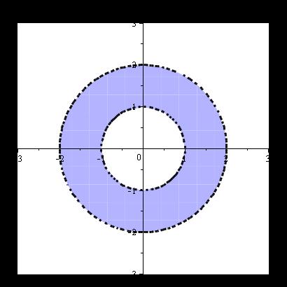
31 Like the inequalityplot command, the complexinequalityplot command will graph the feasible region for a set of nonlinear complex inequalities. For example, Figure 10.1 shows the set of points simultaneously satisfying the inequalities and (3.11.1) (3.11.2) Figure 10.1 Solution set of shaded in gray Legal Notice: The copyright for this application is owned by Maplesoft. The application is intended to demonstrate the use of Maple to solve a particular problem. It has been made available for product evaluation purposes only and may not be used in any other context without the express permission of Maplesoft.

32