PROBLEMS INVOLVING PARAMETERIZED SURFACES AND SURFACES OF REVOLUTION

Transcription

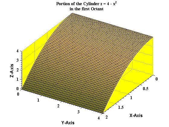
1 PROBLEMS INVOLVING PARAMETERIZED SURFACES AND SURFACES OF REVOLUTION Exercise 7.1 Plot the portion of the parabolic cylinder z = 4 - x^2 that lies in the first octant with 0 y 4. (Use parameters x and y. Determine the range of values for x to only plot points in the first octant.) clear all clc; f - x.^2; x = linspace(0,2,60); y = linspace(0,4,60); [X,Y] = meshgrid(x,y); surf(x,y,f(x,y),'facealpha',0.5) colormap copper grid on rotate3d view([154,44]) axis([ ]) set(gca,'color','y') set(gca,'xtick',0:.5:2,'xminortick','on','fontname','times','fontweight','bold') set(gca,'ytick',0:1:4,'yminortick','on','fontname','times','fontweight','bold') set(gca,'ztick',0:1:4,'zminortick','on','fontname','times','fontweight','bold') title({'portion of the Cylinder z = 4 - x^2','in the first Octant'}) xlabel('x-axis','color','black','fontname','mathematica','fontweight','bold','fontsize',12) ylabel('y-axis','color','black','fontname','mathematica','fontweight','bold','fontsize',12) zlabel('z-axis','color','black','fontname','mathematica','fontweight','bold','fontsize',12)

2

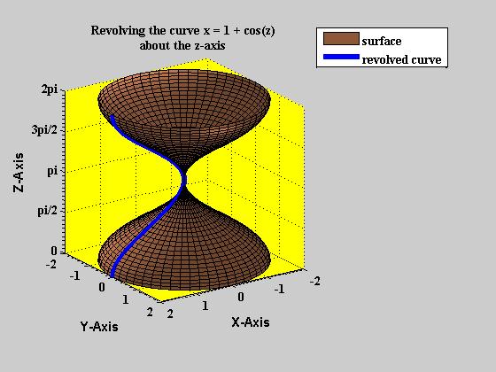
3 Exercise 7.2 Rotate the curve x = 1 + cos z, for 0 z 2π, around the z-axis. Use Matlab to draw the surface of revolution. Use axis equal command if necessary for a nondistorted view. These equations x = F(z)cos t, y = F(z) sin t, z = z rotates a function F(z) about the z-axis. Clear all clc F + cos(z); %(The funtion or curve to be rotated) t = linspace(0,2*pi,55); z = linspace(0,2*pi,55); %Rotation of the curve F(z) about the z-axis [T,U] = meshgrid(t,z); X = F(U).*cos(T); Y = F(U).*sin(T); Z = U; surfl(x,y,z); hold on % Parametrization of the curve x = 1 + cos(z) t=linspace(0,2*pi,55); x=1+cos(t); y=0.*t; z=t; plot3(x,y,z,'b','linewidth',4)

4 colormap copper grid on rotate3d view([146,20]) axis equal square axis([ *pi]) legend('surface','revolved curve','location','northeastoutside') set(gca,'color','y') set(gca,'xtick',-2:1:2,'xminortick','on','fontname','times','fontweight','bold') set(gca,'ytick',-2:1:2,'yminortick','on','fontname','times','fontweight','bold') set(gca,'ztick',0:pi/2:2*pi,'zticklabel',{'0','pi/2','pi','3pi/2','2pi'}) set(gca,'zminortick','on','fontname','times','fontweight','bold') title({'the curve x = F(z) = 1 + cos(z)','revolved about the z-axis'}) xlabel('x-axis','color','black','fontname','mathematica','fontweight','bold','fontsize',12) ylabel('y-axis','color','black','fontname','mathematica','fontweight','bold','fontsize',12) zlabel('z-axis','color','black','fontname','mathematica','fontweight','bold','fontsize',12)

5

6 Exercise 7.3 Draw the portion of the cone y^2 = x^2 + z^2 for 0 y 3. (This is obtained by rotating the line z = y around the y-axis. Use the angle of rotation t and the y variable as parameters.) clear all clc F t = linspace(0,2*pi,55); y = linspace(0,3,55); [T,Y] = meshgrid(t,y); X = F(Y).*cos(T); Z = F(Y).*sin(T); Y = Y; surfl(x,y,z); hold on X = 0.*F(y); Y = F(y); Z = F(y); plot3(x,y,z,'b','linewidth',4) colormap copper grid on rotate3d view([130,22]) axis equal square axis([ ])

7 legend('surface','revolved curve','location','northeastoutside') set(gca,'color','y','xtick',-3:1:3,'xminortick','on','fontname','times','fontweight','bold') set(gca,'ytick',0:0.5:3,'yminortick','on','fontname','times','fontweight','bold') set(gca,'ztick',-3:1:3,'zticklabel',{'0','pi/2','pi','3pi/2','2pi'}) set(gca,'zminortick','on','fontname','times','fontweight','bold') title({'revolving the curve x = 1 + cos(z)','about the z-axis'}) xlabel('x-axis','color','black','fontname','mathematica','fontweight','bold','fontsize',12) ylabel('y-axis','color','black','fontname','mathematica','fontweight','bold','fontsize',12) zlabel('z-axis','color','black','fontname','mathematica','fontweight','bold','fontsize',12)

8 Exercise 7.4 Draw the ellipsoid whose equation is x^2/4 + y^2/16 + z^2/2 = 1 in two ways. WAY 1: Using explicit parametric equations base on spherical coordinates. (Observe: The quantities x' = x/2, y' = y/4 and z' = z/sqrt(2) satisfy the equation (x')^2 + ( y')^2 + (z')^2 = 1. Use spherical coordinates for x', y', and z' to parametrize the latter surface.) Use axis equal to obtain a non-distorted view. WAY 2: Using the MatLab built-in function ellipsoid. THE CODE FOR WAY 1 u = linspace(0,pi,60); v = linspace (0,2*pi,60); [U,V] = meshgrid(u,v); X = 2*sin(U).*cos(V); Y = 4*sin(U).*sin(V); Z = sqrt(2)*cos(u); surfl(x,y,z) colormap copper grid on rotate3d axis equal axis([ sqrt(2),sqrt(2)]) view([158,14]) set(gca,'color','y','xtick',-2:1:2,'xminortick','on','fontname','times','fontweight','bold') set(gca,'ytick',-4:1:4,'yminortick','on','fontname','times','fontweight','bold') set(gca,'ztick',-2:0.5:2,'zminortick','on','fontname','times','fontweight','bold')

9 title('a Parameterized Ellipsoid 4x^2 + y^2 + 8z^2 = 16') xlabel('x-axis','color','black','fontname','mathematica','fontweight','bold','fontsize',12) ylabel('y-axis','color','black','fontname','mathematica','fontweight','bold','fontsize',12) zlabel('z-axis','color','black','fontname','mathematica','fontweight','bold','fontsize',12)

10 CODE FOR WAY 2 Clear all clc [x,y,z] = ellipsoid(0,0,0,2,4,sqrt(2),40); surfl(x,y,z) colormap copper grid on rotate3d axis equal axis([ sqrt(2),sqrt(2)]) view([158,14]) set(gca,'color','y') set(gca,'xtick',-2:1:2,'xminortick','on','fontname','times','fontweight','bold') set(gca,'ytick',-4:1:4,'yminortick','on','fontname','times','fontweight','bold') set(gca,'ztick',-2:0.5:2,'zminortick','on','fontname','times','fontweight','bold') title('an Ellipsoid 4x^2 + y^2 + 8z^2 = 16 (generated by the Ellipsoid Command)') xlabel('x-axis','color','black','fontname','mathematica','fontweight','bold','fontsize',12) ylabel('y-axis','color','black','fontname','mathematica','fontweight','bold','fontsize',12) zlabel('z-axis','color','black','fontname','mathematica','fontweight','bold','fontsize',12)

11

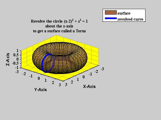
12 Exercise 7.5 The circle of radius 1 centered at (2,0,0) in the xz-plane has parametric equations x = 2 + cos t, y = 0, z = sin t, where 0 t 2π. If we revolve that circle or curve around the z-axis we obtain a donut-shaped figure called a TORUS. Letting s denote the angle of rotation about the z-axis. Show that the parametric equations of this surface are x = (2 + cos t) cos s, y = (2 + cos t) sin s, z = sin t, where 0 t 2π and 0 s 2π. Using Matlab, draw the surface. (N.B. Use axis equal to obtain a non-distorted view.) clear all clc f + cos(x); g t = linspace(0,2*pi,40); s = linspace(0,2*pi,40); [T,S] = meshgrid(t,s); %The torus X = f(t).*cos(s); Y = f(t).*sin(s); Z = g(t); surf(x,y,z,'facealpha', 0.4) hold on % The circle drawn in blue that was rotated about the z-axis X = f(t); Y = 0.*f(t); Z = z(t);

13 plot3(x,y,z,'b','linewidth',4); colormap copper grid on rotate3d view([130,22]) axis equal axis([ ]) legend('surface','revolved curve','location','northeastoutside') set(gca,'color','y','xtick',-3:1:3,'xminortick','on','fontname','times','fontweight','bold') set(gca,'ytick',-3:1:3,'yminortick','on','fontname','times','fontweight','bold') set(gca,'ztick',-1:0.5:1,'zminortick','on','fontname','times','fontweight','bold') title({ The circle (x-2)^2 + z^2 = 1','revolved about the z-axis','to get a surface called a Torus'}) xlabel('x-axis','color','black','fontname','mathematica','fontweight','bold','fontsize',12) ylabel('y-axis','color','black','fontname','mathematica','fontweight','bold','fontsize',12) zlabel('z-axis','color','black','fontname','mathematica','fontweight','bold','fontsize',12)

14

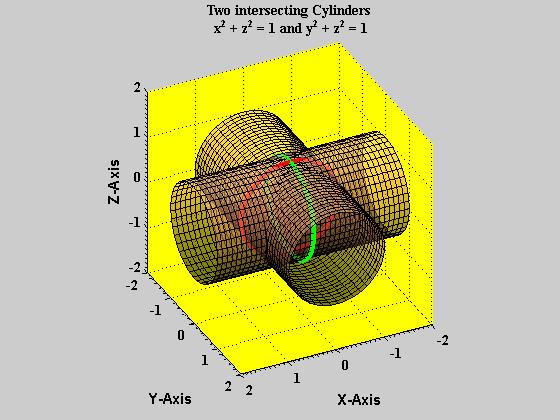
15 Exercise 7.6 Create a single plot showing the cylinders x^2 + z^2 = 1 and y^2 + z^2 = 1 within the box where -2 x 2, -2 y 2, and -2 z 2. Later we will compute the volume enclosed by the two cylinders. Make one cylinder semi-transparent using matlab s FaceAlpha property. Clear all clc x=@(w)cos(w); y=@(w)0.*w; z=@(w)sin(w); t=linspace(-2,2,40); s=linspace(0,2*pi,40); X = x(s); Y = 0.*y(s); Z = z(s); plot3(x,y,z,'r','linewidth',4) hold on X = y(s); Y = x(s); Z = z(s); plot3(x,y,z,'g','linewidth',4) [U,V] = meshgrid(t,s); X = cos(v); Y = U; Z = sin(v);

16 surf(x,y,z,'facealpha',0.5) X = U; Y = cos(v); Z = sin(v); surf(x,y,z,'facealpha',0.5) colormap copper grid on rotate3d axis equal square axis([ ]) view([154,32]) set(gca,'color','y','xtick',-2:1:2,'xminortick','on','fontname','times','fontweight','bold') set(gca,'ytick',-2:1:2,'yminortick','on','fontname','times','fontweight','bold') set(gca,'ztick',-2:1:2,'zminortick','on','fontname','times','fontweight','bold') title({'two intersecting Cylinders',' x^2 + z^2 = 1 and y^2 + z^2 = 1'}) xlabel('x-axis','color','black','fontname','mathematica','fontweight','bold','fontsize',12) ylabel('y-axis','color','black','fontname','mathematica','fontweight','bold','fontsize',12) zlabel('z-axis','color','black','fontname','mathematica','fontweight','bold','fontsize',12)

17

18 Exercise 7.7 Create a single plot showing the portion of the parabolic cylinder z = 4 - x^2 that lies in the first octant with 0 y 3, (see Exercise 7.1) and the first octant portion of the vertical plane y = x, with 0 z 4. Draw the plane with a single patch using a 'FaceColor' of 'cyan'. Make the cylinder semi-transparent so you can see the vertical plane inside the cylinder. clear all clc f - x.^2; g + 0.*z; x = linspace(0,2,60); z = linspace(0,4,60); y = linspace(0,3,60); [X,Y] = meshgrid(x,z); [X,Z] = meshgrid(x,z); surf(x,y,f(x,y),'facealpha',0.5) hold on surfl(x,g(x,z),z) colormap copper grid on rotate3d view([154,44]) axis([ ]) set(gca,'color','y','xtick',0:.5:2,'xminortick','on','fontname','times','fontweight','bold') set(gca,'ytick',0:1:4,'yminortick','on','fontname','times','fontweight','bold') set(gca,'ztick',0:1:4,'zminortick','on','fontname','times','fontweight','bold')

19 title({'portion of the Cylinder z = 4 - x^2 and vertical plane y = x','in the first Octant'}) xlabel('x-axis','color','black','fontname','mathematica','fontweight','bold','fontsize',12) ylabel('y-axis','color','black','fontname','mathematica','fontweight','bold','fontsize',12) zlabel('z-axis','color','black','fontname','mathematica','fontweight','bold','fontsize',12)

20 Exercise 7.8 Create a single plot that shows the sphere x^2 + y^2 + z^2 = 4 and the cylinder (x - 1)^2 + y^2 = 1. Use axis equal to obtain a non-distorted view. Make the sphere semitransparent so you can see the cylinder inside of it. clear all clc t = linspace(-2,2,40); u = linspace(0,pi,40); s = linspace(0,2*pi,40); [U,V] = meshgrid(u,s); %The Sphere of radius 2 centered at the origin (0,0,0. X = 2.* sin(u).* cos(v); Y = 2.* sin(u).* sin(v); Z = 2.* cos(u); surf(x,y,z,'facealpha',0.4) hold on [U,V] = meshgrid(t,s); % The cylinder at centered at (1,0,0) X = 1 + cos(v); Y = sin(v); Z = U; surf(x,y,z)

21 colormap copper grid on rotate3d view([154,44]) axis equal square axis([ ]) set(gca,'color','y','xtick',-2:1:2,'xminortick','on','fontname','times','fontweight','bold') set(gca,'ytick',-2:1:2,'yminortick','on','fontname','times','fontweight','bold') set(gca,'ztick',-2:1:2,'zminortick','on','fontname','times','fontweight','bold') title({'portion of the Cylinder z = f(x,y) = 4 - x^2', 'and the vertical plane y = x in the first Octant'}) xlabel('x-axis','color','black','fontname','mathematica','fontweight','bold','fontsize',12) ylabel('y-axis','color','black','fontname','mathematica','fontweight','bold','fontsize',12) zlabel('z-axis','color','black','fontname','mathematica','fontweight','bold','fontsize',12)

22 END OF MATLAB ASSIGNMENT 7 (READ AND DO ASSIGNMENT 8 ON YOUR OWN!!!)

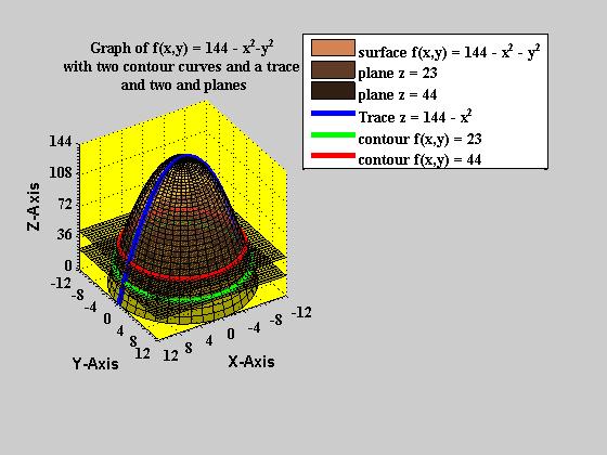
23 THIS PROBLEM (NOT A PART OF YOUR 7 TH LAB) WAS INCLUDED ONLY TO ASSIST YOU IN SOLVING PROBLEM 2 OF YOUR TAKE HOME Exercise 7.9 Sketch the surface f(x,y) = x^2 - y^2 together with these two contour curves f(x,y) = 44 and f(x,y) = 23. Include the planes z = 23 and z = 44 and the trace curve y = 0 as part of your plot. This should help you. Clear all clc % THE SURFACES TO BE PLOTTED g - x.^2; % The trace curve y = 0 This is a curve in the xz-plane. F - 0.*y; % The plane z = 44 G - 0.*y; % The plane z = 23 x = linspace(-12,12, 40); y = linspace(-12,12, 40); u = linspace(0,12,40); v = linspace(0,2*pi,40); % Parametrization of the Circular Paraboloid z = 144 x^2 y^2. [U,V] = meshgrid(u,v); % Parameter domain X = U.*cos(V); Y = U.*sin(V); Z = 144-U.^2;

24 surf(x,y,z,'facealpha',0.4) hold on [X,Y] = meshgrid(x,y); % Rectangular Domain over which I am plotting f(x,y) only surf(x,y,f(x,y),'facealpha',0.3) surf(x,y,g(x,y),'facealpha',0.3) % READY TO DEFINE PLANES z = d - ax - by. Therefore we have z = 44-0x - 0y and z = 23-0x - 0y t = linspace(-12,12,40); % Domain of the trace curve % Define the trace curve y = 0 and z = x^2 X = t; Y = 0.*t; Z = t.^2; plot3(x,y,z,'b','linewidth', 3) % Now we define the two 'Contour curves' (not level curves) f(x,y) = 44 i.e the x^2 + y^2 = 100; z = 44 and % f(x,y) = 23 i.e., x^2 + y^2 = 121; z = 23. Since these curves in space % are circles we can parameterize them in the usual way. t = linspace(0,2*pi,40); u = linspace(1,1,40); X = 11.*cos(t); Y = 11.*sin(t); Z = 23.*u;

25 plot3(x,y,z,'g','linewidth',3) X = 10.*cos(t); Y = 10.*sin(t); Z = 44.*u; plot3(x,y,z,'r','linewidth',3) colormap copper grid on rotate3d view([148,34]) axis equal square axis([ ]) legend('surface f(x,y) = x^2 - y^2','plane z = 23','plane z = 44','Trace z = x^2','contour f(x,y) = 23','contour f(x,y) = 44','Location','NorthEastOutside') set(gca,'color','y','xtick',-12:4:12,'xminortick','on','fontname','times','fontweight','bold') set(gca,'ytick',-12:4:12,'yminortick','on','fontname','times','fontweight','bold') set(gca,'ztick',0:36:144,'zminortick','on','fontname','times','fontweight','bold') title({'graph of f(x,y) = x^2-y^2','with two contour curves and a trace',' and two and planes'}) xlabel('x-axis','color','black','fontname','mathematica','fontweight','bold','fontsize',12) ylabel('y-axis','color','black','fontname','mathematica','fontweight','bold','fontsize',12) zlabel('z-axis','color','black','fontname','mathematica','fontweight','bold','fontsize',12)

26