Operations Research. Unit-I. Course Description:

Transcription

1 Operations Research Course Description: Operations Research is a very important area of study, which tracks its roots to business applications. It combines the three broad disciplines of Mathematics, Computer Science, and Business Applications. This course will formally develop the ideas of developing, analyzing, and validating mathematical models for decision problems, and their systematic solution. The course will involve programming and mathematical analysis. Course Objectives: Upon completion of this course, the students will be able to: - Solve business problems and apply it's applications by using computer programming and mathematical analysis. - Develop the ideas of developing, analyzing, and validating mathematical models for decision problems, and their systematic solution. - Understand the main concepts of OR. Unit-I Introduction The term operations research was first coined in 1940 by McClosky and Trefthen in a small town Bowdsey, of the United Kingdom. This new science came into existence in a military context. During World War II, military management called on scientists from various disciplines and organized them into teams to assist in solving strategic and tactical problems, relating to air and land defense of the country. Their mission was to formulate specific proposals and plans for aiding the Military commands to arrive at decisions on optimal utilization of scarce military resources and efforts and also to implement the decisions effectively. This new approach to the systematic and scientific study of the operations of the system was called Operations Research or operational research. Hence OR can be associated with "an art of winning the war without actually fighting it." Scope of Operations Research There is a great scope for economists, statisticians, administrators and the technicians working as a team to solve problems of defence by using the OR approach. Besides this, OR is useful in the various other important fields like: 1. Agriculture. 2. Finance. 3. Industry. 4. Marketing. 5. Personnel Management. 6. Production Management. 7. Research and Development.

2 Phases of Operational Research The procedure to be followed in the study of OR, generally involves the following major phases. 1. Formulating the problem. 2. Constructing a mathematical model. 3. Deriving the solution from the model. 4. Testing the model and its solution (updating the model). 5. Controlling the solution. 6. Implementation. Models in Operations Research A model in OR is a simplified representation of an operation, or is a process in which only the basic aspects or the most important features of a typical problem under investigation are considered. The objective of a model is to identify significant factors and interrelationships. The reliability of the solution obtained from a model, depends on the validity of the model representing the real system. A good model must possess the following characteristics: (i) It should be capable of taking into account, new formulation without having any changes in its frame. (ii) Assumptions made in the model should be as small as possible. (iii) Variables used in the model must be less in number ensuring that it is simple and coherent. (iv) It should be open to parametric type of treatment. (v) It should not take much time in its construction for any problem. Advantages of a Model There are certain significant advantages gained when using a model these are: (i) Problems under consideration become controllable through a model. (ii) It provides a logical and systematic approach to the problem. (iii) It provides the limitations and scope of an activity. (iv) It helps in finding useful tools that eliminate duplication of methods applied to solve problems. (v) It helps in finding solutions for research and improvements in a system. (vi) It provides an economic description and explanation of either the operation, or the systems they represent. Models by Structure Mathematical models are most abstract in nature. They employ a set of mathematical symbols to represent the components of the real system. These variables are related together by means of mathematical equations to describe the behavior of the system. The solution of the problem is then obtained by applying well-developed mathematical techniques to the model. BASIC OR CONCEPTS "OR is the representation of real-world systems by mathematical models together with the use of quantitative methods (algorithms) for solving such models, with a view to optimizing." We can also define a mathematical model as consisting of:

3 Decision variables, which are the unknowns to be determined by the solution to the model. Constraints to represent the physical limitations of the system An objective function An optimal solution to the model is the identification of a set of variable values which are feasible (satisfy all the constraints) and which lead to the optimal value of the objective function. An optimization model seeks to find values of the decision variables that optimize (maximize or minimize) an objective function among the set of all values for the decision variables that satisfy the given constraints. TERMINOLOGY Solution: The set of values of decision variables (j = 1, 2,... n) which satisfy the constraints is said to constitute solution to meet problem. Feasible Solution: The set of values of decision variables Xj (j = 1, 2,... n) which satisfy all the constraints and non-negativity conditions of an linear programming problem simultaneously is said to constitute the feasible solution to that problem. Infeasible Solution: The set of values of decision variables Xj (j = 1, 2,... n) which do not satisfy all the constraints and non-negativity conditions of the problem is said to constitute the infeasible solution to that linear programming problem. Basic Solution: For a set of m simultaneous equations in n variables (n > m), a solution obtained by setting (n m) variables equal to zero and solving for remaining m variables is called a basic feasible solution. The variables which are set to zero are known as non-basic variables and the remaining m variables which appear in this solution are known as basic variables: Basic Feasible Solution: A feasible solution to LP problem which is also the basic solution is called the basic feasible solution. Basic feasible solutions are of two types; (a) Degenerate: A basic feasible solution is called degenerate if value of at least one basic variable is zero. (b) Non-degenerate: A basic feasible solution is called non-degenerate if all values of m basic variables are non-zero and positive. Optimum Basic Feasible Solution: A basic feasible solution which optimizes (maximizes or minimizes) the objective function value of the given LP problem is called an optimum basic feasible solution. Unbounded Solution: A basic feasible solution which optimizes the objective function of the LP problem indefinitely is called unbounded solution. Introduction of Linear Programming Linear programming deals with the optimization (maximization or minimization) of a function of variables known as objective functions. It is subject to a set of linear equalities and /or inequalities known as constraints. Linear programming is a mathematical technique, which involves the allocation of limited resources in an optimal manner, on the basis of a given criterion of optimality.

4 In this section properties of Linear Programming Problems (LPP) are discussed. The graphical method of solving a LPP is applicable where two variables are involved. The most widely used method for solving LP problems consisting of any number of variables is called Simplex method Formulation of LP Problems The procedure for mathematical formulation of a LPP consists of the following steps: Step 1 To write down the decision variables of the problem. Step 2 To formulate the objective function to be optimized (Maximized or Minimized) as a linear function of the decision variables. Step 3 To formulate the other conditions of the problem such as resource limitation, market constraints, interrelations between variables etc., as linear in equations or equations in terms of the decision variables. Step 4 To add the non-negativity constraint from the considerations so that the negative values of the decision variables do not have any valid physical interpretation. The objective function, the set of constraint and the non-negative constraint together form a Linear programming problem. General Formulation of LPP The general formulation of the LPP can, be stated as follows: In order to find the values of n decision variables x1, x2, x3,..., xn to maximize or minimize the objective function. Z = c1x1 + c2 x cn x n (1) and also satisfy m-constraints a 11 x 1 +a 12 x 2 +.a 1n x n = b 1 a 21 x 1 +a 22 x 2 +.a 2n x n = b 2. a m1 x 1 +a m2 x 2 +.a mn x n = b m where constraints may be in the form of inequality < or > or even in the form an equation (=) and finally satisfy the nonnegative restrictions x 1, x 2, x 3,...x n 0. Ex: A manufacturer produces two types of models M1 and M2. Each model of the type M1 requires 4 hrs of grinding and 2 hours of polishing; whereas each model of the type M2 requires 2 hours of grinding and 5 hours of polishing. The manufacturers have 2 grinders and 3 polishers. Each grinder works 40 hours a week and each polisher works for 60 hours a week. Profit on M1 model is Rs.3.00 and on model M2, is Rs Whatever is produced in a week is sold in the market. How should the manufacturer allocate his production capacity to the two types of models, so that he may make the maximum profit in a week? Solution: Decision Variables: Let x 1 and x 2 be the number of units of M1 and M2 model.

5 Objective function: Since the profit on both the models are given, we have to maximize the profit Max (Z) = 3x x 2 Constraints: There are two constraints one for grinding and the other for polishing. No.of hrs. Available on each grinder for one week is 40 hrs. There are 2 grinders. Hence the manufacturer does not have more than 2 * 40 = 80 hrs of grinding. M1 requires 4 firs of grinding and M 2, requires 2 hours of grinding. The grinding constraint is given by 4x 1 + 2x 2 80 Since there are 3 polishers, the available time for polishing in a week is given by 3 x 60= 180. M1 requires 2 hrs of polishing and M2, requires 5 hrs of polishing. Hence, we have 2x 1 + 5x Finally we have Max (Z) = 3x x 2 Subject to 4x 1 + 2x x 1 + 5x GRAPHICAL METHOD: If there are two variables in an LP problem, it can be solved by graphical method. Let the two variables be x 1 and x 2. The variable x 1 is represented on x-axis and x 2 on y-axis. Due to nonnegativity condition, the variables x 1 and x 2 can assume positive values and hence the if at all solution exists for the problem, it lies in the first quadrant. The steps used in graphical method are summarized as follows: Step 1: Replace the inequality sign in each constraint by an equal to sign. Step 2: Represent the first constraint equation by a straight line on the graph. Any point on this line satisfies the first constraint equation. If the constraint inequality is _ type, then the area (region) below this line satisfies this constraint. If the constraint inequality is of _ type, then the area (region) above the line satisfies this constraint. Step 3: Repeat step 2 for all given constraints. Step 4: Shade the common portion of the graph that satisfies all the constraints simultaneously drawn so far. This shaded area is called the feasible region (or solution space) of the given LP problem. Any point inside this region is called feasible solution and provides values of x1 and x2 that satisfy all constraints. Step 5: Find the optimal solution for the given LP problem. The optimal solution may be determined using the following methods. Extreme Point Method: In this method, the coordinates of each extreme point are substituted in the objective function equation, whichever solution has optimum value of Z (maximum or minimum) is the optimal solution. Iso-Profit (Cost) Function Line Method: In this method the objective function is represented by a straight line for arbitrary value of Z. Generally the objective function line is represented by a dotted line to distinguish it from constraint lines. If the objective is to maximize the value of Z, then move the objective function line parallel till it touches the farthest extreme point. This

6 farthest extreme point gives the optimum solution. If objective is to minimize the value of Z, then move the objective function line parallel until it touches the nearest extreme point. This nearest extreme point gives the optimal solution. Ex: Solve the following LPP using graphical method. Maximize Z = 3 x1 + 4 x2 Subject to x1 + x x1 + x2 600 x1, x2 0 Solution: Represent x1, on x-axis and x2 on y-axis. Represent the constraints on x and y axis to an appropriate scale as follows: Replace the inequality sign of the first constraint by an equality sign, the first constraint becomes x1 + x2 = 450 This can be represented by a straight line x If x1 = 0, then x2 = 450 If x2 = 0, then x1 = 450 The straight line of the first constraint equation passes through coordinates (0, 450) and (450, 0) as shown in Fig. Any point lying on this line satisfies the constraint equation. Since the constraint is inequality of _ type, to satisfy this constraint inequality the solution must lie towards left of the line. Hence mark arrows at the ends of this line to indicate to which side the solution lies. Replace the inequality sign of the second constraint by an equality sign, then the constraint equation is 2 x1 + x2 = 600 This constraint equation can be represented by straight line If x1 = 0 then x2 = 600 If x2 = 0 then x1 = 300

7 The line passes through co-ordinates (0, 600) and (300,0) as shown in Fig. Any point lying on this straight line satisfies the constraint equation. Since the constraint is inequality of _ type, the solution should lie towards left of the line to satisfy this constraint inequality. The shaded area shown in figure satisfies both the constraints as well as non-negative condition. This shaded area is called the solution space or the region of feasible solutions. To Find Optimal Solution Extreme Point s Method: Name the corners or extreme points of the solution space. The solution space is OABCO. Find the coordinates of each extreme point, substitute them in objective function equation and find the value of Z as below: Extreme point C gives the maximum value of Z. Hence, the solution is x1 = 0, x2 = 450 and maximum Z = Unbounded Solution: Some of the LP problem may not have a finite solution. The values of one or more decision variables and the value of the objective function are permitted to increase infinitely without violating the feasibility condition, then the solution is said to be unbounded. It is to be noted that the solution may be unbounded for maximization type of objective function. This is because in minimization type of objective function, the lower boundary is formed by non-negative condition for decision variables. Ex: Solve the following LPP using graphical method. Max Z = 3 x x 2 Subject to x 1 x 2 1 x 1 + x x x 2 3 x 1, x 2 0 Solution: x 1 x 2 = 1 If x 1 = 0, x 2 = 1 If x 2 = 0, x 1 = 1 x 1 x 2 = 1 passes through (0, 1) (1, 0) x 1 + x 2 = 3 If x 1 = 0, x 2 = 3 If x2 = 0, x1 = 3 x 1 + x 2 = 3 passes through (0, 3) (3, 0)

8 4.5x x 2 3 If x 1 = 0, x 2 = 3 If x 2 = 0, x 2 = 2 4.5x x 2 3 passes through (0, 3) (2, 0) The solution space is in Fig. Assume Z = 6 then 6 = 3 x x 2 passes through (0, 3) (2, 0). Move the objective function line till it touches the farthest extreme point of solution space. Since there is no closing boundary for the solution space, the dotted line can be moved to infinity. That is Z will be maximum at infinite values of x1 and x2. Hence the solution is unbounded. Note: In an unbounded solution, it is not necessary that all the variables can be made arbitrarily large as Z approaches infinity. In the above problem if the second constraint is replaced by x 1 2, then, only x1 can approach infinity and x1 cannot be more than two. Infeasible Solution: Infeasibility is a condition when constraints are inconsistent (mutually exclusive) i.e., no value of the variable satisfy all of the constraints simultaneously. There is not unique (single) feasible region. It should be noted that infeasibility depends solely on constraints and has nothing to do with the objective function. Ex: Maximize Z = 3 x1 2 x2 Subject to x1 + x2 1 2 x1 + 2 x2 4 x1, x2 0 Solution: x1 + x2 = 1 passes through (0, 1) (1, 0) 2 x1 + 2 x2 = 4 passes through (0, 2) (2, 0) To satisfy the first constraint the solution must lie to the left of line AB. To satisfy the second constraint the solution must lie to the right of line CD. There is no point (x1, x2) which satisfies both the constraints simultaneously. Hence, the problem has no solution because the constraints are inconsistent.

9 Note: The geometric method of solving linear programming problems presented before. The graphical method is useful only for problems involving two decision variables and relatively few problem constraints. What happens when we need more decision variables and more problem constraints? We use an algebraic method called the simplex method, which was developed by George B. DANTZIG ( ) in 1947 while on assignment with the U.S. Department of the air force. Simplex Method Most real-world linear programming problems have more than two variables and thus are too complex for graphical solution. A procedure called the simplex method may be used to find the optimal solution to multivariable problems. The simplex method is actually an algorithm (or a set of instructions) with which we examine corner points in a methodical fashion until we arrive at the best solution- highest profit or lowest cost. Computer programs and spreadsheets are available to handle the simplex calculations for you. But you need to know what is involved behind the scenes in order to best understand their valuable outputs. Summary of the Simplex Method Add slack variables to change the constraints into equations and write all variables to the left of the equal sign and constants to the right. Write the objective function with all nonzero terms to the left of the equal sign and zero to the right. The variable to be maximized must be positive. Set up the initial simplex tableau by creating an augmented matrix from the equations, placing the equation for the objective function last. Determine a pivot element and use matrix row operations to convert the column containing the pivot element into a unit column. If negative elements still exist in the bottom row, repeat Step 4. If all elements in the bottom row are positive, the process has been completed. When the final matrix has been obtained, determine the final basic solution. This will give the maximum value for the objective function and the values of the variables where this maximum occurs. Example Maximize: P = 3x + 4y subject to:

10 x + y 4 2x + y 5 x 0, y 0 Our first step is to classify the problem. Clearly, we are going to maximize our objective function, all are variables are nonnegative, and our constraints are written with our variable combinations less than or equal to a constant. So this is a standard maximization problem and we know how to use the simplex method to solve it. We need to write our initial simplex tableau. Since we have two constraints, we need to introduce the two slack variables u and v. This gives us the equalities x + y + u = 4 2x + y +v = 5 We rewrite our objective function as 3x 4y+P = 0 and from here obtain the system of equations x + y + u = 4 2x + y = 5 3x 4y + P = 0 This gives us our initial simplex tableau: : To find the column, locate the most negative entry to the left of the vertical line (here this is 4). To find the pivot row, divide each entry in the constant column by the entry in the corresponding in the pivot column. In this case, we ll get 4/1 as the ratio for the first row and 5/1 for the ratio in the second row. The pivot row is the row corresponding to the smallest ratio, in this case 4. So our pivot element is the in the second column, first row, hence is 1. Now we perform the following row operations to get convert the pivot column to a unit column Our simplex tableau has transformed into

11 Notice that all of the entries to the left of the vertical line in the last row are nonnegative. We must stop here! To read off the solution from the table, first find the unit columns in the table. The variables above the unit columns are assigned the value in the constant column in the row where the 1 is in the unit column. Every variable above a non-unit column is set to 0. So here y = 4, v = 1, P = 16, x = 0, and u = 0. Thus, our maximum occurs when x = 0, y = 4 and the maximum value is 16. Artificial Variables Techniques INTRODUTION LPP in which constraints may also have and = signs after ensuring that all b i 0 are considered in this section. In such cases basis of matrix cannot be obtained as an identity matrix in the starting simplex table, therefore we introduce a new type of variable called the artificial variable. These variables are fictitious and cannot have any physical meaning. The artificial variable technique is a device to get the starting basic feasible solution, so that simplex procedure may be adopted as usual until the optimal solution is obtained. To solve such LPP there are two methods. (i) The Big M Method or Method of Penalties. (ii) The Two-phase Simplex Method. THE BIG M METHOD The following steps are involved in solving an LPP using the Big M method. Step 1 Express the problem in the standard form. Step 2 Add non-negative artificial variables to the left side of each of the equations corresponding to constraints of the type or = However, addition of these artificial variable causes violation of the corresponding constraints. Therefore, we would like to get rid of these variables and would not allow them to appear in the final solution. This is achieved by assigning a very large penalty (-M for maximization and + M for minimization) in the objective function. Step 3 Solve the modified LPP by simplex method, until anyone of the three cases may arise. BIG M METHOD CRIERION: OPTIMALITY The optimal solution to the augmented problem to the original problem if there are no artificial variables with non zero value in the optimal solution. BIG M METHOD CRIERION: NO FEASIBLE SOLUTION If any artificial variable is in the basis with nonzero value at the optimal solution of the augmented problem, then the original problem has no feasible solution. The solution satisfies the constraints but does not optimize the objective function, since it contains a very large penalty M and is called pseudo optimal solution. BIG M METHOD CRIERION: DEGENERATE SOLUTION If at least one artificial variable in the basis at zero level and the optimality condition is satisfied then the current solution is an optimal basic feasible solution (though degenerated solution). Note: While applying simplex method, whenever an artificial variable happens to leave the basis, we drop that artificial variable and omit all the entries corresponding to its column from the simplex table.

12 Ex : Use Big M method to Maximize z = 3x1 + 2x2 Subject to the constraints 2x 1 +x 2 2 3x 1 +4x 2 2 X 1, x 2 0 SOLUTION Step 1. Express the problem in standard form Slack variables s1 and s2 are add and subtracted from the left-hand sides of the constraint 1 and 2 respectively to convert them to equations. These variable s2 is called negative slack variable or surplus variable. Variable s1 represents excess of availability of 2 units on constraint 1, s2 represents excess of requirement of 12 on constraint 2. Since they represent 'free', the cost/profit coefficients associated with them in the objective function are zeros. The problem, therefore, can be written as follows Maximize Z = 3x 1 + 2x 2 +0s 1 +0s 1 2x 1 +x 2 +s 1 = 2 3x 1 +4x 2 - s 2 = 2 X 1, x 2, s 1, s 2 0 Step 2. Find initial basic feasible solution Putting x1 = x2 = 0, we get s1=2, s2 =-12 as the first basic solution but it is not feasible as s2 have negative values that do not satisfy the non-negativity restrictions. Therefore, we introduce artificial variables A1 in the second constraint, which take the form 2x 1 +x 2 +s 1 = 2 3x 1 +4x 2 - s 2 + A 1 = 2 X 1, x 2, s 1, s 2, A 1 0 Now artificial variables with values greater than zero violate the equality in constraints established in step1. Therefore, A1 should not appear in the final solution. To achieve this, they are assigned a large unit penalty (a large negative value, - M) in the objective function, which can be written as Maximize z = 3x 1 + 2x 2 + 0s 1 + 0s 2 MA 1 Subject to 2x 1 +x 2 +s 1 = 2 3x 1 +4x 2 - s 2 + A 1 = 2 X 1, x 2, s 1, s 2, A 1 0 Eliminating 1 A from the second equation, modified objective function can be written as Maximize z = (3 +3M)x 1 + (2+ 4M)x 2 + 0s 1 - M s 2-12M Let M =50 as default value, then, we have Maximize = z 153x x 2 + 0s -5s 2-600

13 Problem, now, has five variables and two constraints. Three of the variables have to be zeroised to get initial basic feasible solution to the 'artificial system'. Putting x 1 = x 2 = s 2 =0, we get The starting feasible solution is s 1 = 2, A 1 = 12 and z = Note that we are starting with a very heavy negative profit which we shall maximize during the solution. First iteration simplex tableau To improve this solution, we determine that x2 is the entering variable, because -202 is the smallest entry in the bottom row. Second iteration simplex tableau Since all Z coefficients and an artificial variable appears in the objective row at positive level, the solution of given LPP does not possess any feasible solution. THE TWO PHASE METHOD In the preceding section we observed that it was frequently necessary to add artificial variables to the constraints to obtain an initial basic feasible solution to an L.P. problem. If the problem is to be solved, the artificial variables must be driven to zero. The two-phase method is another method to handle these artificial variables. Here the L.P. problem is solved in two phases. PHASE I In this phase we find an initial basic feasible solution to the original problem. For this all artificial variables are to be driven to zero. To do this an artificial (Auxiliary) objective function (r) is created which is the sum of all the artificial variables. This new objective function is then

14 minimized, subject to the constraints of the given (original) problem, using the simplex method. At the end of phase I, two cases arise: TWO PHASE METHOD CRIERION: NO FEASIBLE SOLUTION If the minimum value of r > 0, and at least one artificial variable appears in the basis at a positive level, then the given problem has no feasible solution and the procedure terminates. TWO PHASE METHOD CRIERION: OPTIMALITY If the minimum value of r = 0, and no artificial variable appears in the basis, then a basic feasible solution to the given problem is obtained. The artificial column (s) are deleted for phase II computations. If the minimum value of r = 0 and one or more artificial variables appear in the basis at zero level, then a feasible solution to the original problem is obtained. However, we must take care of this artificial variable and see that it never becomes positive during phase II computations. Zero cost coefficient is assigned to this artificial variable and it is retained in the initial table of phase II. If this variable remains in the basis at zero level in all phase II computations, there is no problem. However, the problem arises if it becomes positive in some iteration. In such a case, a slightly different approach is adopted in selecting the outgoing variable. The lowest non-negative replacement ratio criterion is not adopted to find the outgoing variable. Artificial variable (or one of the artificial variables if there are more than one) is selected as the outgoing variable. The simplex method can then be applied as usual to obtain the optimal basic feasible solution to the given L.P. problem. PHASE II Use the optimum basic feasible solution of phase I as a starting solution for the original LPP. Assign the actual costs to the variable in the objective function and a zero cost to every artificial variable in the basis at zero level. Delete the artificial variable column from the table which is eliminated from the basis in phase I. Apply simplex method to the modified simplex table obtained at the end of phase I till an optimum basic feasible is obtained or till there is an indication of unbounded solution. REMARKS 1. In phase I, the iterations are stopped as soon as the value of the new (artificial) objective function becomes zero because this is its minimum value. There is no need to continue till the optimality is reached if this value becomes zero earlier than that. 2. Note that the new objective function is always of minimization type regardless of whether the original problem is of maximization or minimization type. EX: Consider the following linear programming model and solve it using the two-phase method.

15 Phase 1 The model for phase 1 with its revised objective function is shown below. The corresponding initial table is presented in Table. objective function: Min r = A1+A 2 = 160-7x 1 14x 2-18x 3+ S 1 + S 2 subject to 4x 1 +8x 2 + 6x 3 S 1 + A 1 = 64 3x 1 +6x x 3 S 2 + A 2 = 64 X 1, X 2, X 3, S 1, S 2, A 1, A 2 0 Initial Table of Phase 1 First iteration simplex tableau Optimal simplex tableau of phase 1

16 The set of basic variables in the optimal table of phase 1 does not contain artificial variables. So, the given problem has a feasible solution. Phase 2 The only one iteration of phase 2 is shown in Table one can verify that Table gives the optimal solution. The solution in Table is optimal and feasible. The optimal results are presented below. by x1=0, x2 =3.2=6/5, x3 = 6.4 and min z=153.6 Initial Table of Phase 2 Optimal Table of Phase 2 The optimal results are presented by x 1 =0, x 2 =3.2=6/5, x3 = 6.4 and min z=153.6

17 UNIT II TRANSPORTATION PROBLEM : Introduction: The Transportation problem is one of the sub classes of L.P.Ps in which the objective is to transport various quantities of a single homogeneous commodity, that are initially stored at various origins to different destinations in such a way that the total transport cost is minimum. To Achieve this objective we must know the amount and location of available supplies and the quantities demanded, In addition, we must know that costs that result from transporting one unit of commodity from various origins to various destinations. General Transportation Problem: Let a i =quantity of commodity available at origin i b j = quantity of commodity needed at destination j c ij= cost of transporting one unit of commodity from origin i to destination j x ij= quantity transported from origin i to destination j Then the problem is determined the transportation schedule so as to minimize the total transportation cost satisfying supply and demand constraints. Mathematically, the problem may be stated as a LPP as follows. Minimize z = subject to the constraints, j=1,2, n, i=1,2, n and 0, for all I and j Existence of feasible solution: A necessary and sufficient condition for existence of a feasible solution to the general transportation problem is =0 Existence of optimum solution:

18 There always exists an optimum solution to a transportation problem Basic feasible solution: The number of basic variables of the general transportation problem at any stage of feasible solution must be m+n-1. NOTE: 1. When the total demand is equal to total supply then the transportation table is said to be balanced, otherwise unbalanced. 2. The allocated cells in the transportation table will be called occupied cells and empty cells are called non-occupied cells. The transportation table: Since the transportation problem is just a special case of general LPP. Destination supply x 11 x 12. X 1n a 1 X 21 X 22. X 1n a2 X m1 X m2 X mn am b 1 b 2 b n Demand Solution of the transportation problem The solution of a transportation problem involves the following major steps. Step 1 : Formulate the given problem as a LPP. Step 2 : Setup the given LPP in the tabular form known as a Transportation table. Step 3 : Find an initial basic feasible solution that must satisfy all the supply and demand conditions. Step 4 : Examine the solution obtained in step 3 for optimality. Step 5 : If the solution is not optimum modified the shipping schedule by including that un occupied cell whose inclusion may result in an improved solution. Step 6 : Repeat Step 3 until no further improvement is possible. We shall now discuss various methods available for finding an initial basic feasible solution and then attaining an optimum solution.

19 Finding an Initial Basic Feasible Solution: There are several methods available to obtain an initial basic feasible solution however we shall discuss here the following three methods. 1. North West Corner Method 2. Least Cost Method 3. Vogles Approximation Method North West Corner Method: Step1: Select the upper left (north-west) cell of the transportation matrix and allocate the maximum possible value to X11 which is equal to min(a1,b1). Step2: If allocation made is equal to the supply available at the first source (a1 in first row), then move vertically down to the cell (2,1). If allocation made is equal to demand of the first destination (b1 in first column), then move horizontally to the cell (1,2). If a1=b1, then allocate X11= a1 or b1 and move to cell (2,2). Step3: Continue the process until an allocation is made in the south-east corner cell of the transportation table. Example: Solve the Transportation Table to find Initial Basic Feasible Solution using North-WestCornerMethod. TotalCost=19*5+30*2+30*6+40*3+70*4+20*14 = Rs D1 D2 D3 D4 Supply S1 S2 S Demand Least Cost Method : Step1: Select the cell having lowest unit cost in the entire table and allocate the minimum of supply or demand values in that cell. Step2: Then eliminate the row or column in which supply or demand is exhausted. If both the supply and demand values are same, either of the row or column can be eliminated. In case, the smallest unit cost is not unique, then select the cell where maximum allocation can be made.

20 Step3: Repeat the process with next lowest unit cost and continue until the entire available supply at various sources and demand at various destinations is satisfied. The total transportation cost obtained by this method =8*8+10*7+20*7+40*7+70*2+40*3 =Rs.814 Here, we can see that the Least Cost Method involves a lower cost than the North-West Corner Method. Vogel's Approximation Method This method also takes costs into account in allocation. Five steps are involved in applying this heuristic: Step 1: Determine the difference between the lowest two cells in all rows and columns, including dummies. Step 2: Identify the row or column with the largest difference. Ties may be broken arbitrarily. Step 3: Allocate as much as possible to the lowest-cost cell in the row or column with the highest difference. If two or more differences are equal, allocate as much as possible to the lowest-cost cell in these rows or columns. Step 4: Stop the process if all row and column requirements are met. If not, go to the next step.

21 Step 5: Recalculate the differences between the two lowest cells remaining in all rows and columns. Any row and column with zero supply or demand should not be used in calculating further differences. Then go to Step 2. The Vogel's approximation method (VAM) usually produces an optimal or near- optimal starting solution. One study found that VAM yields an optimum solution in 80 percent of the sample problems tested. The total transportation cost obtained by this method = 8*8+19*5+20*10+10*2+40*7+60*2 = Rs.779 Here, we can see that Vogel s Approximation Method involves the lowest cost than North-West Corner Method and Least Cost Method and hence is the most preferred method of finding initial basic feasible solution. Assignment problem Assignment problem is a particular class of transportation linear programming problems Supplies and demands will be integers (often 1) Traveling salesman problem is a special type of assignment problem Objectives To structure and formulate a basic assignment problem

22 To demonstrate the formulation and solution with a numerical example To formulate and solve traveling salesman problem as an assignment problem Structure of Assignment Problem Assignment problem is a special type of transportation problem in which Number of supply and demand nodes are equal. Supply from every supply node is one. Every demand node has a demand for one. Solution is required to be all integers. Goal of an general assignment problem: Find an optimal assignment of machines (laborers) to jobs without assigning an agent more than once and ensuring that all jobs are completed The objective might be to minimize the total time to complete a set of jobs, or to maximize skill ratings, maximize the total satisfaction of the group or to minimize the cost of the assignments This is subjected to the following requirements: Each machine is assigned no more than one job. Each job is assigned to exactly one machine. Formulation of Assignment Problem Consider m laborers to whom n tasks are assigned No laborer can either sit idle or do more than one task Every pair of person and assigned work has a rating Rating may be cost, satisfaction, penalty involved or time taken to finish the job N 2 such combinations of persons and jobs assigned Optimization problem: Find such job-man combinations that optimize the sum of ratings among all. Let x ij be the decision variable The objective function is m Minimize c x ij ij i 1 j 1 Since each task is assigned to exactly one laborer and each laborer is assigned only one job, the constraints are n i 1 n j 1 n x 1 for j 1,2,... n ij x 1 for i 1,2,... m ij x ij 0 or 1 Due to the special structure of the assignment problem, the solution can be found out using a more convenient method called Hungarian method.

23 Unit III Replacement

24

25

26

27

28

29

30

31

32 Unit IV Game Theory Introduction Game theory is a formal methodology and a set of techniques to study the interaction of rational agents in strategic settings. Rational here means the standard thing in economics: maximizing over well-defined objectives; strategic means that agents care not only about their own actions, but also about the actions taken by other agents. Note that decision theory which you should have seen at least a bit of last term is the study of how an individual makes decisions in non-strategic settings; hence game theory is sometimes also referred to as multi-person decision theory. The common terminology for the field comes from its putative applications to games such as poker, chess, etc. However, the applications we are usually interested in have little directly to do with such games. In particular, these are what we call zerosum games in the sense that one player s loss is another player s gain; they are games of pure conflict. In economic applications, there is typically a mixture of conflict and cooperation motives. What is a Game? A game is a formal description of a strategic situation. Game theory Game theory is the formal study of decision-making where several players must make choices that potentially affect the interests of the other players. Elements of a Game There are three main elements of a game: The players. The strategies of each player. The consequences (payoffs) for each player for every possible profile of strategy choices of all players. Fundamental Principles of Game Theory When analyzing any game, we make the following assumptions about both players: Each player makes the best possible move. Each player knows that his or her opponent is also making the best possible move. TYPES OF GAMES 1. Two-person games and n-person games. In two person games, the players may have many possible choices open to them for each play of the game but the number of player s remains only two. Hence it is called a two person game. In case of more than two persons, the game is generally called n-person game.

33 2. Zero sum game. A zero sum game is one in which the sum of the payment to all the competitors is zero for every possible outcome of the game in a game if the sum of the points won equals the sum of the points lost. 3. Two person zero sum game A game with two players, where the gain of one player equals the loss to the other is known as a two person zero sum game. It also called rectangular form. The characteristics of such a game are. (i) Only two players participate in the game. (ii) Each player has a finite number of strategies to use. (iii) Each specific strategy results in a payoff. (iv) Total payoff to the two players at the end of each play is zero. SADDLE POINT A saddle point is a position in payoff matrix where the maximum of row minima coincides with the minimum of column maxima. The payoff at the saddle point is called the value of the game. Strategy: A Strategy is a set of best choices for a player for an entire game. Pure Strategy: A pure strategy defines a specific move or action that a player will follow in every possible attainable situation in a game. Mixed strategy: A mixed strategy is an active randomization, with given probabilities that determines the player s decision. As a special case, a mixed strategy can be the deterministic choice of one of the given pure strategies. Payoff : The payoff or outcome is the state of the game at its conclusion. In games like chess the payoff is win or loss. Payoff matrix Suppose the player A has m activities and the player B has n activities. Then a payoff matrix can be formed by adopting the following rules 1. Row designations for each matrix are the activities available to player A 2. Column designations for each matrix are the activities available to player B 3. Cell entry Vij is the payment to player A in A s payoff matrix when A chooses the activity i and B chooses the activity j. 4. With a zero-sum, two-person game, the cell entry in the player B s payoff matrix will be negative of the corresponding cell entry Vij in the player A s payoff matrix so that sum of payoff matrices for player A and player B is ultimately zero.

34 Value of the game Value of the game is the maximum guaranteed game to player A (maximizing player) if both the players uses their best strategies. It is generally denoted by V and it is unique. THE MAXIMIN-MIINMAX PRINCIPLE This principle is used for the selection of optimal strategies by two players. Consider two players A and B. A is a player who wishes to maximize his gain while player B wishes to minimize his losses. Since A would like to maximize his minimum gain, we obtain for player A, the value called maximize value and the corresponding strategy is called maximize strategy. On the other hand, since player B wishes to minimize his losses, a value called the Minimax value which is the minimum of the maximum losses is found. The corresponding strategy is called the minimax strategy. When these two are equal, the corresponding strategies are called optimal strategy and the game is said to have a saddle point. The value of the game is given by the saddle point. The selection of maximin and minimax strategies by A and B is based upon the so-called maximin minimax principle which guarantees the best of the worst results. Dominance property Sometimes it is observed that one of the pure strategies of either player is always inferior to at least one of the remaining ones. The superior strategies are said to dominate the inferior ones. In such cases of dominance, we reduce the size of the payoff matrix by deleting those strategies which are dominated by others. The general rules for dominance are: I. If all the elements of a row are less than or equal to the corresponding elements of any other row then row is dominated by the row. II. If all the elements of a column are greater than or equal to the corresponding elements of other column then column, then column is dominated by the column. III. Dominated rows and columns may be deleted to reduce the size of the pay-off matrix as the optimal strategies will remain unaffected. IV. If some linear combinations of some rows dominates row, then the row will be deleted. Similar arguments follow for column.

35 UNIT V WAITING LINES Queueing theory is the mathematical study of waiting lines, or queues. Significance: We come in contact with waiting line systems, or queuing systems, everywhere and everyday. May it be waiting in line for your morning coffee, opening up your account to see your list of new messages, or stopping at a red light in a traffic intersection, you are participating in a waitinglinesystem. As a business, waiting line systems are especially important to the operations management of the organization. Structure of waiting lines: Each specific situation will be different, but waiting line systems are essentially composed of four major elements: 1. An input of customers or items to make a customer population. This population can be finite or infinite 2. A waiting line system of customers or items 3. Workstations or operations that perform one or more activities 4. A priority rule that selects the next customer or item on which the activities perform SINGLE-SERVER WAITING LINE MODEL The easiest waiting line model involves a single-server, single-line, single-phase system. The following assumptions are made when we model this environment: 1. The customers are patient (no balking, reneging, or jockeying) and come from a population that can be considered infinite. 2. Customer arrivals are described by a Poisson distribution with a mean arrival rate of ƛ_ (lambda). This means that the time between successive customer arrivals follows an exponential distribution with an average of 1/ƛ_. 3. The customer service rate is described by a Poisson distribution with a mean service rate of µ_ (mu). This means that the service time for one customer follow an exponential distribution with an average of 1/ƛ_. 4. The waiting line priority rule used is first-come, first-served. Using these assumptions, we can calculate the operating characteristics of a waiting line system using the following formulas:

36 MULTISERVER WAITING LINE MODEL In the single-line, multi server, single-phase model, customers form a single line and are served by the first server available. The model assumes that there are s identical servers, the service time distribution for each server is exponential, and the mean service time is 1/µ. Using these assumptions, we can describe the operating characteristics with the following formulas: Distribution Of Arrivals: When describing a waiting system, we need to define the manner in which customers or the waiting units are arranged for service. Waiting line formulas generally require an arrival rate, or the number of units per period (such as an average of one every six minutes). A constant arrival distribution is periodic, with exactly the same time between successive arrivals. In productive systems, the only arrivals that truly approach a constant interval period are those subject to machine control. Much more common are variable (random) arrival distributions. In observing arrivals at a service facility, we can look at them from two viewpoints: First, we can analyze the time between successive arrivals to see if the times follow some statistical distribution. Usually

37 we assume that the time between arrivals is exponentially distributed. Second, we can set some time length (T ) and try to determine how many arrivals might enter the system within T. We typically assume that the number of arrivals per time unit is Poisson distributed. Exponential Distribution In the first case, when arrivals at a service facility occur in a purely random fashion, a plot of the inter arrival times yields an exponential distribution The probability function is f (t) = λe λt where λ is the mean number of arrivals per time period. E X H I B I T TN6. 3 Poisson Distribution In the second case, where one is interested in the number of arrivals during some time period T, the distribution obtained by finding the probability of exactly n arrivals during T. If the arrival process is random, the distribution is the Poisson, and the formula is

38 UNIT VI INVENTORY

39

40

41

42

43

44

45 Unit VII Dynamic Programming: Many decision making problems involve a process that takes place in several stages in such a way that at each stage, the process is dependent on the strategy chosen. Such types of problems are called Dynamic Programming Problems. Thus dynamic programming is concerned with the theory of multi stage decision process. Principle of Optimality It may be interesting to note that the concept of dynamic programming is largely based upon the principle of optimality due to Bellman, viz., An optimal policy has the property that whatever the initial state and initial decision are, the remaining decisions must continue an optimal policy with regard to the state resulting from the first decision The principle of optimality implies that given the initial state of a system, an optimal policy for the subsequent stage does not depend upon the policy adopted at the preceding stages. That is, the effect of a current policy decision on any of the policy decisions of the preceding stages need not be taken into account at all. It is usually referred to as the Markovian property of dynamic programming.

46

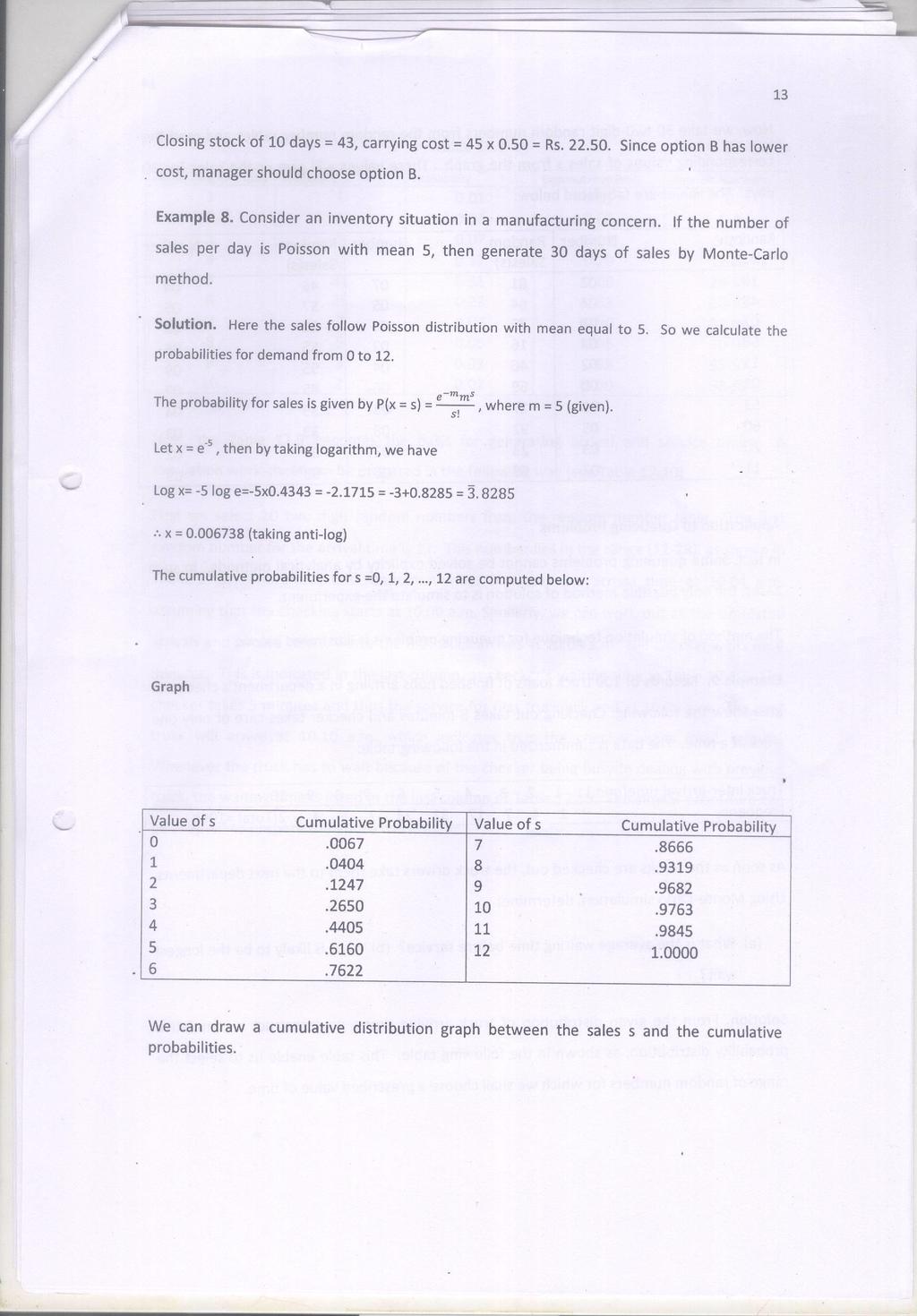
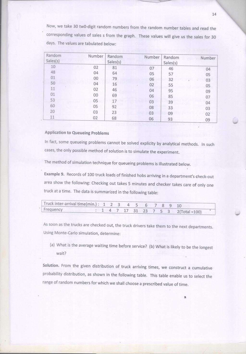
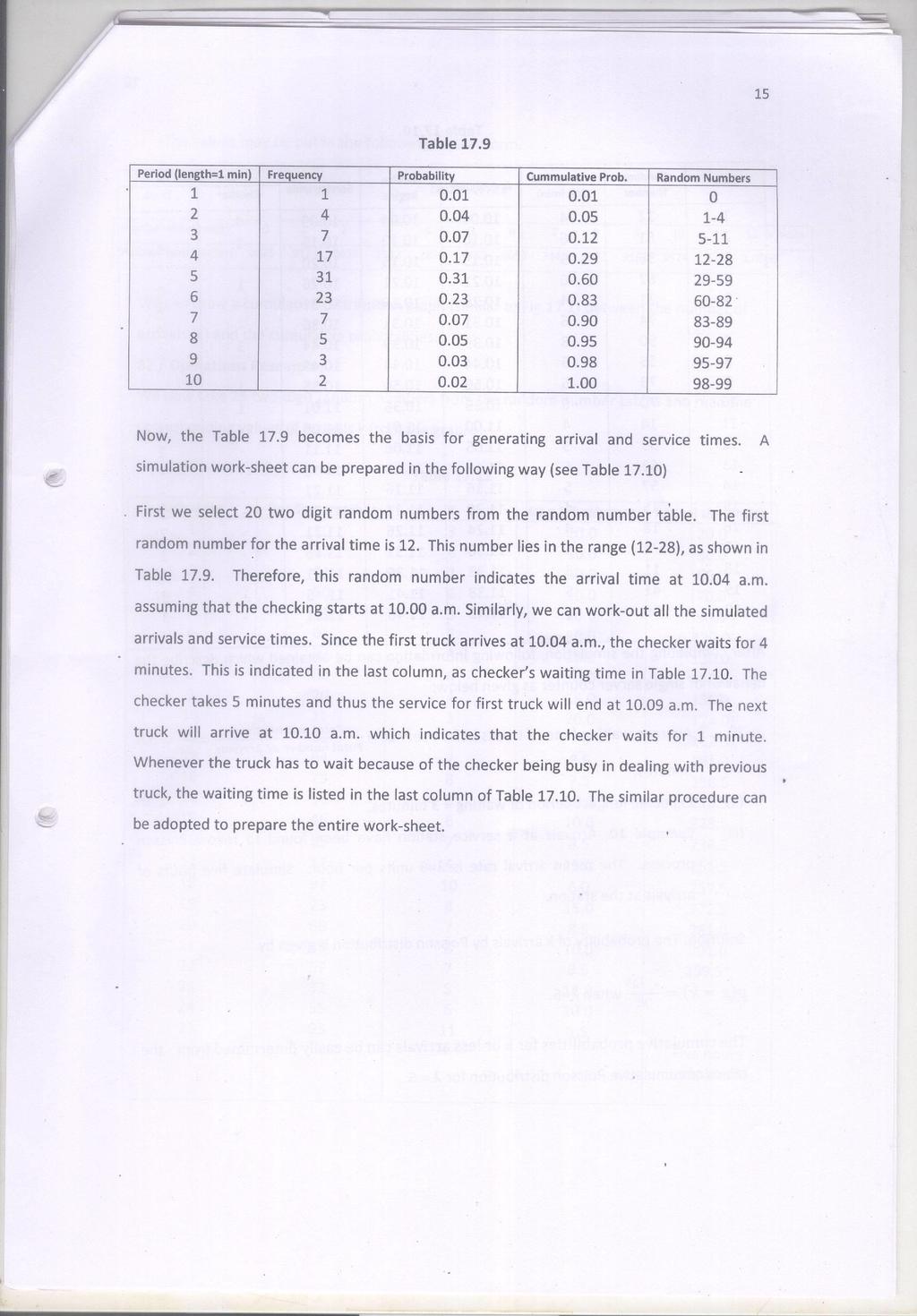
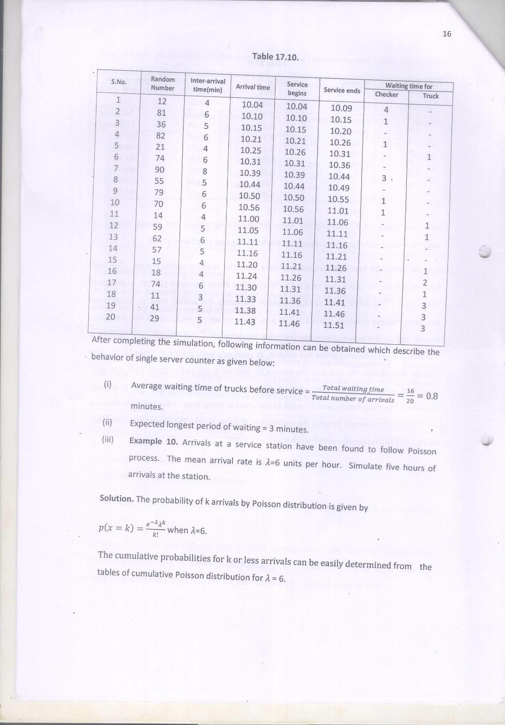
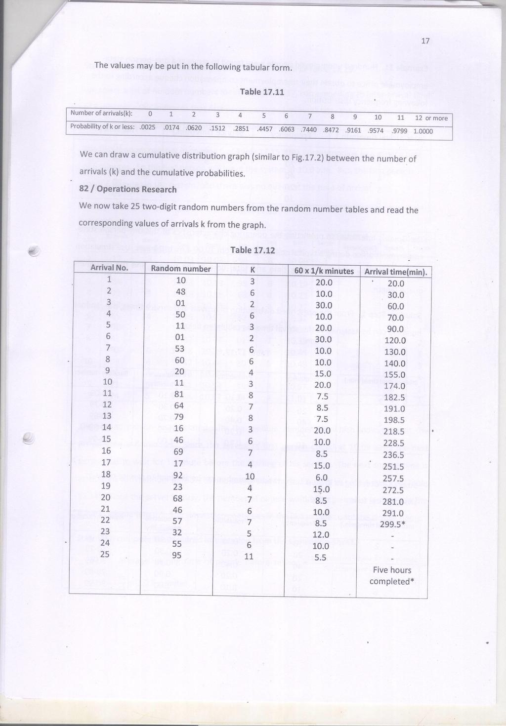
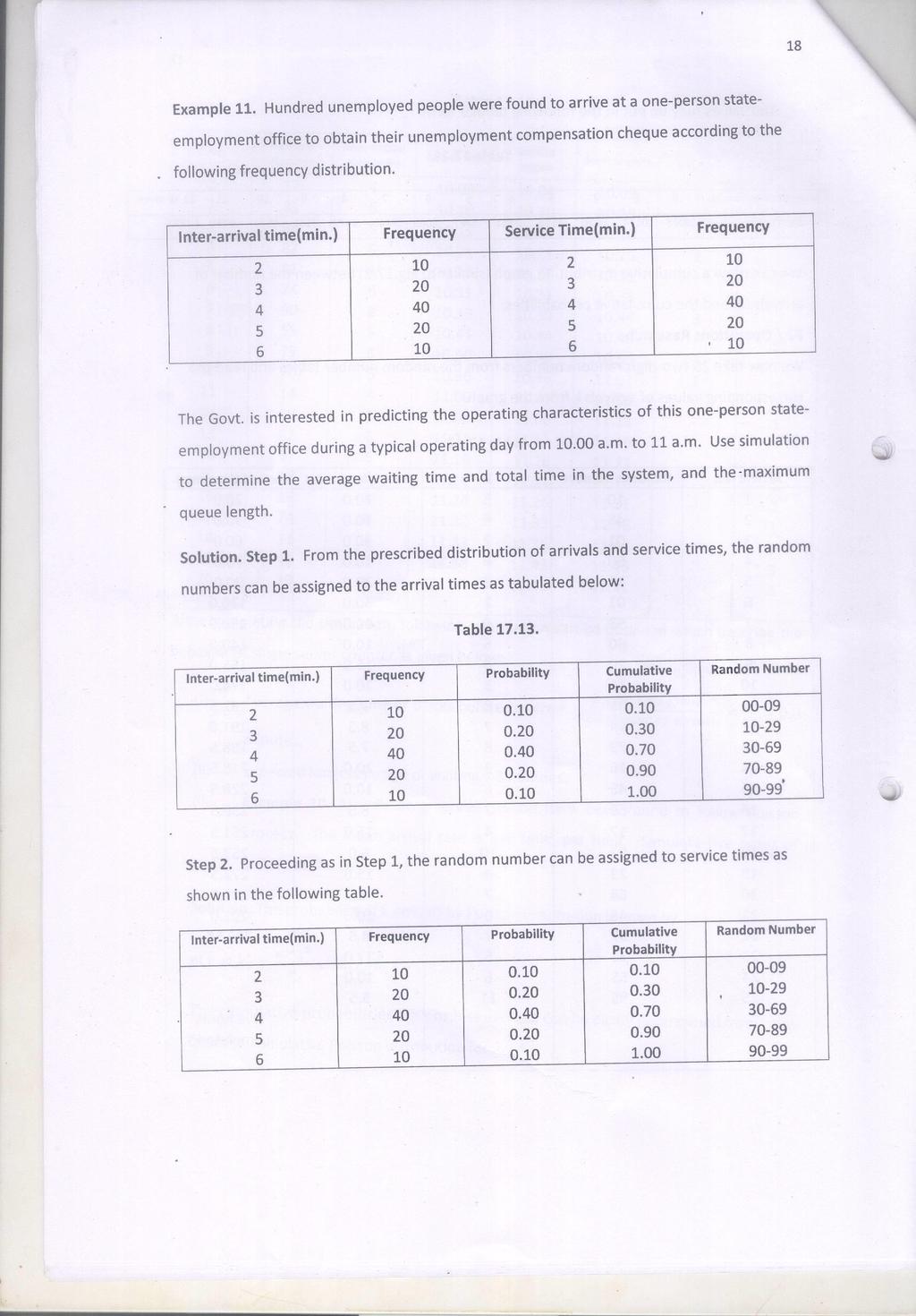
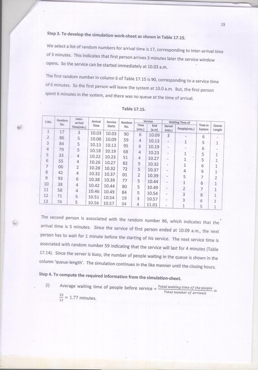
47 UNIT VIII SIMULATION

48

49

50

51

52

53

54

55

56

57

58

59

60

61

62

63