Developing an Interactive GIS Tool for Stream Classification in Northeast Puerto Rico

Transcription

1 Developing an Interactive GIS Tool for Stream Classification in Northeast Puerto Rico Lauren Stachowiak Advanced Topics in GIS Spring

2 Table of Contents: Project Introduction Project Overview Page 3 2. The Study Area Page 4 3. The Datasets Used Pages 5-6 Table of Contents: In-Situ Model Model Introduction Page 7 2. Branch 1: Flow Hydrology Pages Creating Waterhseds Page Branch 2: Meshing Polygons Page Final Steps: Stream Classification Page ArcScene 10 Screenshots Pages Table of Contents: Upstream Model Model Introduction Page Isolating Subclasses Page Draining and Calculating Dominance Pages Final Steps: Stream Classification Page ArcScene 10 Screenshots Pages The Wrap Up: Conclusions and Weaknesses (22-24) ArcScene 10: Landscape Flyovers (25)

3 Project Overview This project aimed to answer basic environmental questions about a tropical montane ecosystem. Two models were created to classify streams flowing within the study area based on specific environmental parameters used as inputs. The output of each model is a derived vector stream network, which has as data within the attribute table the identification of each parameter, given as inputs, on a per stream reach basis. The input parameters used for each model were a bedrock lithology layer and a vegetation layer. For the first model, the in situ environment surrounding the stream reach was used to classify each stream. For the second model, the upstream dominance of each parameter (bedrock and forest type) were applied to the downstream channel reaches. Both models relied on vector and raster data as inputs. This GIS project was tailored around my MES thesis and was used to enhance the methodology and techniques section of the final paper. The main goal behind this project was to generate a more applied GIS focus to my thesis and to better understand the flow hydrology toolset. In addition, I wanted to investigate how models could be created to automate certain processes. The focus of my thesis revolved around potential influences in drainage density patterns as influenced by bedrock and vegetation, which is why I have chosen those particular datasets for this project. Lastly, I have chosen to create my final project for this class in a.pptx format because it contains many graphics, which are better displayed and oriented in a slide rather than in a word document. The following sections within this document describe how a potential user can execute the model and steps to take for proper model use. To begin, a brief overview of the study area and data used in the model creation is explained. 3

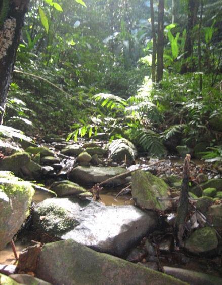
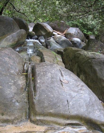
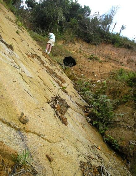
4 The Study Area The study area for this project is the Luquillo Mountains located in northeast Puerto Rico. It is classified as a humid, tropical montane ecosystem. The geographic coordinates are: Lat: N and Long: W. Quick Stats: Peaks at 1060 m >5000mm of precip/year Average annual temp. of 73 F Only tropical forest in USFS 4

5 The Datasets: Introduction This project begins with three base data layers, which are then used to generate several consecutive layers of data. The data are composed of a digital elevation model (DEM), a polygon shapefile of vegetation boundaries, and a polygon shapefile delineating bedrock lithology. The following images show these data layers and the corresponding attribute tables. Base Layer 1: DEM HIGH LOW This layer will be used to derive the vector stream network in later steps. This DEM is a raster data layer based on a 10 meter cell resolution. Since the cells are floating point integers in raw form, there is no attribute table. However, the region as a total of 1051 m relief, with a peak of 1060 meters and lowland of 9 meters. The data was acquired from Miguel Leon and the LCZO research group. 5

6 Base Layer 2: Vegetation The attribute table represents information for each feature in the polygon shapefile. The vegetation consists of 4 classes: tabonuco (red), colorado (yellow), elfin (dark green), and palm (light green). The forests occupy a total of 42 watersheds. Base Layer 2: Bedrock Lithology As you can see, this shapefile is very similar to the vegetation layer. There are three geology classes including: volcanic (purple), quartz diorite (green), and hornfels (blue). There are 42 watersheds in this area as well. Area was calculated here as well in (m/ha) Both vector layers above have been overlayed with a hillshade layer to better show relief. Symbology of each layer will be kept constant throughout this document. 6

7 In Situ Cartographic Model This first model assigns environmental classifications to stream reaches within the immediate surrounding area (polygonal boundaries) of each corresponding bedrock/vegetation parameter. Essentially, those polygons through which the streams flow will be the ones whose classifications will be applied to each reach. The following pages explain in more detail the below steps written in the tool: I. Generating the stream network with stream order preserved using a DEM of the study area. II. Generating a watershed shapefile consisting of a constant surface of polygons III. Meshing Polygons and Classifying Streams The below model is shrunk to show completely on this slide. It will be broken down in the following slides. *This is what the tool looks like in ArcMap Model Inputs: 1. DEM 2. Watershed Data; allows the user to define their own watersheds based on site-specific field observations. 3. Two environmental parameters. Each must be polygon vector files and must occupy the same space as the DEM and watershed layers. 7

8 I. Deriving A Vector Stream Network A B C All flow sinks in the original DEM were filled with the Fill tool to make this output file. D Flow Direction was calculated for each cell giving values representing cardinal directions. E Flow Accumulation was calculated from the direction raster to find flow channels. F A threshold of 50 was set to limit the network using Raster Calculator. Stream Order was calculated giving each stream a reference number. A vector file was created using the Stream to Feature tool. A B C D E F The tools used in this first branch of the model are shown in bold. 8

9 A Closer look at Flow Direction Considering that many future operations in this model and the second model rely on this raster data layer, it is worth taking a closer look at this hydrology operation. Essentially, this tool looks at the DEM (or the filled DEM) on a pixel-by-pixel basis and assigns each cell a value based on the direction to the steepest immediate neighbor. The new cell values will be one of eight cardinal directions. Below the flow direction raster from the previous page is shown in planimetric and perspective view (from ArcScene). On the right, is the direction raster converted to points and symbolized with rotating arrows to better show what the computer sees when it uses the direction raster for the next step in flow accumulation. It has been overlayed on a DEM to simply show background perspective (so the arrows aren t floating in space). Notice distinct V-shape valleys on all three pictures. 9

10 II. Creating a Site-Specific Watershed Layer A point shapefile of pour points was manually created (green circles) to represent where the water drains. These represent the outlets of each watershed. The pour points were placed at the junctions of bifuracted streams outside of the park to generate a constant surface throughout the entire study area. The watershed tool requires the direction raster and the pour points for operation. The watershed layer was converted to a vector polygon file and the attribute table to the left shows the features in the layer. The final watershed count for this particular study area was a total of 42 watersheds. *Your watershed layer would look different than this one. 10

11 Watersheds Geology Vegetation III. Meshing Polygons These three vector layers, shown on the left, are meshed together into a single polygon layer. This is done by a series of nested intersections, which allow this final polygon layer (shown below) to assume the classifications of each of the three starting layers. Just as a reminder, when running this model for your particular study area, this final polygon layer will look different based on your own data. 11

12 IV. Final Steps: Stream Classification The final stream network, shown in red to the left, has been intersected with the polygon layer from the previous page. It was overlayed with a semitransparent hillshade and watershed layer to show individual basins and relief. The attribute table shown below is for the stream reaches selected from the network (shown in light blue on the map). 12

13 ArcScene 10 Screenshots The following images are a sample of screenshots taken throughout the creation of this model. They are meant to give better visual representation of the study area and the different layers used as inputs and those created during model execution. This is a schematic made with layered raster datasets created in the flow hydrology branch of the model. The bottom is a DEM and the top is the derived stream network. The top image is an oblique view of the stream network with the geology layer. The bottom is the classified streams draped on a 3D landscape (the filled DEM). 13

14 Above is the same example as the geology layer, but now with vegetation. The top right and bottom images are views of the study area. The top image is a bird s eye view from the NE looking SW, the bottom is at a horizon level looking due north. 14

15 Upstream Cartographic Flow Model This second model classifies stream reaches based on the dominance of bedrock and vegetation types from the upstream catchment areas. Essentially, each environmental subclass is drained down the DEM surface and total accumulation values are calculated on a pixel basis. These values are then attributed to stream reaches on a majority ranking system, where each stream is given the bedrock and vegetation type most dominant upstream. The flow hydrology branch of the model is the same as the first model, so it will not be described again here. As you can see, this model is more complicated and requires many more steps. The following procedures will be discussed in the following pages: I. Isolating the environmental parameters based on subclasses of data II. Draining these isolated subclasses and accumulating flows III. Calculating Upstream Dominance and Classifying Streams 15

16 I. Isolating Environmental Parameters Each input vector polygon layer must be broken up into individual data layers based on their subclasses. This step in the model is done after the polygons have been converted to raster, by way of a series of reclassifications. The output rasters are 0/1 grids with 1s representing previously defined subclass extents and 0s being those areas previously belonging to the other subclasses. (ie. in the geology layer there are three subclasses, so three 0/1 grids are generated). The tools to take the vector polygon layer of bedrock lithology distributions to the left and get the three 0/1 grids below are as follows (the steps are the same for vegetation): 1. Convert to Raster 2. Reclassify. This was done 3 times for geology and 4 times for vegetation (not shown) for a total of 7 reclassifications. From left to right the three grids immediately above are volcaniclastic, quartz diorite, and hornfels. Red = 0, and Blue = 1 for all three grids. 16

17 II. Draining and Accumulating Subclasses Each of the seven 0/1 grids created in the isolation operations from the previous page were then drained down the DEM landscape using the flow accumulation operation. The flow direction raster is used and each 0/1 grid is used as the weight raster. Each of the flow accumulation grids on the left have cell values representing total upstream cell counts attributed to that rock type. Using Cell Statistics, the 3 datasets are added together to get total upstream cell counts for all rock types. The flow accumulation grids are overlayed with the transparent geology layer. 17

18 III. Calculating Dominance Values Per Subclass The first step to determining dominance is to calculate the relative percentage of total upstream accumulation belonging to each rock type. This is done three times with the expression shown in the dialogue box. The next step is to take each raster calculator output, here labeled catch_rocktype, and run the highest position operation. The output shown below has cell values which identify which rock type is most dominant on a pixel-bypixel basis. Order of inputs is important here. 18

19 IV. Stream Classifications The stream classification steps are similar to those in the first model. Each highest position output grid from the previous page for both initial input datasets (bedrock and vegetation) are then converted to polygons. These two polygon layers are first intersected with each other, and then to the stream network derived from the flow hydrology branch. Polygons on the left create the networks to the right. The streams to the right are symbolized based on the dominant upstream rock type (top) and vegetation (bottom). 19

20 ArcScene 10 Screenshots The left image is taken from the N looking S. It shows tabonuco (red), colorado (yellow), palm (light green), and elfin (dark green) streams. Notice how some streams bleed outside of the natural distributions of their bedrock type. Both colorado and palm streams are shown in the tabonuco boundary. The bottom image is a landscape view taken from a horizon perspective looking due north. 20

21 The image to the left was taken in Arcscene showing a stream layer that has been overlayed with a transparent geology layer. Again, notice how the hornfel (blue) streams are found in quartz diorite (green) and volcaniclastic (red) distributions. The bottom image is a landscape view of the stream network taken from the NW looking SE. You can see here also, how the streams flow further downslope. 21

22 GEOLOGY VEGETATION The Wrap Up: Conclusions Below are the output stream networks from both models. Shown are stream reaches based on geology and vegetation separately to compare some areas where the networks differ. MODEL 1 MODEL 2 22

23 The Wrap Up: Model Weaknesses I. MODEL 1 1. Environmental Data must be in the form of vector polygons 2. The second parameter is required. The model must compare two separate parameters. It would be beneficial to make the second optional. 3. The critical contributing area threshold must be known before model is run and currently the area is set as all cells with an accumulation cut-off of ln(4) or higher.

24 II. MODEL 2 1. This model also requires vector polygons as inputs for the environmental parameters. 2. As of right now, a big weakness is that one parameter must have four variables, and the other must have three, and they must be used as the right input parameter for the tool. 1 2 As you can see, this model was built specifically with the bedrock and vegetation data in mind so that it would ultimately run properly. However, as a result of this, environmental parameter 1 must have exactly 3 subclasses and environmental parameter 2 can have only 4 subclasses of data. This really is not a practical assumption to make of some other user s future data. 24

25 ArcScene 10 Study Area Flyover Here is where the flyover video would be if it were not over 20 MB in size. Because I can only send s with a max size of 25MB, I will the video to you separately. The flyover is of the first model with the stream network symbolized by both bedrock and vegetation (3 rock types and 4 vegetation types = 12 possible combinations of subclasses). There are twelve different color schemes, one for each possible rock/veg combination. The video transects the study area from the SW over one river valley into a second in the NE. 25