National Center for Airborne Laser Mapping. Airborne LIDAR Data Processing and Analysis Tools ALDPAT 1.0

Transcription

1 National Center for Airborne Laser Mapping Airborne LIDAR Data Processing and Analysis Tools ALDPAT 1.0 Keqi Zhang 1,2 & Zheng Cui 1 1 International Hurricane Research Center 2 Department of Environmental Studies Florida International University Miami, FL April 2007

2 Table of Contents 1. INTRODUCTION FRAMEWORK FOR PROCESSING LIDAR DATA PROGRAM DETAILS... 5 Graphic User Interface... 5 Other Software Needed... 7 Organization of Files... 7 Set up of Delimiter for Output DESCRIPTION OF TASKS... 9 Task 1. Split Tape Files into Strips... 9 Task 2. Separate First and Last Return Measurements from a 9 Column Strip File Task 3. Convert ellipsoid to orthometric heights Task 4. Estimate strip boundary Task 5. Merge Boundary Files Task 6. Create Shape File Task 7. Tile Strips Task 8. Filter LIDAR Points Elevation Threshold with Expand Window (ETEW) Progressive Morphology (PM) D Morphological Filters (Square or Circle Window) Maximum Local Slope (MLS) Iterative Polynomial Fitting (IPF) Polynomial Two-Surface Filter Adaptive TIN (ATIN) Task 9. Gridding Tiles Task 10. Convert Surfer Grids to ArcGIS Grids Miscellaneous Tasks Reduce Point Density Extract Points by Polygon APPENDIX. BRIEF DESCRIPTION OF FILTERING ALGORITHMS Elevation Threshold with Expand Window (ETEW) Filter Progressive Morphological (PM) Filter Iterative Polynomial Fitting (IPF) Filter Adaptive TIN (ATIN) Filter REFERENCES ii

3 List of Figures Fig. 1. Schematic procedure for LIDAR data processing... 3 Fig. 2. Example of 9 column data... 9 Fig. 3. A boundary polygon for a strip Fig. 4. Tiles for a LIDAR data set Fig. 5. A tile with a buffer Fig. 6. Tiles for a long and narrow area Fig. 7. Diagram of Grid Fig. 8. A sample of tile_parameter.txt Fig. 9. A polygon overlaying an elevation grid interpolated from LIDAR measurements in ArcGIS Fig. 10. Extracted points within the polygon Fig. 11. Measures used to separate ground and non-ground LIDAR points Fig. 12. Examples of raw and filtered LIDAR points using ETEW filter Fig. 13. Process of the progressive morphological filter to identify terrain and building measurements Fig. 14. Profile illustrating the filtering process of local polynomial fitting method Fig. 15. Filtering processes for the polynomial two surface filter Fig. 16. Selection of ground points in ATIN filter iii

4 1. Introduction High resolution digital terrain models (DTMs) and digital surface models (DSMs) are critical for predicting flooding, monitoring erosion, landslide and tectonic movements, modeling ecosystems, and creating digital city models. Recently emerging airborne light detection and ranging (LIDAR) technology allows accurate and inexpensive measurements of topography, vegetation canopy heights, and buildings over large areas. In order to provide researchers with high quality data, NSF has created the National Airborne Laser Mapping Center (NCALM) to collect, archive, and distribute the LIDAR data. However, airborne LIDAR systems collect huge volumes of irregularlyspaced, three-dimensional point measurements of ground and non-ground objects scanned by the laser beneath the aircraft. To advance the use of the technology and data, there is a need for basic research in algorithms for data retrieval and transformation, and ground and non-ground measurement classification. There is also a need for additional software which includes these algorithms and other basic data processing tools to help researchers to extract the desired information from airborne LIDAR data for their applications. In order to satisfy these needs, we have developed a set of transparent and automatic filtering algorithms to classify ground and non-ground LIDAR measurements and a series of auxiliary tools such as thinning, tiling, and gridding the point data sets to assist the LIDAR data analysis. A graphics-based user interface has also been developed to facilitate the usage of algorithms and tools. We hope that the algorithms and software will provide researchers with the necessary tools to analyze LIDAR data and derive useful information in order to understand and model natural and human-induced earth surface processes and their changes. We also hope that the LIDAR data processing and analysis tools will help promote the scientific, government, and the public s use of LIDAR data and technology to predict topographic effects of major earthquakes, large scale flooding, extensive landslides, and erosion. These algorithms and tools were developed through the cumulative efforts of the authors in airborne laser mapping research during the past eight years. We would like to thank NCALM and NOAA Florida Hurricane Alliance Research Program for providing the necessary financial support for this project. Mr. Quin Robertson and Ms. Patricia Houle at Florida International University tested the software and provided valuable feedback. 2. Framework for Processing LIDAR Data Developing the tools to process LIDAR data is a challenging task because of the unique characteristics of LIDAR data. A LIDAR data set consists of huge volumes of irregularly spaced points, making it difficult to directly analyze the data in commercial GIS and remote sensing software which are designed to handle vector and raster images. Processing of raw LIDAR data using such methods as coordinate transformation, tiling, or gridding is needed to prepare the data for a further analysis in GIS and remote sensing software (Fig. 1). The data processing starts from the nine column tape data generated by NCALM LIDAR system-optech ALTM 1233 and ends at the generation of digital terrain models (DTMs) or digital surface models (DSMs). In addition, raw LIDAR points include measurements for terrain and non-terrain objects such as vegetation, buildings, and cars. Ground and non-ground measurements 1

5 have to be separated in order to produce DTMs. One possible solution is to generate raster images by interpolating raw LIDAR measurements so that existing raster image classification and feature extraction methods can be used. However, interpolation can introduce errors into the LIDAR data set. It is preferred to classify LIDAR measurements at the point level so the users can use appropriate methods to process the data further to fit their application best. Many algorithms have been developed to separate ground and non-ground LIDAR points, a process also called as LIDAR data filtering. The rationale for these algorithms is that elevation change of terrain is usually gradual in a neighborhood, while the elevation change between buildings or trees and the ground is very large. This difference in elevation change is used to construct measures for separating ground and non-ground measurements. The measures include local slope, height range, and distance to a locally fitted surface (Sithole and Vosselman, 2004; Zhang and Whitman, 2005). However, there are some special geomorphic forms such as bluffs/cliffs and sand dunes which also have large elevation changes. The LIDAR measurements for these features could be mistakenly classified in terms of the separation measures. On the other hand, low and dense vegetation in high relief areas with large slopes can be incorrectly classified into ground points. There is no magic filter which can identify all landforms without errors because of the complexity of the earth surface. All existing filtering algorithms suffer commission and omission errors in various degrees, depending on their measures and types of topography, vegetation, and buildings. Filter comparison studies showed that existing algorithms performed well in landscapes of low complexity in general, while very small objects (e.g., vehicles), landscapes with complex shape/configuration (terraces), and disconnected terrain (courtyards) pose a great challenge for classification (Sithole and Vosselman, 2004). Based on the current status of filtering algorithm development, our strategy is to implement various filters with transparent algorithms. Transparent classification algorithms facilitate the interpretation of results and error analysis. Researchers can select the filters which best fit their applications. The filtering tools and a series of auxiliary tools consist of the following 10 major tasks and miscellaneous tasks for the data processing framework: 1. Split Tape Files into Strips 2. Separate First and Last Stop Measurements from a 9 Column Strip File 3. Convert ellipsoid to orthometric height 4. Compute strip boundary 5. Merge Boundary Files 6. Create Shape File 7. Tile Strips 8. Filtering LIDAR Data 9. Gridding Tiles 10. Convert Surfer Grids to ArcGIS Grids 11. Miscellaneous tasks The procedures to perform each task are illustrated in the following sections. A schematic for the LIDAR data processing tools is shown in Fig 1. 2

6 Fig. 1. Schematic procedure for LIDAR data processing. 3

7 Fig. 1(cont.). Schematic procedure for LIDAR data processing. 4

8 A graphic user interface based software system will greatly help researchers who do not have much programming experience to use LIDAR data processing tools. We took a two-tiered approach to develop the algorithms and graphic user interface. Major algorithms were implemented in a standard ANSI C++ environment at the back end to optimize computing performance. The graphic user interface (GUI) was developed to take the input parameters from users and call the algorithms to perform computations. The GUI was developed for the Microsoft s Windows platform considering the popularity of personal computers. 3. Program Details Graphic User Interface There are two important menu items in the GUI: Settings and Tools. The menu item Preference under Settings is used to set up the output format and the location of installed Corpscon (see below) software. The menu item Worksheet under Tools is used to select input files, output directory, processing method and show the processing status. 5

9 All the methods in the Work Sheet can be run as either single or multi-files. Once the file is processed successfully, the message box will display Success, and Status will change from Ready to Done. Otherwise, an error message will be displayed in the message box. Different jobs can be processed in the Work Sheet after parameters for each job are set up and added to the Work Sheet using the Add New Jobs button. You can delete jobs in Ready or Done status by selecting target rows first and then clicking Delete Jobs button. You can select a single row in the work sheet by clicking the left button of the mouse and select multi-rows by clicking the left button of the mouse and pressing Ctrl or Shift key simultaneously. 6

10 Other Software Needed For some of the tasks included in the Airborne LIDAR Data Processing and Analysis Tool, other software programs are needed to process or display the data. A list of software is shown below. More details can be found in the descriptions for the appropriate tasks. Task 3: Convert Ellipsoid to Orthometric Heights U.S. Army Corps of Engineers Corpscon Version 6.0 Task 6: Create Shape File ESRI ArcGIS for displaying results Task 9: Gridding Tiles Golden Software Company Surfer 8 Task 10: Convert Surfer Grids to ArcGIS Grids ESRI ArcGIS for viewing results Organization of Files Since the operation of this tool produces many data files at each step, it is recommended that a structure of file names, folders and directories be set up in advance. Using Fig. 1 as a guide, an example is shown below. Although the program appends task-specific suffixes to processed files, it is best to decide on naming conventions ahead of time. 7

11 Set up of Delimiter for Output This task sets up a delimiter for text formatted output files. Both comma and space delimited colonized data can be read from and written into the files by the software. 1. Select Preference from Settings menu 2. Select the delimit for the output file 8

12 4. Description of Tasks Task 1. Split Tape Files into Strips This task is designed for separating LIDAR data for various strips. The input file includes an aggregated ASCII file from Optech REALM software which includes 9 column LIDAR data for several strips. The format for each record (row) of the aggregated file is assumed to be t, x 2, y 2, z 2, i 2, x 1, y 1, z 1, i 1 (Fig. 2). Here, x 2, y 2, and z 2 are horizontal and vertical coordinates, and i 2 is the intensity of a last return point; followed by x 1, y 1, and z 1 which are horizontal and vertical coordinates, and i 1 the intensity of a first return point. We assume that the 9 column data in the file follow this format. In order to facilitate data processing, make sure that you output the data from OPTECH REALM using this format. Other output format from REALM such as t, x 1, y 1, z 1, i 1, x 2, y 2, z 2, i 2 can be selected too. If you select the different output formats, make sure that the positions of first and last return data in the input files match those in the output files. Fig. 2. Example of 9 column data. Since the laser is turned off between two adjacent strips, the time interval computed based on t for current and previous records in a 9 column data set is used to determine the separation of strips. If the time interval is greater than a given threshold value (i.e., 60 seconds), a new strip file is generated. The output format of the strip file is the same as the input file, i.e., t, x 2, y 2, z 2, i 2, x 1, y 1, z 1, i Select WorkSheet Since input parameters for all ten tasks are set up through the WorkSheet, a task always starts with opening the WorkSheet. The WorkSheet can also be opened using the icon located on the toolbar. 9

13 2. Select input files and output directory 3. Select data processing method 10

14 4. Add a new job 5. Select parameters Interval: time interval between two strips. 11

15 6. Run the job 7. Results 12

16 Task 2. Separate First and Last Return Measurements from a 9 Column Strip File This task separates first and last return measurements from 9 column ASCII data. The format for each record (row) of the 9 column data is assumed to be t, x 2, y 2, z 2, i 2, x 1, y 1, z 1, i 1. Here, x 2, y 2, and z 2 are horizontal and vertical coordinates, and i 2 is the intensity of a last return point. x 1, y 1, and z 1 are horizontal and vertical coordinates, and i 1 is the intensity of a first return point. 1. Select WorkSheet 2. Select input files and output directory 13

17 3. Select method 14

18 4. Add new jobs 5. Select parameters 15

19 UTM Zone: UTM zone number may be included for x and y coordinates in the 9 column data, select the appropriate UTM zone number in order to remove the number from x and y coordinates. If the 9 column data do not include the UTM zone number, just use the default value. The program automatically determines whether the UTM zone number is included in the x and y coordinates in terms of number of digits. Stop Gap: Small footprint laser systems such as the ALTM 1233 used by NCALM need to generate sufficient energy per pulse to obtain return signals strong enough to be sensed. On the other hand, to avoid damaging optical components and comply with eye-safety-regulations, a narrow pulse with high energy cannot be used. Therefore, the laser pulse widths used by an airborne LIDAR system typically spread about 10 nanoseconds for safety reasons, a time equivalent to 3 meters in distance. This implies that theoretically the last return measurement is not reliable if the difference between the first and last returns is less than 3 meters. We found that 5 meters is a good threshold through data processing experiments. If the elevation difference between the first and last return measurements is less than 5 meters, the last return measurement is replaced by the first return measurement. Of course, you may enter any number into the Stop Gap field. Fields: XYZI is for output with x, y, z coordinates and intensity; XYZ is for the output with x, y, and z coordinates only. 6. Run the job 16

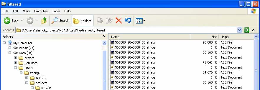
20 7. Job status 8. Results The first and second stop files and the log file will be placed in the same directory. For future processing, it is recommended that you move the second stop files (identified by the suffix _2 ) into the appropriate directory. The log file lists the parameters used for the method. 17

21 Task 3. Convert ellipsoid to orthometric heights U.S. Army Corps of Engineers software Corpscon (Version 6.0) is an MS- Windows-based program developed by the U.S. Army Corps of Engineers, which allows the user to convert coordinates between Geographic, State Plane, Universal Transverse Mercator (UTM) and US National Grid systems on the North American Datum of 1927 (NAD 27), the North American Datum of 1983 (NAD 83) and High Accuracy Reference Networks (HARNs). Corpscon uses the National Geodetic Survey (NGS) program NADCON to convert between NAD 27, NAD 83 and HARNs. Corpscon performs vertical conversions between the National Geodetic Vertical Datum of 1929 (NGVD 29) and the North American Vertical Datum of 1988 (NAVD 88). Vertical conversions are based on the NGS program VERTCON and can only be performed for the continental U.S. Corpscon can also calculate geoidellipsoid separations based on the NGS program GeoidXX (XX = 90, 93, 96, 99, and 03). Geoid-ellipsoid separations can be calculated for the Continental U.S., Alaska, Hawaii and Puerto Rico/U.S. Virgin Islands. Since Corpscon does not provide a batch function to process multiple files, users have to deal with each input file one by one. It is inconvenient for the users to perform a conversion for large numbers of files, which is a typical case for LIDAR data processing. However, Corpscon provides a dynamic link library (DLL) named corpscon_v6.dll for users to integrate conversion functions into their own program. We have integrated most of the conversion functions of Corpscon into the NCALM LIDAR data processing program to provide a batch function to convert multiple files. Our program loads the DLL at runtime to call the functions for data conversion. In order to perform data conversion, Corpscon can be downloaded at and has to be installed at C:\Program Files\Corpscon6\ 1. Select method Corpscon You can add a suffix to every output file to differentiate names for input and output files. If you do not add a suffix, a default suffix (e.g. Corp ) will be added to output file names 18

22 2. Set up datum transformation parameters Note: Input and Output Zone format here is: UTM zone No. range of longitudes for that UTM zone, hence 17-84W to 78W. 3. Run the job 19

23 4. Results For each strip the default suffix _Corp is added to the input file name. A log file is also produced and shows the input and output parameters. 20

24 Task 4. Estimate strip boundary Strip boundaries (Fig. 3) need to be examined to determine the completeness of a LIDAR survey and the overlapping percentage between strips. The following algorithm has been created using 2D array to extract the strip boundary by: Creating a mesh with a fixed cell size overlaying the data set Assigning each point measurement from the LIDAR data set into a cell in terms of x and y coordinates of the point. If more than one point falls in the same cell, one with the lowest elevation is selected as the array element Deriving minimum and maximum x and y coordinates for the whole data set If x max -x min y max -y min, deriving a pair of points with minimum and maximum x for each row of the array. If x max -x min <y max -y min, deriving a pair of points with minimum and maximum y for each column of the array. Output the boundary points for each row or column for further processing Fig. 3. A boundary polygon for a strip. The boundary polygon is generated by connecting points in boundary cells. 21

25 1. Select method Get Strip Boundary 2. Select input files 22

26 3. Select output directory 4. Add new jobs by clicking Add New Job button 23

27 5. Set up parameters Width: cell width of the mesh covering the whole data set Height: cell height of the mesh Scan Direction: search direction for deriving boundary. This parameter can be set into x, y, or automatic. If the parameter is set to be automatic, the search direction will be determined by comparing the range of x and y as described in the algorithm 6. Run the job 24

28 7. Results Output are x, y, z, intensity for points at the boundary of a strip The default suffix _Bound is appended to each input file. A log file showing input parameters for each file is also produced. 25

29 Task 5. Merge Boundary Files It is convenient to convert boundary files for strips in a survey area into an ArcView shape file for display purposes. In order to do so, the boundary files which you would like to convert into a shape file have to be combined together first. 1. Select the method Merge Boundary 2. Select input files 26

30 3. Type output file name For this task, you need to explicitly name the output file. 4. Add new job and run the job 27

31 5. Results The result is a 5-column text file showing x, y and z coordinates, which strip contains the coordinates and the name of the input file. Note that separates the strips. The log file shows the merge boundary parameters. 28

32 Task 6. Create Shape File The program ArcGIS (ESRI) is needed for displaying the result. 1. Select the method ESRI Shape and select merged boundary file as input 29

33 2. Select output directory and file name 3. Add new job and run the program. Accept the default values on the parameter screen. 30

34 4. Load shape file into ArcGIS so you can see the area covers by the strips and determine the range for tiling. The shape file produced does not include a projection file (.prj). Use ArcCatalog to define the projection. Record the minimum and maximum X and Y values for the shape file. They need to be input as integers in Task 7. 31

35 Task 7. Tile Strips Since a LIDAR data set often includes millions, even billions of point measurements, it is very difficult to display and analyze the whole data set using a single file. We can split the data set into tiles to facilitate the data processing (Fig. 4). Tiles can be organized following the system of existing data sets such as the USGS quad sheets. Fig. 4. Tiles for a LIDAR data set The size of a tile is determined by the point density and the capacity of the users computers. A tile with a cell size of 2 km is recommended for the NCALM 1233 ALTM data set. In addition a buffer around the tile (Fig. 5) is often created to ensure the consistency of filtering, gridding, and merging. Fig. 5. A tile with a buffer. 32

36 1. Select the method Tile and select strip files as input (from Task 3) 2. Select output directory It is recommended that you create a new directory to store the tiling results. 33

37 3. Select tiling parameters \ Width: width of a tile along x axis. Height: height of a tile along y axis. Tile Direction: tiling method. XY is for tiling the data along both x and y direction; both x and y coordinates are incremented in terms of width and height of the tile. X is for tiling the data along x direction. Only x coordinates are incremented for tiles and y coordinates for each tile is the minimum and maximum value of y coordinates for the entire data set. Y is for tiling the data along y direction. Only y coordinates are incremented for each tile and x coordinates for each tile equals to the minimum and maximum value of x coordinates of the entire data set. If the data cover a large area, it is recommended that the data set be cut into square or rectangle tiles through XY direction. If the LIDAR surveys cover a long and narrow area, it is recommended to cut the data by selecting only the x or y direction. Buffer Size: buffer size for a tile. Min and Max X Y: the method to determine minimum and maximum x and y values for each tile. Minimum and maximum x and y values can be derived by manually measuring the boundary shape file in ArcGIS (see slides for task 6). If users do not set up minimum and maximum x and y manually, the program will select the minimum and maximum x and y values automatically in terms of a minimal rectangle covering all strips in a floating point format. The manual selection of x and y ranges are recommended because integer values are preferred for the minimum and maximum x and y values. Min X: minimum x coordinate for the entire data set. Max X: maximum x coordinate for the entire data set. Min Y: minimum y coordinate for the entire data set. Max Y: maximum y coordinate for the entire data set. 34

38 Fields: XYZI each row of the output data includes the x, y, z coordinates and intensity value of a point measurement. XYZ each row of the output data only includes the x, y, and z coordinates of a point measurement. 4. Run the jobs 5. Results 35

39 Note: Tile parameter files include minimum and maximum x and y values for each tiles and will be used in the gridding processes. A tile file is generated by appending all points falling within the tile boundary from different strips. If you tile a strip twice, the data will be appended to the tile file twice. If you would like to retile your data, you have to delete the old tile files first to avoid repetitive data in the tile files. When tiling the data along Y (Fig. 6), we use the same procedure as cutting the data along XY direction. However, the tile direction is set to be Y. The Min X and Max X is set to be the minimum and maximum x values of the entire data set. The value of width in the input parameter table is ignored during tiling process. Fig. 6. Tiles for a long and narrow area. Input parameters for tiling the data along Y direction 36

40 Results Tile_paramater.txt: Tiling the data along X direction is similar to tiling the data along Y direction. 37

41 Task 8. Filter LIDAR Points Several algorithms have been developed for this LIDAR data processing software to classify the ground and non-ground LIDAR measurements. Details of each algorithm can be found in the Appendix. The algorithms described here are: Elevation Threshold with Expand Window (ETEW) Progressive Morphology (Morph Filter) 2D Morphological Square (Morph 2D Filter) 2D Morphological Circle (Morph Circle Filter) Maximum Local Slope (Slope Filter) Iterative Polynomial Fitting (Polynomial Filter) Polynomial 2 Surface Filter Adaptive TIN Elevation Threshold with Expand Window (ETEW) 1. Select filtering method ETEW and input files (These are tiled data from Task 7). 38

42 2. Select output directory It is recommended that the filtered data be placed into a new folder. 3. Set up filtering parameters Width: cell width Height: cell height Max Z: maximum elevation allowed for all ground points Min Z: minimum elevation allowed for all ground points Slope: slope factor in determining the threshold value of elevation differences Loop Times: maximum number of iteration performed by the filter 39

43 4. Run the job 5. Results 40

44 Progressive Morphology (PM) 1. Select filtering method PM and input files 2. Select output directory 41

45 3. Set up filtering parameters Cell size: cell size. Slope: slope value used to determine the elevation difference threshold. Init Threshold: the initial elevation difference threshold which approximates the error of LIDAR measurements ( m). Max Threshold: the maximum elevation difference is an optional threshold which is set to a fixed height (e.g., the lowest building height) to ensure that building complexes in urban areas are removed. If you don t want to use this threshold, set up the threshold as the largest elevation difference (e.g., 9999) in the study area. Window Base: base to determine the window size. Power Increment: increment for computing a window series. Window Series Length: length of a window series. Init Radius: initial search radius for nearest neighbor interpolation Wind Series: window size series. Window size is computed by a power function: (window base) (window step). Alternatively, you can manually enter values. Threshold Series: threshold series corresponding to window series. Thresholds are computed in terms of window size and slope value. To improve the filtering results in some cases, you can manually reduce the first several threshold values and increase the last several threshold values. Result Mode: terrain: output is the ground points; non-terrain: output is the nonground points. 42

46 Data Mode: real: the x and y coordinates of an output point are raw coordinates; center: the x and y coordinates of an output point is the center location of a cell (pixel) which contains the point. Min WndSize: a minimum window size of 1 cell is needed since the morphological operation is performed on gridded data derived by nearest neighbor interpolation. Direction: x: perform the morphological operation in x direction; y: perform the morphological operation in y direction; x and y: perform the morphological operations in both x and y directions. Rotate Angle: rotate the data with a given angle. In the case that there are narrow and straight linear features in a study area, rotating the data to align with the linear features before filtering can preserve the linear features better. Rotate Times: rotation times 4. Run the job 5. Results 43

47 2D Morphological Filters (Square or Circle Window) The windows used by the morphological filter can be either 1D line segments or 2D squares or circles. In the previous section, 1D line windows are used. A 2D square or circle window can also be used to filter the data. For the 2D square window, choose the Morph 2D filter under Method. Parameters for square windows For the 2D circle window, choose the Morph Circle Filter under Method Parameters for circle windows 44

48 Maximum Local Slope (MLS) 1. Select filtering method Slope Filter and input files 2. Select output directory 45

49 3. Set up filtering parameters Width: cell width. Height: cell height. Max Z: maximum elevation allowed for LIDAR points. Min Z: minimum elevation allowed for LIDAR points. Search Radius: size of search radius. Min Distance: minimum distance allowed for computing a slope. Max Slope: the threshold value of slopes. If the maximum slope between a point and its neighbors within a circle is greater than then the Max Slope, the point is set to be a non-ground measurement. Otherwise, the point is classified as a terrain measurement. 4. Run the job 46

50 5. Results 47

51 Iterative Polynomial Fitting (IPF) 1. Select filtering method Polynomial Filter and input files 2. Select output directory 48

52 3. Set up filtering parameters Cell Size: cell size of the terrain surface by polynomial interpolation of ground points Z Difference: the threshold value of the difference between a point to the ground surface. Outlier Tolerance: the threshold value of the difference between the final surface and a point. Init Window Length: initial size of a moving window to select seed ground points for the ground data set. A point with minimum elevation falling within the initial window is selected as a ground point in the first iteration. For the remaining iterations, a minimum elevation point within the window is selected as a ground candidate. The current moving window size is set to be half its previous size. Window Series Length: number of iteration for filtering. The Window Series Length is determined by: Window Series Length = floor[log 2 (Init Window Length) log 2 (minimum moving window size)] + 1 The minimum moving window size is usually set to be 1. Please make sure that Window Series Length is set appropriately. Window Series: Series of window size in each iteration. The size of the window can be modified 49

53 4. Run the job 5. Results 50

54 Polynomial Two-Surface Filter 1. Select filtering method Polynomial 2 Surface Filter and input files 2. Select output directory 51

55 3. Set up filtering parameters Cell Size: cell size of the terrain surface by kriging interpolation of ground points Z Difference: the threshold value of the difference between a point to the ground surface. Sigma Difference: the fitness of the previous and current surfaces to ground measurements. Outlier Tolerance: the threshold value of the difference between the final ground surface and a point. Init Window Length: initial size of grid to select seed ground points for the ground data set. A point with minimum elevation falling within a cell is selected as a seed point. Window Series Length: number of iteration for filtering. Window Series: Series of window size in each interation. The size of the window can be modified. Neighbor Range: the number of neighboring points Interpolation Wnd: size of window used for the interpolation Power: exponent for polynomial function 52

56 4. Run the job 5. Results Status Window Output and log files are produced The log file shows program parameters 53

57 Adaptive TIN (ATIN) 1. Select filtering method Adaptive TIN and input files 2. Select output directory 54

58 3. Set up filtering parameters Cell Size: cell size of a grid to parse the raw data. Each cell contains a LIDAR point of minimum elevation from all points falling within the cell. Z difference: the threshold used to compare the distance from a point to a point beneath the TIN surface. If the distance is less than the threshold, the point is added into the ground data set. Angle Threshold: the default value is 0 where no angle threshold is used. Init TriGrid Size: the initial size of a grid used to select seed points for the ground data set. A point with a minimum elevation within a grid cell is selected as a seed point. Tile X Width: the width of a rectangle for applying ATIN filter. Delauney triangulation of LIDAR points for a large area is time consuming. In order to reduce the computation time, the ATIN filter divides the data set for a tile into small rectangles whose sizes are determined by X Width and Y Height (see below). Tile Y Height: the height of rectangle for applying ATIN filter. Tile Buffer: buffer size for a rectangle. A buffer is created for each small rectangle to ensure the consistency of the filtering results for those points near the boundary of the rectangle. 4. Run the job 55

59 5. Results 56

60 Task 9. Gridding Tiles We use Surfer from Golden Software Company to grid the tiled data. In order to use the gridding tool, Sufer has to be installed in the default directory: C:\Program Files\Golden Software\Surfer8. In order to make the display and merge of tile grids seamless, the last row and column of a grid tile overlaps with the first row and column of the adjacent tiles. Fig. 7. Diagram of Grid 57

61 1. Select the method Sufer Grid and select tile files as input 2. Select output directory 58

62 3. Select the reference file including minimum and maximum x and y values from tiling processes (Task 7). If the reference file is not selected, minimum and maximum x and y values from all points of a tile will be used for determining the start coordinates for gridding. Each row of tile_parameter.txt records the location and name of tile files, minimum x, maximum x, minimum y, maximum y, width, height, and buffer size (Fig.8). When points of a tile are interpolated into a grid in Surfer, minima and maxima of x and y values together with user input cell size are used to determine the grid range. If you would like to change the range of a grid, you can do it by modifying the minimum and maximum x and y values for the corresponding tile in tile_parameter.txt. Also, it is important to make sure that your tile files are located in the directory indicated by the first column. If you change the location of tile files or modify names of tile files, you have to change the first column in tile_parameter.txt correspondingly. When Task 9 is performed, the program searches tile_parameter.txt to find the directory and name of a tile file and corresponding parameters for gridding. If the tile file listed in tile_parameter.txt cannot be found, gridding will fail and the program sends an error message. Fig. 8. A sample of tile_parameter.txt 59

63 4. Select gridding parameters and add new jobs 5. Run the jobs 6. Results 60

64 Task 10. Convert Surfer Grids to ArcGIS Grids 1. Select the method Grd2Bin and select Surfer grid files as input 2. Select output directory 61

65 3. Add new jobs Note: Do not modify the default parameters 4. Run jobs 62

66 5. Results 6. Display the grid in the ArcGIS 63

67 6. Display the grid in the ArcGIS (Continued) Note: You cannot view converted binary grid files in ArcView 3.x, but you can display them in ArcGIS. However, you can only display individual grid in ArcGIS because the binary grids are not georeferenced. In order to get georeferenced grids, you need to use import binary grid tool in ArcGIS. 64

68 Miscellaneous Tasks Reduce Point Density Displaying millions of LIDAR points in GIS is a challenging task. Current commercial GIS software such as ArcGIS cannot handle such voluminous point data. One way to facilitate the display of LIDAR points for a large area is to reduce the data density. 1. Select method Reduce Point Density and input files 2. Select output directory and file name 65

69 3. Add new job 4. Set up parameters for Reduce Point Density Width: cell width of a window Height: cell height of a window Method: Reduce the point density of the dataset by selecting the point with minimum elevation (Lowest) in the window or the point with median elevation (Median) or the point at the center of the window (Center) XY Type: the data type of x and y coordinates. If xy Type is the Float, the x and y coordinates of an output point are equal to the coordinates of a selected point within a window. If xy Type is the Integer, the x and y coordinates of an output point is derived by rounding the coordinates of a selected point to nearest integers. 66

70 5. Run the job 6. Results 67

71 Extract Points by Polygon Extraction of points within a polygon is common task for analyzing LIDAR measurements (Fig. 9). The x and y coordinates of the polygon vertices are required to perform this task. You can either derive the polygon vertices in other software such as ArcGIS or manually input the coordinates. The vertices have to be arranged in anticlockwise or clockwise order. Legend Elevation (m) Fig. 9. A polygon overlaying an elevation grid interpolated from LIDAR measurements in ArcGIS. The polygon delineates the area for extracting LIDAR points. 68

72 1. Select Polygon Extraction method, input file, output directory and file 2. Input the coordinates of polygon vertices Note: There is no repetitive vertex in the form. If the first and last vertices which are automatically produced using third party software are repetitive, remove one of them using Delete button. 69

73 You can import the coordinates in a text file with the following format of x, y. Or you can type in the coordinates using Add button You can delete a row of coordinates if you don t need it 70

74 3. Run the job 4. Results Data file: Log file: 71

75 Fig. 10. Extracted points within the polygon. 72

76 Appendix. Brief Description of Filtering Algorithms The filters developed in the software are based on the assumptions: Terrain exhibits a large degree of spatial autocorrelation Nearby points have similar attributes (e.g. elevation) Distant points have dissimilar attributes Elevation changes of neighboring ground measurements are distinct from those between the ground, tops of trees and buildings in an area of limited size Fig. 11. Measures used to separate ground and non-ground LIDAR points. Several measures including height, slope, and distance to locally fitted surfaces have been utilized in six filters to separate ground and non-ground point measurements. Elevation Threshold with Expand Window (ETEW) Progressive Morphology 1D and 2D (PM) Maximum Local Slope (MLS) Iterative Polynomial Fitting (IPF) and Polynomial 2-Surface Filter Adaptive TIN (ATIN) Elevation Threshold with Expand Window (ETEW) Filter Elevation differences between neighboring ground measurements are usually distinct from those between the ground and the tops of trees and buildings in an area of limited size. Therefore, elevation differences in a certain area can be used to separate ground and non-ground LIDAR measurements. The elevation threshold method uses an expanding search window to identify and remove non-ground points (Zhang and Whitman, 2005): The dataset is subdivided into an array of square cells, and all points, except the minimum elevation, are discarded. For the next iteration the cells are increased in size and the minimum elevation in each cell is determined. Then, all points with elevations greater than a threshold above the minimum are discarded. 73

77 The process is repeated with the cells and thresholds increasing in size until no points from the previous iteration are discarded. For ith iteration, a point p i,j is removed if Z i, j Zi,min > hi, T (1) where Z i,j represents the elevation of jth point (p i,j ) in a cell for ith iteration, Z i, min is the minimum elevation in this cell, and h i,t is the height threshold. The h i,t is related to the cell size and defined by h i, T = sci (2) where s is a predefined maximum terrain slope and c i is the cell size for ith iteration. In the current implementation of the algorithm, the cell size c i is doubled each iteration such that ci = 2ci 1 i = 2,3,... M (3) where M is the total number of iterations. Fig. 12. Examples of raw and filtered LIDAR points using ETEW filter. Examples of raw (lower left) and filtered (lower right) LIDAR points with color coded point elevations (in meters, NAVD88) are shown in Fig. 12. The black line in the lower left figure denotes the position of the profile displayed in the upper figure. 74

78 Horizontal coordinates are in UTM zone 17 meters. The ross profile (upper figure) shows points remaining after each iteration of the ETEW filter. Elevations were projected from a 75 m-wide swath into the section shown in the lower left figure. After 5 iterations, only ground surface returns remain (blue dots). Progressive Morphological (PM) Filter Mathematical morphology uses operations based on set theory to extract features from images. Zhang et al. (2003) developed a progressive morphological (PM) filter to remove non-ground measurements from a LIDAR data set. By gradually increasing the window size and using elevation difference thresholds, the PM filter removes the measurements for different sized non-ground objects while preserving ground data. The procedure of the progressive morphological filter is listed as follows. Overlay a rectangular mesh on the LIDAR data set. Each cell contains a point measurement p j (x j, y j, z j ) of the minimum elevation among the points whose coordinates fall within the cell. The cell size is usually selected to be smaller than the average spacing between LIDAR measurements so that most LIDAR points are preserved. If no measurements exist in a cell, it is assigned the value of its nearest neighbor. Elevations of points in the cells comprise an initial approximate surface. Perform an opening (erosion + dilation) operation on the initial surface to derive a secondary surface. The elevation difference (dh i,j ) of a cell j between the previous (i-1) and current (i) surfaces is compared to a threshold dh i,t to determine if the point p j in this cell is a non-ground measurement. The threshold dh i,t is determined by dh0 if wi 3 dhi, T = s( wi wi 1) c + dh0 if wi > 3 (5) dhmax if dhi, T > dhmax where dh 0 is the initial elevation difference threshold which approximates the error of LIDAR measurements ( m), dh max is the maximum elevation difference threshold, s is the predefined maximum terrain slope, c is the cell size of the mesh, and w i is the filtering window size (in number of cells) at ith iteration. Increase the size of filtering window and the derived surface model from the second step and use as the input for the next opening operation. The second and third steps are repeated until the size of the filtering window is larger than the pre-defined maximum size of non-ground objects. The maximum elevation difference threshold can be set either to a fixed value to ensure the removal of large and low buildings in an urban area or to the largest elevation difference in a study area. The filtering window can be a one-dimensional line or two-dimensional rectangle or any other shape. When a line window was used, the opening operation was applied to both x and y directions at each step except for the coastal barrier island data set to ensure that the non-ground objects were removed. 75

79 Fig. 13. Process of the progressive morphological filter to identify terrain and building measurements. In Fig. 13 the dots represent synthetic points based on LIDAR surveys. The first filtered elevation surface (dashed line) is obtained by applying an opening operation with a window size of 15 m (l 1 ) to the raw point data. The second filtered elevation surface (solid line) is derived by applying an opening operation with a window size of 21 m (l 2 ) to the first filtered surface. The terrain points are preserved because the elevation differences between the points and the filtered surface are less than a threshold value, while the building points are removed because the elevation differences between those points and the filtered surface are greater than the threshold value. Maximum Local Slope (MLS) Filter Since terrain slope is usually different from the slope seen between the ground and the tops of trees and buildings, this slope difference can be used to separate ground and non-ground measurements from a LIDAR data set. Vosselman (2000) developed a filter which identifies ground measurements by comparing local slopes between a LIDAR point and its neighbors. The method implemented here is similar to Vosselman s filter: Overlay a rectangular mesh on the LIDAR data set. Create a 2D array, whose elements represent points falling in cells of a mesh overlaying the data set. Each point measurement p j (x j, y j, z j ) from the LIDAR data set is assigned into a cell in terms of its x and y coordinates. If more than one point falls in the same cell, the one with the lowest elevation is selected as the array element. 76

80 A LIDAR survey point, p 0 (x 0,y 0,z 0 ), is classified as a ground measurement if the maximum value (s 0,max ) of slopes between this point and any other point (p j ) within a given radius is less than predefined threshold (s): z0 z j s = 0, j ( x 0 x ) j 2 + ( y 0 y ) j p 0 ground measurements if s0,max < s where s 0,j is slope between p 0 and p j, x j and y j represent horizontal coordinates of p j and z j is its elevation. Iterative Polynomial Fitting (IPF) Filter Previous algorithms separate ground and non-ground measurements by removing non-ground points from a LIDAR data set. Alternatively, LIDAR points can be classified by selecting ground measurements iteratively from the original data set. The iterative local polynomial fitting algorithm adopts this strategy. Select the lowest points within a large moving window (e.g. 40 meters) over a grid with a small spacing (e.g., 2 meters). The large moving window is centered over each grid node and its initial size is usually larger than nonground objects in the study area. These lowest points consist of an initial set of ground measurements. Reduce the moving window size and selecting the lowest point within the window as a candidate for ground measurement. This candidate point is added to the set of ground measurements if the elevation difference between the candidate and the interpolated surface at the grid node is less than a predefined tolerance (Fig. 14). The center of the grid node coincides with the center of the moving window. The interpolated surface is produced in terms of ground measurements identified in the previous step. This process is repeated until the moving window size (e.g. 1 meter) is smaller than the grid spacing. 2 (4) 77

81 Fig. 14. Profile illustrating the filtering process of local polynomial fitting method. For the sake of simplicity, only one-dimensional data are displayed. The black circle symbol represents LIDAR measurements. The green line represents the surface interpolated from a set of ground measurements. The set of ground measurements (circles with red dots) consists of all minimum elevation points for a window of 40 m moving over the x axis with 2 m spacing. The blue square symbol represents minimum elevation points (ground candidates) within a window of 10 m. The elevation difference ( h) of a candidate to the previous surface determines whether it is added to the set of ground measurements. Similar to other filters, IPF filter commits errors too in some case. For example, three ground measurements at the top of a small mountain (around 200 m at x axis) were missed because the interpolated surface is too low due to lack of previously identified ground points at the mountain top (Fig. 15). We can recover these missed ground measurements by comparing the elevation difference of a candidate to the current surface to recover the missed ground points. The current surface represented by a red line is derived by interpolating both ground measurements identified previously and candidates. The three points at the top of a mountain were identified as ground measurements because their elevation differences from current surface are less than a predefined threshold. However, non-ground points (e.g., those around 100 m at x axis) were included mistakenly when the elevation difference from current surface is used to recover the missed ground points. To remove the commission errors, the fitness of the previous and current surfaces to ground measurements (red dots) within a surface interpolation window is introduced as another criterion. If the fitness of the current surface is better than the previous one, a missed ground point is recovered (e.g., points around 200 m at x axis), otherwise it will not be included (e.g., points around 100 m at x axis). 78

82 Fig. 15. Filtering processes for the polynomial two surface filter. The black circle symbol represents LIDAR measurements. The green line (previous surface) represents the surface interpolated from a set of ground measurements. The set of ground measurements (red dots) consists of all minimum elevation points for a window of 40 m moving over the x axis with 2 m spacing. The blue square symbol represents minimum elevation points (ground candidates) within a window of 10 m. The red line represents the current surface which derived by interpolating both ground measurements (red dots) and candidates (blue squares). Adaptive TIN (ATIN) Filter The Adaptive TIN filter employs the distance of point on the surface of a TIN to select ground points from a LIDAR data set. This filter was developed by Axelsson (2000) and is implemented in the commercial LIDAR data processing software, TerraScan ( The algorithm has been modified slightly and implemented as follows: Subdivide the dataset into an array of square cells, and points within a cell with the minimum elevation are selected to be seeds of a ground point data set. The size of a square cell is set to be larger than the maximum size of nonground objects in the study area. A TIN is built using seed ground points based on the Delauney triangulation algorithm. Examine points above each triangle of the TIN in terms of their distances to the triangle surface and the maximum of three angles between the triangle surface and lines connecting the candidate and vertices of the triangle. If the distance and angle of a point are less than the predefined threshold, the point is added to the ground point data set. The angle threshold is employed to control the inclusion of a point close to a ground point with a steep slope. In order to include the measurements for steep terrains such as cliffs, the distance of a mirror point to the corresponding surface is also employed in the process of selecting ground points (Fig. 16). 79

83 Construct a new TIN is using the ground point data set. The second and third steps are repeated until no points can be added to the ground point data set. Fig. 16. Selection of ground points in ATIN filter. The distance (d) from a candidate point to the triangle surface is compared to a predefined threshold to classify the candidate point in the ATIN filter. If the distance is less than the threshold, the candidate is classified as ground measurement. If the distance is greater than the threshold, but the distance of the mirror point is less than the threshold, the candidate is also classified as ground point. In such a way, the points for steep terrains are included into ground data sets. 80