Revisiting Frank-Wolfe: Projection-Free Sparse Convex Optimization. Author: Martin Jaggi Presenter: Zhongxing Peng

Transcription

1 Revisiting Frank-Wolfe: Projection-Free Sparse Convex Optimization Author: Martin Jaggi Presenter: Zhongxing Peng

2 Outline 1. Theoretical Results 2. Applications

3 Outline 1. Theoretical Results 2. Applications

4 Problem Formulation Constrained convex optimization problem where 1 f is a convex function, 2 D is a compact convex set. A set is compact if it is closed and bounded. min f(x) (1) x D

5 Poor Man s Approach Since the function f is convex, its linear approximation must lie below the graph of the function. Basic properties and examples 69 f(y) f(x) + f(x) T (y x) (x, f(x)) Figure 3.2 If f is convex and differentiable, then f(x)+ f(x) T (y x) f(y) for all x, y dom f. is given by Define dual function w(x) as the minimum of the linear approximation to f at point x over the domain D. Thus, we have weak duality Ĩ C(x) = for each pair x, y D. { 0 x C x C. The convex function ĨC is called the indicator function of the set C. w(x) f(y) (2)

6 Subgradient Subgradient of a function g is a dsubgradient x f(x) is called of f (not a subgradient necessarily toconvex) f at x, and at xbelongs if to { } f(x) = d x f(y) X f(y) f(x) + f(x) g T (y + y x) x, d for x, all fory y D (3) ( (g, 1) supports epi f at (x, f(x))) PSfrag replacements f(x 1 ) + g T 1 (x x 1) f(x) f(x 2 ) + g T 2 (x x 2) f(x 2 ) + g T 3 (x x 2) x 1 x 2 g 2, g 3 are subgradients at x 2 ; g 1 is a subgradient at x 1

7 Dual Function For a given x D, and any choice of a subgradient d x f(x), we define a dual function as The property of weak-duality is Lemma 1 (Weak duality) w(x, d x ) = min y D f(x) + y x, d x (4) For all pairs x, y D, it holds that w(x, d x ) f(y). (5) If f is differentiable, we have w(x) = w(x, f(x)) = min f(x) + y x, f(x). (6) D

8 Duality Gap g(x, d x ) is called the duality gap at x, for the chosen d x, i.e. g(x, d x ) = f(x) w(x, d x ) = max y D x y, d x (7) which is a simple measure of approximation quality. According to Lemma 1, we have w(x, d x ) f(x ) (8) f(x) w(x, d x ) f(x) f(x ) (9) f(x) w(x, d x ) f(x) f(x ) (10) g(x, d x ) f(x) f(x ) 0. (11) where f(x) f(x ) is primal error. If f is differentiable, we have g(x) = g(x, f(x)) = max x y, f(x). (12) y D

9 Relation to Duality of Norms Observation 1 { } For optimization over any domain D = x X x 1 being the unit ball of some norm, the duality gap for the optimization problem min x D x is given by where is the dual norm of. g(x, d x ) = d x + x, d x (13) Proof. Since the dual norm is defined as x = sup y 1 y, x, consider duality gap satisfies g(x, d x ) = max y D x y, d x = max y D y, d x + x, d x. (14)

10 Frank-Wolfe Algorithm l l. Algorithm 1 Frank-Wolfe (1956) Let x (0) D for k = 0... K do Compute s := arg min s D s, f(x (k) ) Update x (k+1) := (1 γ)x (k) + γs, for γ := 2 k+2 end for In terms of conver- A step of this algorithm is illustrated in the inset figure: weat have a current position x, the algorithm considers where the linearization of the objective function, and moves x (k+1) =(1 γ)x (k) + γs towards a minimizer of =x (k) + this γ(s linear x (k) ) function (taken(15) f over the same domain). f(x)

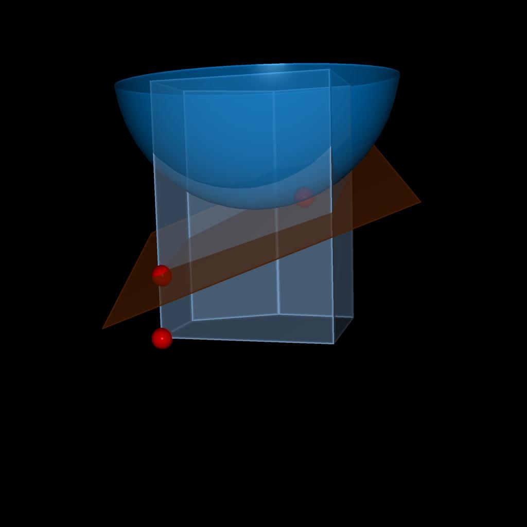
11 Geometry Interpretation min f(x) x2d f(x) x D R d

12 Compare to Classical Gradient Descent Define the descent direction as follows y, f(x) < 0 (16) Frank Wolfe algorithm: always choose the best descent direction over the entire domain D Classical gradient descent: x (k+1) = x (k) + α f(x (k) ) (17) where α 0 is the step size. It only uses local information to determine the step-directions. It faces the risk of walking out of the domain D. It requires projection steps after each iteration.

13 Greedy on a Convex Set 22 Convex Optimization without Projection Steps Algorithm 1 Greedy on a Convex Set Input: Convex function f, convex set D, target accuracy ε Output: ε-approximate solution for problem (2.1) Pick an arbitrary starting point x (0) D for k = 0... do Let α := 2 k+2 Compute s := ExactLinear ( f(x (k) ), D ) {Solve the linearized primitive problem exactly} or Compute s := ApproxLinear ( ) f(x (k) ), D, αc f {Approximate the linearized primitive problem} Update x (k+1) := x (k) + α(s x (k) ) end for We call a point x X an ɛ-approximation if g(x, d x ) ɛ for some choice of subgradient d x f(x).

14 Linearized Optimization Primitive In the above algorithm, ExactLinear(c, D) minimizes the linear function x, c over D. It returns s by s = arg min y, c (18) y D We search for a point s that realizes the current duality gap g(x), that is the distance to the linear approximation, as follows g(x, d x ) = f(x) w(x, d x ) = max y D x y, d x. (19)

15 Linearized Optimization Primitive In the above algorithm, ApproxLinear(c, D, ɛ ) approximates the minimum of the linear function x, c over D. It returns s such that s, c = arg min y, c + ɛ. (20) y D For several applications, this can be done significantly more efficiently than the exact variant.

16 The Curvature The Curvature constant C f of a convex and differentiable function f, with respect to a compact domain D is defined as C f = sup x,s D α [0,1] y=x+α(s x) 1 (f(y) f(x) y x, f(x) ) (21) α2 It bounds the gap between f(y) and its linearization. f(y) f(x) y x, f(x) is known as the Bregman divergence. For linear functions f, it holds that C f = 0.

17 Convergence in Primal Error Theorem 1 (Primal Convergence) For each k 1, the iterative x (k) of the exact variant of Algorithm 1 satisfies f(x (k) ) f(x ) 4C f K + 2, (22) where x ( ) D is an optimal solution to problem (1). For the approximate variant of Algorithm 1, it holds that f(x (k) ) f(x ) 8C f K + 2. (23) In other words, both algorithm variants deliver a solution of primal error at most ɛ after O( 1 ɛ ) many iterations.

18 Duality Gap Theorem 2 (Primal-Dual Convergence) Let K = 4Cf ɛ. We run the exact variant of Algorithm 1 for K iterations (recall that the step-sizes are given by α (k) = 2 k+2, 0 k K), and then continue for another K + 1 iterations, now with the fixed step-size α (k) = 2 K+2 for K k 2K + 1. Then the algorithm has an iterate x (ˆk), K ˆk 2K + 1, with duality gap bounded by g(x (ˆk) ) ɛ (24) The same statement holds for the approximate variant of Algorithm 1, when setting K = instead. 8Cf ɛ

19 Choose Step-Size by Line-Search Instead of the fixed step-size α = 2 α [0, 1] by line-search. If we define ( f α = f The optimal α is α = arg min f α [0,1] x (k+1) (α) ) = f k+2 ( α f α = s x (k), f, we can find the optimal ( ) x (k) + α(s x (k) ). (25) ( ) x (k) + α(s x (k) ). (26) x (k+1) (α) ) = 0. (27)

20 Greedy on a Convex Set using Line-Search A Projection-Free First-Order Method for Convex Optimization 29 Algorithm 2 Greedy on a Convex Set, using Line-Search Input: Convex function f, convex set D, target accuracy ε Output: ε-approximate solution for problem (3.1) Pick an arbitrary starting point x (0) D for k = 0... do Compute s := ExactLinear ( f(x (k) ), D ) or ( Compute s := ApproxLinear Find the optimal step-size α := arg min α [0,1] Update x (k+1) := x (k) + α(s x (k) ) end for ) f(x (k) ), D, 2Cf f k+2 ( x (k) + α(s x (k) ) ) If this equation can be solved for α, then the optimal such α can directly be used as the step-size in Algorithm 1, and the convergence guarantee of Theorem 2.3 still holds. This is because the improvement in each step will

21 Relating the Curvation to the Hessian Matrix Hessian matrix of f: is the second derivative of f, i.e. 2 f. Second order Taylor-expansion of function f at point x is f(x + α(s x)) =f(x) + α(s x) T f(x) where z [x, y] D and Thus, we have + α2 2 (s x)t 2 f(z)(s x) (28) y = x + α(s x) (29) α(s x) = y x, (30) f(y) = f(x) + (y x) T f(x) (y x)t 2 f(z)(y x) (31)

22 Relating the Curvation to the Hessian Matrix f(y) f(x) y x, f(x) = 1 2 (y x)t 2 f(z)(y x) (32) According to the definition of C f C f = sup x,s D α [0,1] y=x+α(s x) 1 (f(y) f(x) y x, f(x) ), (33) α2 we have C f 1 sup x,y D 2 (y x)t 2 f(z)(y x) (34) z [x,y] D

23 Relating the Curvation to the Hessian Matrix Lemma 2 For any twice differentiable convex function f over a compact convex domain D, it holds that C f 1 2 diam(d)2 sup λ max ( 2 f(z)) (35) z D where diam( ) is the Euclidean diameter of the domain.

24 Relatinig the Curvation to the Hessian Matrix Proof. According to Cauchy-Schwarz inequality we have a, b a b (36) (y x) T 2 f(z)(y x) y x 2 2 f(z)(y x) 2 (37) y x 2 2 f(z)(y x) 2 2 (38) y x 2 y x f(z) spec (39) diam(d) 2 sup λ max ( 2 f(z)) (40) z D Aa where A spec = sup 2 a 0 a 2 is the spectral norm, which is the largest eigenvalue for a positive-semidefinite A.

25 VS. Lipschitz-Continuous Gradient Lemma 3 Let f be a convex and twice differential function, and assume that the gradient f is Lipschitz-continuous over the domain D with Lipschitz-constant L > 0. Then C f 1 2 diam(d)2 L (41) where Lipschitz-continuous means there exits L > 0 satisfies f(y) f(x) 2 L y x 2 (42)

26 Figure 2.2 Some simple convex and nonconvex sets. Left. The hexagon, Optimizing whichover includes its boundary Convex (shown darker), Hulls is convex. Middle. The kidney shaped set is not convex, since the line segment between the two points in the set shown as dots is not contained in the set. Right. The square contains some boundary points but not others, and is not convex. Figure 2.3 The convex hulls of two sets in R 2. Left. The convex hull of a set of fifteen points (shown as dots) is the pentagon (shown shaded). Right. The convex hull of the kidney shaped set in figure 2.2 is the shaded set. The convex hull of a set V, denoted conv(v ), is the set of all convex combination of points in V : { conv(v ) = θ 1 x θ k x k x i V, θ i 0, i = 1,, k, Roughly speaking, a set is convex if every point in the set can be seen by every other point, along an unobstructed straight path between them, where unobstructed means lying in the set. Every affine set is also convex, since it contains the entire line between any two distinct points in it, and therefore also the line segment between the points. Figure 2.2 illustrates some simple convex and nonconvex sets in R 2. } We call a point of the form θ 1x 1 + θ kx k, where θ θ k = 1 and θ i 0, i = 1,..., k, aθconvex 1 + combination + θ k of the = points 1 x 1,..., x k. As with affine sets, it can be shown that a set is convex if and only if it contains every convex combination of its points. A convex combination of points can be thought of as a mixture or weighted average of the points, with θ i the fraction of x i in the mixture. The convex hull conv(v ) is always convex.. (43) The convex hull of a set C, denoted conv C, is the set of all convex combinations of points in C: It is the smallest convex set that contains V. conv C = {θ 1x θ kx k x i C, θ i 0, i = 1,..., k, θ θ k = 1}.

27 Optimizing over Convex Hulls Consider the case where domain D is the convex hull of a set V, i.e. D = conv(v ). Lemma 4 (Linear Optimization over Convex Hulls) Let D = conv(v ) for any subset V X, and D compact. Then any linear function y y, c will attain its minimum and maximum over D at some vertex v V. In many applications, the set V is often much easier to describe than the full compact domain D, the result in the above lemma will be usefull to solve the linearized subproblem ExactLinear() more efficiently.

28 Outline 1. Theoretical Results 2. Applications

29 many gradient evaluations. We will crucially make use of the fact t every linear function attains its minimum at a vertex of the simplex Sparse Approximation (SA) over the Simplex Formally, for any vector c R n, it holds that min s T c = min c i. T s n i The unit property Simplex is defined easy to verify as in the special case here, but is also a di consequence of the small Lemma 2.8 which we have proven for gen convex hulls, n = if {x we accept R n xthat 0, the x unit 1 = simplex 1} is the convex (44) hull of unit basis vectors. We have obtained that the internal linearized primi Then, optimization can be solved onexactly Simplex byischoosing ExactLinear min (c, f(x) n ) := e i with i = arg min (45) c i. x n i Algorithm 3 Sparse Greedy on the Simplex Input: Convex function f, target accuracy ε Output: ε-approximate solution for problem (3.1) Set x (0) := e 1 for k = 0... do Compute i := arg min i ( f(x (k) ) ) i Let α := 2 k+2 Update x (k+1) := x (k) + α(e i x (k) ) end for

30 SA over the Simplex Theorem 3 (Convergence of Sparse Greedy on the Simplex) For each k 1, the iterate x (k) of the above algorithm satisfies f(x k ) f(x ) 4C f k + 2 (46) where x n is an optimal solution to problem in (45). Furthermore, for any ɛ > 0, after at most 2 4Cf ɛ + 1 = O( 1 ɛ ) many steps, it has an iterate x (k) of sparsity O( 1 ɛ ), satisfying g(x (k) ) ɛ.

31 SA over the Simplex Its duality gap is g(x, d x ) = f(x) w(x, d x ) (47) ( ) = f(x) min f(x) + y x, d x (48) y D = max y D x y, d x (49) = x T d x min y D yt d x (50)

32 Figure 2.2 Some simple convex and nonconvex sets. Left. The hexagon, SA over the which includes Simplex its boundary (shown darker), is convex. Middle. The kidney shaped set is not convex, since the line segment between the two points in the set shown as dots is not contained in the set. Right. The square contains some boundary points but not others, and is not convex. Figure 2.3 The convex hulls of two sets in R 2. Left. The convex hull of a set of fifteen points (shown as dots) is the pentagon (shown shaded). Right. The convex hull of the kidney shaped set in figure 2.2 is the shaded set. The convex hull of a set V, denoted conv(v ), is the set of all convex combination of points in V : { conv(v ) = θ 1 x θ k x k x i V, θ i 0, i = 1,, k, Roughly speaking, a set is convex if every point in the set can be seen by every other point, along an unobstructed straight path between them, where unobstructed means lying in the set. Every affine set is also convex, since it contains the entire line between any two distinct points in it, and therefore also the line segment between the points. Figure 2.2 illustrates some simple convex and nonconvex sets in R 2. } We call a point of the form θ 1x 1 + θ kx k, where θ θ k = 1 and θ i 0, i = 1,..., k, aθconvex 1 + combination + θ k of the = points 1 x 1,..., x k. As with affine sets, it can be shown that a set is convex if and only if it contains every convex combination of its points. A convex combination of points can be thought of as a mixture or weighted average of the points, with θ i the fraction of x i in the mixture. The convex hull conv(v ) is always convex.. (51) The convex hull of a set C, denoted conv C, is the set of all convex combinations of points in C: It is the smallest convex set that contains V. conv C = {θ 1x θ kx k x i C, θ i 0, i = 1,..., k, θ θ k = 1}.

33 SA over the Simplex Lemma 5 (Linear Optimization over Convex Hulls) Let D = conv(v ) for any subset V X, and D compact. Then any linear function y y, c will attain its minimum and maximum over D at some vertex v V. Proof. 1 Assume s D satisfies s, c = max y D y, c. 2 Represent s = i α iv i, where i α i = 1. 3 We have s, c = α i v i, c = α i v i, c (52) i i

34 SA over the Simplex Its duality gap is g(x, d x ) = f(x) w(x, d x ) (53) ( ) = f(x) min f(x) + y x, d x (54) y D Because, here we have then = max y D x y, d x (55) = x T d x min y D yt d x (56) D = n = {x R n x 0, x 1 = 1} (57) g(x) = g(x, f(x)) = x T f(x) min i ( f(x)) i (58)

35 SA over the Simplex: Example Consider the following problem min x n f(x) = x 2 2 = x T x, (59) whose gradient is f(x) = 2x. Then, we have f(y) f(x) y x, f(x) = y T y x T x 2(y x) T x (60) According to the definition of C f C f = sup x,s D α [0,1] y=x+α(s x) = y x 2 2 (61) = x + α(s x) x 2 2 (62) = α 2 s x 2 2 (63) 1 (f(y) f(x) y x, f(x) ) (64) α2 = sup x,s n x s 2 2 = diam( n ) 2 = 2 (65)

36 SA with Bounded l 1 -Norm The l 1 -ball is defined as n = {x R n x 1 1}. (66) Then, optimization with bounded l 1 -norm is Observation 2 For any vector c R n, it holds that where i arg max j c j. min x n f(x) (67) e i sgn(c i ) arg max y T c (68) y n

37 Observe that in each iteration, this algorithm only introd one new non-zero coordinate, so that the sparsity of x (k) is SAUsing withthis Bounded observation l 1 -Norm for c = f(x) in our general Alg therefore directly obtain the following simple method for l convex optimization, as depicted in the Algorithm 4. Algorithm 4 Sparse Greedy on the l 1 -Ball Input: Convex function f, target accuracy ε Output: ε-approximate solution for problem (3.3) Set x (0) := 0 for k = 0... do ( Compute i := arg max i f(x (k) ), i and let s := e i sign (( f(x (k) ) ) ) i Let α := 2 k+2 Update x (k+1) := x (k) + α(s x (k) ) end for

38 SA with Bounded l 1 -Norm Theorem 4 (Convergence of Sparse Greedy on the l 1 -Ball) For each k 1, the iterate x (k) of the above algorithm satisfies f(x k ) f(x ) 4C f k + 2 (69) where x n is an optimal solution to problem in (67). Furthermore, for any ɛ > 0, after at most 2 4Cf ɛ + 1 = O( 1 ɛ ) many steps, it has an iterate x (k) of sparsity O( 1 ɛ ), satisfying g(x (k) ) ɛ.

39 Optimization with Bounded l -Norm The l -ball is defined as n = {x R n x 1}. (70) Then, optimization with bounded l 1 -norm is Observation 3 For any vector c R n, it holds that where (s c ) i = sgn(c i ) { 1, 1}. min f(x) (71) x n s c arg max y T c (72) y n

40 Optimization with Bounded l -Norm Optimization with Bounded l -Norm Algorithm 5 Sparse Greedy on the Cube Input: Convex function f, target accuracy ε Output: ε-approximate solution for problem (3.4) Set x (0) := 0 for k = 0... do Compute the sign-vector s of f(x (k) ), such that s i = sign (( f(x (k) ) ) i), i = 1..n Let α := 2 k+2 Update x (k+1) := x (k) + α(s x (k) ) end for Theorem 3.7. For each k 1, the iterate x (k) of Algorithm 5

41 Optimization with Bounded l -Norm Theorem 5 (Convergence of Sparse Greedy on the l 1 -Ball) For each k 1, the iterate x (k) of the above algorithm satisfies f(x k ) f(x ) 4C f k + 2 (73) where x n is an optimal solution to problem in (71). Furthermore, for any ɛ > 0, after at most 2 4Cf ɛ many steps, it has an iterate x (k) with g(x (k) ) ɛ. + 1 = O( 1 ɛ )

42 Semidefinite Optimization (SDO) with Bounded Trace The set of positive semidefinite (PSD) matrices of unit trace is defined as S = {X R n n X 0, Tr(X) = 1}. (74) Then, optimization of PSD with bounded trace is min f(x) (75) x S

43 52 Applications to Sparse and Low Rank Approximation SDO with Bounded Trace trix M S n n. We will see that in practice for example Lanczos or the power method can be used as the internal optimizer ApproxLinear(). Algorithm 6 Hazan s Algorithm / Sparse Greedy for Bounded Trace Input: Convex function f with curvature C f, target accuracy ε Output: ε-approximate solution for problem (3.5) Set X (0) := vv T for an arbitrary unit length vector v R n. for k = 0... do Let α := 2 k+2 Compute v := v (k) = ApproxEV ( f(x (k) ), αc f ) Update X (k+1) := X (k) + α(vv T X (k) ) end for Here ApproxEV(A, ε ) is a subroutine that delivers an approximate ApproxEV(A, ɛ ) returns v, which satisfies smallest eigenvector (the eigenvector corresponding to the smallest eigenvalue) to a matrix A with the desired accuracy ε > 0. More precisely, it v T Av λ min (A) + ɛ must return a unit length vector v such that v T (76) Av λ min (A) + ε. Note that as our convex function f takes a symmetric matrix X as an argument, its gradients f(x) are given as symmetric matrices as well.

44 SDO with Bounded Trace Theorem 6 For each k 1, the iterate X (k) of the above algorithm satisfies f(x k ) f(x ) 8C f k + 2 (77) where X S is an optimal solution to problem in (75). Furthermore, for any ɛ > 0, after at most 2 8Cf ɛ + 1 = O( 1 ɛ ) many steps, it has an iterate X (k) of rank O ( 1 ɛ ), satisfying g(x (k) ) ɛ.

45 Nuclear Norm Regularization We consider the following problem which is equivalent to min f(z) + µ Z (78) Z R m n min f(z) (79) Z R m n, Z t 2 where f(z) is any differentiable convex function. is the nuclear norm (trace norm, Schatten 1-norm, the Ky Fan r-norm) of a matrix Z = r σ i (Z) (80) i=1 where σ i is the i-th largest singular value of Z, r is the rank of Z

46 Nuclear Norm Low Rank Frobenius norm: Z F = Z, Z = Tr(Z T Z) 1 2 ( m n r = = i=1 j=1 X 2 ij i=1 σ 2 i ) 1 2 (81) Operator norm (induced 2-norm): Z = λ max (Z T Z) = σ 1 (Z) (82) Nuclear norm: Z = r σ i (Z) (83) i=1

47 Nuclear Norm Low Rank According to the definitions of Z F = ( r i=1 σ 2 i we have following inequalities ) 1 2, Z = σ 1 (Z), Z = r σ i (Z), i=1 Z Z F Z r Z F r Z (84)

48 Nuclear Norm Low Rank C is a given convex set. The convex envelop of a (possible nonconvex) function f : C R is the largest convex function g such that g(z) f(z) for all z C. g is the best pointwise approximation to f. According to the above inequalities, if Z 1, we have rank(z) Z Z = rank(z) Z (85) Nuclear norm is the tightest convex lower bound of the rank function. Theorem 7 The convex envelop of rank(z) on the set {Z R m n : Z 1} is the nuclear norm Z.

49 Corollary 1 Any nuclear norm regularized problem min f(z) (86) Z R m n, Z t 2 is equivalent to a bounded trace convex problem min ˆf(X) X S (m+n) (m+n) s. t. Tr(X) = t X 0 (87) where ˆf is defined by ˆf(X) = f(z) and ( V Z X = Z T W where V S m m, W S n n. ) (88)

50 function argument X needs to be rescaled by 1 t in order to have unit trace, which however is a very simple operation in practical applications. Therefore, we can directly apply Hazan s Algorithm 6 for any max-norm regularized problem as follows: Nuclear Norm Regularization Algorithm 8 Nuclear Norm Regularized Solver Input: A convex nuclear norm regularized problem (4.2), target accuracy ε Output: ε-approximate solution for problem (4.2) 1. Consider the transformed symmetric problem for ˆf, as given by Corollary Adjust the function ˆf so that it first rescales its argument by t 3. Run Hazan s Algorithm 6 for ˆf(X) over the domain X S. Using our analysis of Algorithm 6 from Section 3.4.1, we see that Algorithm 8 runs in time near linear in the number N f of non-zero entries of the min f(x) gradient f. This makes it very attractive in min particular for ˆf(X) X S (n) (n) X S (m+n) (m+n) recommender systems applications and matrix completion, where f is a sparse matrix (same sparsity s. t. Tr(X) pattern= as 1, the observed entries), which s. t. we Tr(X) will = discuss t, in more detail in XSection (89) X 0 (90)

51 Nuclear Norm Regularization Corollary 2 After at most O ( ) 1 ɛ many iterations, Algorithm 8 obtains a solution that is ɛ close to the optimum of (86). The algorithm requires a total of Õ probability). ( Nf ɛ 1.5 ) arithmetic operations (with high

52 Thank You!