Motion estimation. Lihi Zelnik-Manor

Transcription

1 Motion estimation Lihi Zelnik-Manor

2 Optical Flow Where did each piel in image 1 go to in image 2

3 Optical Flow Pierre Kornprobst's Demo

4 ntroduction Given a video sequence with camera/objects moving we can better understand the scene if we find the motions of the camera/objects.

5 Scene nterpretation How is the camera moving? How man moving objects are there? Which directions are the moving in? How fast are the moving? Can we recognize their tpe of motion (e.g. walking, running, etc.)?

6 Applications Recover camera ego-motion. Result b MobilEe (

7 Applications Motion segmentation Result b: L.Zelnik-Manor, M.Machline, M.rani Multi-bod Segmentation: Revisiting Motion Consistenc To appear, JCV

8 Applications Structure from Motion nput Reconstructed shape Result b: L. Zhang, B. Curless, A. Hertzmann, S.M. Seitz Shape and motion under varing illumination: Unifing structure from motion, photometric stereo, and multi-view stereo CCV 03

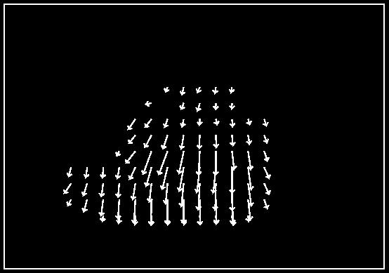
9 Eamples of Motion fields Forward motion Rotation Horizontal translation Closer objects appear to move faster!!

10 Motion Field & Optical Flow Field Motion Field = Real world 3D motion Optical Flow Field = Projection of the motion field onto the 2d image CCD 3D motion vector 2D optical flow vector u= u,v ( )

11 When does it break? The screen is stationar et displas motion Homogeneous objects generate zero optical flow. Fied sphere. Changing light source. Non-rigid teture motion

12 The Optical Flow Field Still, in man cases it does work. Goal: Find for each piel a velocit vector which sas: How quickl is the piel moving across the image n which direction it is moving u= ( u,v)

13 How do we actuall do that?

14 Estimating Optical Flow Assume the image intensit is constant Time = t Time = tdt (, ) d, d ( ), = (, t) ( d, d, t dt)

15 Brightness Constanc Equation,, t = d, d, t dt ( ) ( ) First order Talor Epansion Simplif notations: Divide b dt and denote: =, t (, t) d d dt d d dt u= u d dt v= v = t d dt = 0 t Gradient and flow are orthogonal Problem : One equation, two unknowns

16 Problem : The Aperture Problem For points on a line of fied intensit we can onl recover the normal flow Time t Time tdt? Where did the blue point move to? We need additional constraints

17 Use Local nformation Sometimes enlarging the aperture can help

18 Local smoothness Lucas Kanade (1984) Assume constant (u,v) in small neighborhood t v u = [ ] t v u = = t t v u A = b u

19 Lucas Kanade (1984) Goal: Minimize Au b 2 Method: Least-Squares A u = b A T A u = A T b 21 u = ( T ) 1 T A A A b

20 How does Lucas-Kanade behave? = 2 2 T A A We want this matri to be invertible. i.e., no zero eigenvalues ( ) b A A A T T 1 u =

21 How does Lucas-Kanade behave? Edge A T A becomes singular (, ) (, ) 2 2 = 0 0 is eigenvector with eigenvalue 0

22 How does Lucas-Kanade behave? Homogeneous ( ) 0, A T A 0 0 eigenvalues

23 How does Lucas-Kanade behave? Tetured regions two high eigenvalues ( ) 0,

24 How does Lucas-Kanade behave? Edge A T A becomes singular Homogeneous regions low gradients High teture A T A 0

25 terative Refinement Estimate velocit at each piel using one iteration of Lucas and Kanade estimation u = Warp one image toward the other using the estimated flow field (easier said than done) ( T ) 1 T A A A b Refine estimate b repeating the process

26 Optical Flow: terative Estimation estimate update û nitial guess: Estimate: u 0 = 0 1= ˆ 0 u u u 0

27 Optical Flow: terative Estimation f ( u ) 1 1 estimate update û nitial guess: Estimate: u 1 u ˆ 2 = u1 u 0

28 Optical Flow: terative Estimation f ( u ) 1 2 estimate update û nitial guess: Estimate: u 2 3 = ˆ 2 u u u 0

29 Optical Flow: terative Estimation f ( u ) f ( )

30 Optical Flow: terative Estimation Some mplementation ssues: Warping is not eas (ensure that errors in warping are smaller than the estimate refinement) Warp one image, take derivatives of the other so ou don t need to re-compute the gradient after each iteration. Often useful to low-pass filter the images before motion estimation (for better derivative estimation, and linear approimations to image intensit)

31 Other break-downs Brightness constanc is not satisfied Correlation based methods A point does not move like its neighbors what is the ideal window size? Regularization based methods The motion is not small (Talor epansion doesn t hold) Aliasing Use multi-scale estimation

32 Optical Flow: Aliasing Temporal aliasing causes ambiguities in optical flow because images can have man piels with the same intensit..e., how do we know which correspondence is correct? actual shift estimated shift nearest match is correct (no aliasing) To overcome aliasing: coarse-to to-fine estimation. nearest match is incorrect (aliasing)

33 Multi-Scale Flow Estimation u=1.25 piels u=2.5 piels u=5 piels image t-1 u=10 piels image t1 Gaussian pramid of image t Gaussian pramid of image t1

34 Multi-Scale Flow Estimation run Lucas-Kanade warp & upsample run Lucas-Kanade... image t-1 image t1 Gaussian pramid of image t Gaussian pramid of image t1

35 Eamples: Motion Based Segmentation nput Segmentation result Result b: L.Zelnik-Manor, M.Machline, M.rani Multi-bod Segmentation: Revisiting Motion Consistenc To appear, JCV

36 Eamples: Motion Based Segmentation nput Segmentation result Result b: L.Zelnik-Manor, M.Machline, M.rani Multi-bod Segmentation: Revisiting Motion Consistenc To appear, JCV

37 Other break-downs Brightness constanc is not satisfied Correlation based methods A point does not move like its neighbors what is the ideal window size? Regularization based methods The motion is not small (Talor epansion doesn t hold) Aliasing Use multi-scale estimation

38 Robust Estimation Sources of outliers (multiple motions): specularities / highlights jpeg artifacts / interlacing / motion blur multiple motions (occlusion boundaries, transparenc) Noise distributions are often non-gaussian, having much heavier tails. Noise samples from the tails are called outliers.

39 Regularization Horn and Schunk (1981) Add global smoothness term Smoothness error: Error in brightness constanc equation E E ( 2 2) ( 2 2 u u v v ) dd s = D ( ) 2 u v dd c = D t Minimize: E λ c E s Solve b calculus of variations

40 Robust Estimation Black & Anandan (1993) Regularization can over-smooth across edges Use smarter regularization

41 Least Squares Estimation Standard Least Squares Estimation allows too much influence for outling points ) ( ) ) ( ) ( ) ( ) ( 2 m m m E i i i i i = = = = ρ ψ ρ ρ ( nfluence

42 Robust Estimation Problem: Least-squares estimators penalize deviations between data & model with quadratic error f n (etremel sensitive to outliers) error penalt function influence function Redescending error functions (e.g., Geman-McClure) help to reduce the influence of outling measurements. error penalt function influence function

43 Robust Estimation Black & Anandan (1993) Regularization can over-smooth across edges Use smarter regularization Minimize: D ( u v ) λ[ ρ ( u u ) ( v v )] dd 1 t 2, ρ2, ρ Brightness constanc Smoothness

44 Eamples: Motion Based Segmentation nput Segmentation result Optical Flow estimation b: M. J. Black and P. Anandan, A framework for the robust estimation of optical flow, CCV 93 Segmentation b: L.Zelnik-Manor, M.Machline, M.rani Multi-bod Segmentation: Revisiting Motion Consistenc, JCV 06

45 Parametric motion estimation

46 Global (parametric) motion models 2D Models: Affine Quadratic Planar projective transform (Homograph) 3D Models: nstantaneous camera motion models Homographepipole PlaneParalla

47 Motion models Translation Affine Perspective 3D rotation 2 unknowns 6 unknowns 8 unknowns 3 unknowns

48 Affine Motion For panning camera or planar surfaces: p p p v p p p u = = t p p p p p p = ) ( ) ( [ ] t = p Onl 6 parameters to solve for Better results Least Square Minimization (over all piels): [ ] 2 = a Err ) ( [ ] t p

49 Quadratic instantaneous approimation to planar motion Other 2D Motion Models q q q q q v q q q q q u = = v u h h h h h h h h h h h h = = = = ', ' and ' ' Projective eact planar motion

50 3D Motion Models Z T T v Z T T u Z Y Z Y X Z X Z Y X ) ( ) (1 ) ( ) (1 2 2 Ω Ω Ω = Ω Ω Ω = v u t h h h t h h h t h h h t h h h = = = = ', ' : and ' ' γ γ γ γ ) ( 1 ) ( t t t v t t t u w w = = = = γ γ γ γ Local Parameter: Z Y X Z Y X T T T,,,,, Ω Ω Ω ), ( Z nstantaneous camera motion: Global parameters: Global parameters: ,,,,, t t t h h ), ( γ HomographEpipole Local Parameter: Residual Planar Paralla Motion Global parameters: 3 2 1,, t t t ), ( γ Local Parameter:

51 Segmentation of Affine Motion = nput Segmentation result Result b: L.Zelnik-Manor, M.rani Multi-frame estimation of planar motion, PAM 2000

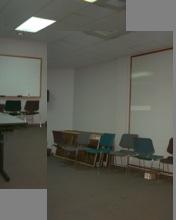
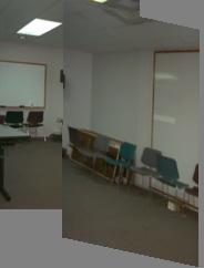
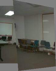
52 Panoramas nput Motion estimation b Andrew Zisserman s group

53 Stabilization Result b: L.Zelnik-Manor, M.rani Multi-frame estimation of planar motion, PAM 2000

54 Sparse matching

55 Patch matching (revisited) How do we determine correspondences? block matching or SSD (sum squared differences)

56 Correlation and SSD For larger displacements, do template matching Define a small area around a piel as the template Match the template against each piel within a search area in net image. Use a match measure such as correlation, normalized correlation, or sum-of-squares difference Choose the maimum (or minimum) as the match Sub-piel estimate (Lucas-Kanade)

57 Discrete Search vs. Gradient Based Consider image translated b 2 1, 0 0 2, 1 )), ( ), ( ), ( ( )), ( ), ( ( ), ( v v u u v u v u E η = = u 0,v 0 ), ( ), ( ), ( ), ( ), ( v u η = = The discrete search method simpl searches for the best estimate. The gradient method linearizes the intensit function and solves for the estimate

58 Tracking result

59 Laered Scene Representations

60 Motion representations How can we describe this scene?

61 Block-based motion prediction Break image up into square blocks Estimate translation for each block Use this to predict net frame, code difference (MPEG-2)

62 Laered motion Break image sequence up into laers : = Describe each laer s motion

63 Laered Representation For scenes with multiple affine motions Estimate dominant motion parameters Reject piels which do not fit Convergence Restart on remaining piels

64 Some Results Nebojsa Jojic and Brendan Fre, "Learning Fleible Sprites in Video Laers, CVPR 2001.

65 A bit more fun Action Recognition

66 Recognizing Actions at a Distance A.A. Efros, A.C. Berg, G. Mori, J. Malik mage frame Optical flow F, Use optical flow as a template for frame classification

67 Recognizing Actions at a Distance A.A. Efros, A.C. Berg, G. Mori, J. Malik mage frame Optical flow F, F, F F, F, F, F blurred F, F, F, F

68 Recognizing Actions at a Distance A.A. Efros, A.C. Berg, G. Mori, J. Malik Database: Test sequence: For each frame in test sequence find closest frame in database

69 Recognizing Actions at a Distance A.A. Efros, A.C. Berg, G. Mori, J. Malik Red bars show classification results

70 Recognizing Actions at a Distance A.A. Efros, A.C. Berg, G. Mori, J. Malik View Greg n World Cup video

71 References on Optical Flow Lucas-Kanade method: B.D. Lucas and T. Kanade An terative mage Registration Technique with an Application to Stereo Vision JCA '81 pp S. Baker and. Matthews Lucas-Kanade 20 Years On: A Unifing Framework JCV, Vol. 56, No. 3, March, 2004, pp (papers code) Regularization based methods: B. K. P. Horn and B. Schunck, "Determining Optical Flow," Artificial ntelligence, 17 (1981), pp Black, M. J. and Anandan, P., A framework for the robust estimation of optical flow, CCV 93, Ma, 1993, pp (papers code) Comparison of various optical flow techniques: Barron, J.L., Fleet, D.J., and Beauchemin, S. Performance of optical flow techniques. JCV, 1994, 12(1):43-77 Laered representation (affine): James R. Bergen P. Anandan Keith J. Hanna Rajesh Hingorani Hierarchical Model- Based Motion Estimation ECCV 92, pp

72 That s all for toda

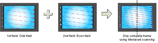
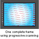
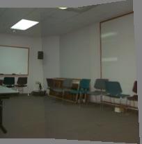
73 nterlace vs. progressive scan

74 Progressive scan

75 nterlace

76 Progressive scan vs. intelaced sensors Most camcorders are interlaced several eceptions (check the specs before ou bu!) some can be switched between progressive and interlaced Used to be true also for video cameras (interlaced) But now it s becoming the opposite man/most digital video cameras are progressive scan