Advanced Professional Training

Transcription

1 Advanced Professional Training Non Linea rand Stability

2 All information in this document is subject to modification without prior notice. No part of this manual may be reproduced, stored in a database or retrieval system or published, in any form or in any way, electronically, mechanically, by print, photo print, microfilm or any other means without prior written permission from the publisher. SCIA is not responsible for any direct or indirect damage because of imperfections in the documentation and/or the software. Copyright 2015 SCIA nv. All rights reserved. 2

3 Table of contents Table of contents Table of contents... 3 Introduction Professional training Introduction to non linear and stability... 1 Non-Linear behaviour of Structures Type of Non Linearity Non Linear Combinations... 2 Geometrical Non-Linearity also possible with Concept edition Overview Alpha critical Imperfections Global frame imperfection Initial bow imperfection e Example Global + Bow imperfection The second order calculation Timoshenko Newton-Raphson Physical Non-Linearity Plastic Hinges for Steel Structures Physical Non-Linear analysis for Concrete Structures General Plastic analysis von Mises yield criterion Finite element model Material properties General plasticity in SCIA Engineer Local Non-Linearity Beam Local Nonlinearity also available in the concept edition Members defined as Pressure only / Tension only Members with Limit Force Members with gaps Beam Local Nonlinearity including Initial Stress Members with Initial Stress Cable Elements Not available in the Professional edition Non-Linear Member Connections Support Nonlinearity Tension only / Pressure only Supports Nonlinear Springs for Supports Friction Supports D Elements D Membrane Elements Not in Professional Edition Pressure only Stability Calculations Stability Combinations Linear Stability Non-Linear Stability Troubleshooting Singularity Convergence References

4

5 Introduction 1.1. Professional training This course will explain the non linear and stability calculations in SCIA Engineer. Most of the modules necessary for this calculation are included in the Professional edition. For some options a concept edition is sufficient or for other options an expert edition or an extra module is required. This will always be indicated in the corresponding paragraph Introduction to non linear and stability In general, when modelling structures, a linear approach is followed. It can however be that certain parts of the structure do not behave linearly. Examples include supports or members which only act in compression or tension. This is where non-linear analysis is required. Another example is when performing structural analysis following the latest codes (i.e. Eurocode 3). When performing manual calculations, in most cases a linear 1st Order analysis is carried out. However, the assumptions of such analysis are not always valid and the codes then advise the use of 2 nd Order analysis, imperfections, etc. SCIA Engineer contains specialized modules covering non-linear and stability related issues. In this course, the different aspects of these modules are regarded in detail. In the first part of the course, the non-linear modules are looked upon. First the 2 nd Order calculation methods are explained and integrated with Eurocode 3. Next the local nonlinearities are examined including tension-only members, pressure-only supports, cable analysis, friction supports, etc. The non-linear part of the course is finished with an insight on how to apply imperfections according to Eurocode 3 using SCIA Engineer. The second part of the course examines Stability calculations: the determination of the elastic critical buckling load of a structure. This analysis can be used to calculate the buckling length of a part of the structure or to determine if a 1 st Order analysis may be carried out. The final chapter provides some common failure messages which occur during a non-linear analysis. This chapter points out the most likely causes of singularities and convergence failures. 1

6 Non-Linear behaviour of Structures 2.1. Type of Non Linearity The non-linear behaviour of structures can be categorised in three different groups: - Geometrical non-linearity: The displacements are dependent on the strains in a non-linear way. - Physical non-linearity: The stresses are dependent on the strains in a non-linear way. - Local non-linearity: The geometry or the boundary conditions of the structure change during the solving of the equations. These three types of non linearities will be examined in detail in the following chapters. For a complete overview and theoretical background, reference is made to [1], [2], [3], [4], [5] and [6]. To be able to use non linearities in SCIA Engineer this functionality should be enables in the Project data dialogue: And in the right column the necessary nonlinearity should be activated Non Linear Combinations During a linear analysis, the principle of superposition is valid: the load cases are calculated and the combinations are composed after the calculation. For a non-linear analysis, this principle is not valid anymore. The combinations have to be assembled before starting the calculation. In SCIA Engineer, this is done by defining Nonlinear Combinations. A non-linear combination is defined as a list of load cases where each load case has a specified coefficient. 2

7 In addition, for each non-linear combination it is possible to specify an initial Bow Imperfection and/or a Global Imperfection. Imperfections are regarded in Chapter 6. Note - The combinations defined as linear combinations can be imported as non-linear combinations. It is however important to keep in mind that during a non-linear calculation no combinations are generated. This implies for example that code specific combinations must first be exploded to linear combinations. These linear combinations can then be imported as non-linear combinations. This method makes sure that the code coefficients and relations between the load cases are correctly taken into account for the non-linear calculation. - To view the extreme results for the non-linear calculation, the non-linear combinations can be grouped within a result class. - The amount of non-linear combinations is limited to

8 Geometrical Non-Linearity also possible with Concept edition The options described here for the geometrical non linearities are also possible with a Concept edition. So the Professional edition is not required for this chapter, except for the stability calculation (and the calculation of cr as explained shortly in this chapter). The non-linear behaviour is caused by the magnitude of the deformations. Take for example a simple beam: during a linear analysis, the relative deformation of the end nodes, in the direction of the beam axis is dependent on the strain of the beam. Due to a curvature of the beam, the distance between the end nodes is changed also. This implicates that the total strain is now not solely dependent on the displacement. This relation can now be looked upon for different cases: a) Small displacements, small rotations and small strains; b) Large displacements, Large rotations and small strains; c) Large displacements, Large rotations and Large strains; In SCIA Engineer, methods a) and b) have been implemented for the analysis of geometrical non-linear structures. Method c) is less common in structural applications (for example rubber). Method a) is called the Timoshenko method; method b) is called the Newton-Raphson method. To activate the Geometrical Non-Linearity, the functionality Nonlinearity > 2 nd Order Geometrical nonlinearity must be activated. 4

9 3.1. Overview Advanced Professional Training Non Linear and Stability Global analysis aims at determining the distribution of the internal forces and moments and the corresponding displacements in a structure subjected to a specified loading. The first important distinction that can be made between the methods of analysis is the one that separates elastic and plastic methods. Plastic analysis is subjected to some restrictions. Another important distinction is between the methods, which make allowance for, and those, which neglect the effects of the actual, displaced configuration of the structure. They are referred to respectively as second-order theory and first-order theory based methods. The second-order theory can be adopted in all cases, while first-order theory may be used only when the displacement effects on the structural behavior are negligible. The second-order effects are made up of a local or member second-order effects, referred to as the P- effect, and a global second-order effect, referred to as the P- effect. On the next page an overview of the global analysis following the EN , chapter 5, will be given: o o o o o All the rules in this overview are given in the EN art. 5. For each step the rule will be indicated. The first rule ( cr > 10) will be explained in EN art (3). In this overview 3 paths are defined: Path 1: In this path a first order calculation will be executed Path 2: In this path a second order calculation will be executed with global (and bow) imperfections. Path 3: In this path a second order calculation will be executed with the buckling shape of the construction as imperfection. The calculation will become more precise when choosing for a higher path. The lower paths will result in a faster calculation, because a first order calculation can be executed without iterations, but this first-order theory may be used only when the displacement effects on the structural behavior are negligible. In the next paragraphs the rules in this overview will be explained. To take into account all non-linearities in the model, non-linear load combinations are made. 5

10 Structural Frame Stability 5.2.1(3) cr 10 Yes No 5.2.2(3)b 5.2.2(3)a 5.3.2(11) Global Imperfection 5.3.2(6) cr (5) No N Ed > 25% N cr (member) Yes cr e 0 if required e 0 in all members 1a 1b 2a 2b 2c 3 1 st Order Analysis 2 nd Order Analysis Increase sway effects with: cr No Members with e 0 Yes 5.2.2(3)c l b based on a global buckling mode 5.2.2(7)b l b taken equal to L Stability Check in plane 5.2.2(7)a Stability Check out of plane + LTB Check Section Check With: cr Elastic critical buckling mode. L Member system length Buckling Length l b Path 1a specifies the so called Equivalent Column Method. In step 1b and 2a l b may be taken equal to L. This is according to EC-EN so the user does not have to calculate the buckling factor =1. In further analysis a buckling factor smaller than 1 may be justified. 6

11 3.2. Alpha critical Advanced Professional Training Non Linear and Stability The calculation of alpha critical is done by a stability calculation in SCIA Engineer. For this calculation a Professional or an Expert edition is necessary, so with the concept edition is this not possible. The stability calculation has been inputted in module esas.13. According to the EN , 1 st Order analysis may be used for a structure, if the increase of the relevant internal forces or moments or any other change of structural behaviour caused by deformations can be neglected. This condition may be assumed to be fulfilled, if the following criterion is satisfied: for elastic analysis With: α cr : the factor by which the design loading has to be increased to cause elastic instability in a global mode. F Ed : the design loading on the structure. F cr : the elastic critical buckling load for global instability, based on initial elastic stiffnesses. If α cr has a value lower then 10, a 2 nd Order calculation needs to be executed. Depending on the type of analysis, both Global and Local imperfections need to be considered. EN prescribes that 2 nd Order effects and imperfections may be accounted for both by the global analysis or partially by the global analysis and partially through individual stability checks of members. The calculation of Alpha critical and also Path 3 from the diagram of the previous paragraph will be explained in the chapter Stability. Example: Imperfections2D.esa The diagram is now illustrated on a steel frame including a global imperfection. This benchmark project is examined in detail in references [20] and [23]. A stability calculation for the frame gives a critical load factor α cr of 13,17 > 10 This indicates that 2 nd Order effects are negligible and a 1 st Order analysis may be used for the structure. Path 1a can thus be followed and a 1 st Order Calculation is executed. A Steel Code Check gives the following results: When Path 2a is followed, using a Global imperfection and a 2 nd Order Calculation according to Timoshenko, the Steel Code Check shows the following: 7

12 It can be seen that the results are practically the same which is as expected since the α cr is larger then 10. The input of imperfections and execution of a Stability Calculation will be regarded in detail further in this course Imperfections When performing a non-linear calculation, it is possible to input initial geometrical imperfections: initial deformations and curvatures. These imperfections take into account the fact that the structure is for example a bit inclined instead of perfectly vertical or that the members are not completely straight. To input geometrical imperfections, the functionality Nonlinearity > Initial deformations and curvature must be activated. For each non-linear combination, the imperfections can then be set. 8

13 Difference is made between Global imperfections (Initial deformations) and Bow Imperfections (Curvatures) Global frame imperfection The nodal coordinates define the geometry of the structure. Using initial deformations as global imperfections, additional displacements (in X and Y direction) can be inputted. These displacements will thus alter the geometry. The structure itself can therefore be modelled as straight; the inclination is given by the global imperfection. The global imperfection can be set in the following ways: - Simple Inclination - Deformation from Load case - Inclination Functions - Buckling Shape Simple Inclination The imperfection is defined as a simple inclination. The inclination is defined in mm per m height of the structure. More specifically a horizontal displacement is given in the global X and/or Y direction which has a linear relation to the height (global Z direction). Deformation from Load case The imperfection is defined by the displacements of a specified load case. This option can be used to take into account for example the imperfections due to the self-weight. Especially for slender beams this can be important. 9

14 Inclination Functions The imperfection is defined by a deformation-to-height curve, similar to the Simple Inclination. The curve can then be assigned to an appropriate non-linear combination. These inclination functions are entered through Main -> Library -> Structure, Analysis -> Initial deformations : When the type is set to Manual input, the function can be inputted by specifying the height and the horizontal displacement. The type Factor allows a factor to be inputted at each height. In the definition of a non-linear combination, a manually inputted function can then be multiplied by this factor function. 10

15 When choosing EN art (3), the inclination function is calculated according to the code. As shown during the 2 nd Order calculations, Eurocode 3 ref.[27] defines the global imperfection the following way: but With: h The height of the structure in meters m The number of columns in a row including only those columns which carry a vertical load N Ed not less than 50% of the average value of the vertical load per column in the plane considered. 11

16 These parameters can be inputted after which the imperfection is automatically calculated: An inclination function is defined independent of an axis. This means that the same function can be used to define the displacement in X in function of Z, or Y in function of Z, or X in function of Y, In the definition of a non-linear combination, it can be specified between which axes the function defines a relation. The Sense option allows the imperfection to be applied in the positive or negative direction (according to the chosen global direction). This way, a non-linear combination can for example be copied, where the original has a positive sense and the copy a negative sense to take into account both possibilities. Instead of the Sense, the Factor function can be applied as specified above. The values of the factor function will be multiplied with the values of the defined inclination function. 12

17 Buckling Shape As an alternative to Global and Local imperfections, paragraph 5.3.2(11) of Eurocode 3 Ref.[27] allows the use of a buckling shape as a unique imperfection. For this option the Professional or Expert edition is necessary. This option has been inputted in module esas.13. To input geometrical imperfections, the functionality Nonlinearity > Initial deformations and curvature and Stability must be activated. The calculation of the buckling shape through a stability calculation will be looked upon in Chapter 6. Since the buckling shape is dimensionless, Eurocode gives the formula to calculate the amplitude init of the imperfection. In Ref.[29] examples are given to illustrate this method. In this reference, the amplitude is given as follows: init N e0 E I cr '' y cr,max cr 1 M Rk e 0 0,2 for 0, 2 N Rk 1 2 M 1 2 With: N Rk N cr = The imperfection factor for the relevant buckling curve. = The reduction factor for the relevant buckling curve, depending on the relevant cross-section. N Rk = The characteristic resistance to normal force of the critical crosssection, i.e. N pl,rk. N cr = Elastic critical buckling load. M Rk = The characteristic moment resistance of the critical cross-section, i.e. M el,rk or M el,rk as relevant. cr = Shape of the elastic critical buckling mode. Maximal second derivative of the elastic critical buckling mode. '' cr,max 13

18 The value of init can then be entered in the field Max deformation. This procedure will be illustrated in further in this course in the Chapter 6 concerning Stability Initial bow imperfection e 0 During a linear calculation, the members are taken to be ideally straight. Using bow imperfections, a local curvature can be defined for each element. A normal force in a member will thus lead to additional moments. These additional moments shall only be taken into account for members with compressive forces. To obtain correct results using bow imperfections, it is required to refine the number of 1D mesh elements. The local imperfection can be set in the following ways: - Simple Curvature - According to Buckling Data SCIA Engineer will automatically apply the curvature in the following way, which is in most cases the de-favourable sense: After the first iteration step, the deflection in the middle determines the sign of the initial bow imperfection. If there is no deflection the alternating pattern is used and the beam will deform with a sinusoidal form through its nodes. Simple Curvature Using this option, a curvature can manually be inputted. This curvature will be used for all members in the project. This method is quite convenient when the same type of cross-section (buckling curve) is used throughout the project like for example scaffolds, framework, 14

19 According to Buckling Data A bow imperfection according to buckling data allows the user to specify different curvatures for each used buckling data. In the Buckling and relative lengths properties of a member, the bow imperfection can be set. As seen during the 2 nd Order calculations, Eurocode 3 Ref.[27] defines the initial bow imperfection using the following table: Where L is the member length. When the options EN Table 5.1 elastic/plastic are chosen, SCIA Engineer will check the buckling curve of the member and will apply the specified imperfection automatically on the member. This imperfection is always applied which corresponds to Path 2c of the diagram seen during the 2 nd Order calculations. The options EN Table 5.1 elastic/plastic if required will apply the imperfection only if the normal force N Ed in a member is higher than 25% of the member s critical buckling load N cr as specified in Eurocode. This corresponds to Path 2b of the diagram. 15

20 When selecting Manual input of Bow Imperfection, the imperfection can manually be inputted using the tab Buckling Data. This way, the imperfection can be manually inputted for each member. This is in contrast to the Simple Curvature where the same bow imperfection is applied to all members. When using bow imperfections it is important to set correct reference lengths for buckling since these lengths will be used to calculate the imperfection. Example: Imperfection_Manual.esa In this project, the principle of a bow imperfection is illustrated for a simple beam. The beam is modelled once as ideally straight (B1). Next the beam is modelled as curved with a deflection at midpoint of 200mm (B2). In the third case, the beam is taken as straight and a bow imperfection of 200mm is manually set through the Buckling Data (B3). The buckling data of B3 shows the following: 16

21 The three beams are loaded by a normal force of 5 kn. Those with a deflection of 200 mm, are expected to have a moment of 1 knm in the middle of the beam. The moment diagram after a non-linear calculation shows the following: As expected, the beam B1 does not produce a bending moment. Both the curved beam and the beam with imperfection yield the 1 knm. This example shows that the bow imperfection corresponds to a curved calculation model. Example: Imperfection_Self_Weight.esa A tube on two supports is loaded by its self weight and a compression load of 20 kn. The tube is manufactured in S235, has a cross-section RO 48,3 x 3,2 and length 5m. A linear calculation results in a bending moment of 0,109 knm: 17

22 This moment is caused entirely by the self weight of the tube: Area: 453 mm² = 0, m² Volumetric mass: 7850 kg/m³ Length: 5m Loading caused by the self weight: 7850 kg/m³ x 0, m² x 9,81 m/s² = 34,88 N/m = 0,03488 kn/m Moment caused by the self weight: (0,03488 kn/m x 5m x 5m) / 8 = 0,109 knm The self weight causes a deformation of 11,659mm Due to the fact that the self weight causes this deformation, the compression force of 20 kn will lead to an additional moment. To see this effect in detail, a non-linear analysis is carried out which takes into account the deflection caused by the self weight. The deformation of the self weight can thus be set as a Global Imperfection. The non-linear calculation results in a moment of 0,342 knm 18

23 This value can be calculated as follows: Imperfection due to the self weight: 11,659mm = 0,011659m Compression force: 20 kn Additional Moment: 20 kn x 0,011659m = 0,23318 knm Moment caused by the self weight: 0,109 knm Total moment: 0,109 knm + 0,23318 knm = 0,342 knm It is clear that taking into account the deflection of the self weight has a large influence on the results. In this example, the bending moment increases with more than 200%. Especially for slender beams the imperfection due to self-weight can be important Example Global + Bow imperfection In this chapter a general example on the Global and bow imperfections in SCIA Engineer. Example: Steel_Depot.esa To illustrate the use of imperfections, both sway imperfections and bow imperfections are inputted on the columns of a steel depot. The structure has the following layout: The diagonals have been inputted as Tension only members. 19

24 Inclination functions are defined According to the code so the initial sway is calculated automatically: The Buckling data of the columns is edited to specify Bow Imperfections EN Table 5.1: Since Global and Local imperfections are used for the columns, a buckling check needs not to be executed conform Path 2c of the diagram seen during the 2 nd Order calculations. To take this into account in SCIA Engineer, the buckling factors can be manually set to a low value so buckling will not be normative. The Fundamental ULS combination according to Eurocode can then be exploded to linear combinations which can be imported as Non-Linear combinations. The Bow imperfection is set According to Buckling Data and the Global Imperfections are set through the Inclination functions. Since sway imperfections need to be considered in one direction at a time, the non-linear combinations are taken once with the sway in X-direction and once with the sway in Y-direction. 20

25 If required, this number of combinations can de doubled to change the sense of the sway imperfections. To obtain correct results for the Bow imperfections, the finite element mesh is refined. A 2 nd Order calculation can then be carried out using Timoshenko s method. The Steel Code check for the mid columns yields the following result. 21

26 Since both global and local imperfections have been inputted, only the Section check and the Lateral Torsional Buckling check are relevant. In this example, member B22 produces the largest check on the compression and bending check The second order calculation Timoshenko The first method is the so called Timoshenko method (Th.II.O) which is based on the exact Timoshenko solution for members with known normal force. It is a 2 nd order theory with equilibrium on the deformed structure which assumes small displacements, small rotations and small strains. When the normal force in a member is smaller than the critical buckling load, this method is very solid. The axial force is assumed constant during the deformation. Therefore, the method is applicable when the normal forces (or membrane forces) do not alter substantially after the first iteration. This is true mainly for frames, buildings, etc. for which the method is the most effective option. The influence of the normal force on the bending stiffness and the additional moments caused by the lateral displacements of the structure (the P-Δ effect) are taken into account in this method. This principle is illustrated in the following figure. M(x) = Hx M(L) = HL First Order Theory M(x) = Hx + P + P x /L M(L)= HL + P Second Order Theory 22

27 The local P- effect will be regarded further in this course. If the members of the structure are not in contact with subsoil and do not form ribs of shells, the finite element mesh of the members must not be refined. The method needs only two steps, which leads to a great efficiency. In the first step, the axial forces are solved. In the second step, the determined axial forces are used for Timoshenko s exact solution. The original solution was generalised in SCIA Engineer to allow taking into account shear deformations. The applied technique is the so called total force method or substitution method. In each iteration step, the total stiffness of the structure is adapted and the structure is re-calculated until convergence. This technique is illustrated in the following diagram. 23

28 Start Calculate K E K G = 0 K = K E - K G Calculate K G Solve K.u = F Convergence in u? No Yes Stop In this figure, the stiffness K is divided in the elastic stiffness K E and the geometrical stiffness K G. The geometrical stiffness reflects the effect of axial forces in beams and slabs. The symbol u depicts the displacements and F is the force matrix. The criterion for convergence is defined as follows: With: u x,i The displacement in direction x for iteration i. u y,i The displacement in direction y for iteration i. u z,i The displacement in direction z for iteration i. This convergence precision (Precision ratio) can be adapted in the solver setup: 24

29 The diagram is illustrated on the following figure. The choice of the Timoshenko Method and the maximal amount of iterations can be specified through Calculation, Mesh > Solver Setup. 25

30 Example: Timoshenko.esa In this benchmark example, a frame is calculated both in 1 st and 2 nd Order using the Timoshenko method. The influence of the 2 nd Order effects is seen to be significant. The results are compared with the results from reference [7] Stahl im Hochbau p256. Stahl im Hochbau SCIA Engineer M ( ) knm ( ) knm M ( ) knm ( ) knm M ( ) knm ( ) knm The results between brackets are those for the first order analysis. The Moment-diagram for the 1 st Order analysis shows the following: A significant increase of the moments is seen for the 2 nd Order analysis: 26

31 Newton-Raphson The second method is the so called Newton-Raphson method (Th.III.O) which is based on the Newton-Raphson method for the solution of non-linear equations. This method is a more general applicable method which is very solid for most types of problems. It can be used for very large deformations and rotations; however, as specified the limitation of small strains is still applicable. Mathematically, the method is based on a step-by-step augmentation of the load. This incremental method is illustrated on the following diagram: 27

32 Start Choose F u 0 = 0 F 0 = 0 F = F 0 + F Determine K T at F 0 Solve K T. u = F u 0 = u Determine F 0 u = u 0 + u Convergence in u? No Yes Any F left? Stop No The following figure shows this process graphically. In this figure, the tangential stiffness K T is used. The symbol u depicts the displacements and F is the force matrix. 28

33 The original Newton-Raphson method changes the tangential stiffness in each iteration. There are also adapted procedures which keep the stiffness constant in certain zones during for example one increment. SCIA Engineer uses the original method. As a limitation, the rotation achieved in one increment should not exceed 5. The accuracy of the method can be increased through refinement of the finite element mesh and by increasing the number of increments. By default, when the Newton-Raphson method is used, the number of 1D elements is set to 4 and the Number of increments is set to 5. In some cases, a high number of increments may even solve problems that tend to a singular solution which is typical for the analysis of post-critical states. However, in most cases, such a state is characterized by extreme deformations, which is not interesting for design purposes. The choice of the Newton-Raphson Method, the amount of increments and the maximal amount of iterations can be specified through Calculation, Mesh > Solver Setup. As specified, the Newton-Raphson method can be applied in nearly all cases. It may, however fail in the vicinity of inflexion points of the loading diagram. To avoid this, a specific method has been implemented in SCIA Engineer: the Modified Newton-Raphson method. This method follows the same principles as the default method but will automatically refine the number of increments when a critical point is reached. This method is used for the Non-Linear Stability calculation and will be looked upon in Chapter 6. In general, for a primary calculation the Timoshenko method is used since it provides a quicker solution than Newton-Raphson due to the fact Timoshenko does not use increments. When Timoshenko does not provide a solution, Newton-Raphson can be applied. Example: N_R_Beam.esa This project is used to illustrate the capability of the Newton-Raphson method regarding large deformations and large rotations. The structure consists of a cantilever beam which is loaded by a moment at the free end. The rotation at the free end is given by: 29

34 When = 2, the beam will form a complete circle. The moment required for this rotation is: The member considered has a length of 10m and a cross-section type IPE200. The parameters in this case are: E = N/mm² L = mm I = mm 4 This leads to a moment M 2 =2563,73 knm. Since the rotation in one increment is limited to 5, about 80 increments are needed. To obtain precise results, a dense mesh is required. A calculation using Newton-Raphson with 80 increments and 40 mesh elements for the beam gives the following results: The displacement of nodes shows the following for fiy: Example: N_R_Membrane.esa This project illustrates the (positive) influence of the membrane forces on the results. A steel plate is loaded by a surface load, perpendicular to the member system-plane. A 1 st Order calculation gives the following deformations: 30

35 A 2 nd Order calculation using Newton-Raphson will take into account the development of membrane forces in the plate. These tensile membrane forces will have a positive effect on the stiffness on the plate and will thus reduce the deformations. The results are showed below. Remark As explained before, Timoshenko is not valid for high deformations. So for this example, Timoshenko would lead to incorrect results and this method does not take into account (positive) influence of the membrane forces on the results. The deformations calculated with Timoshenko are the following: 31

36 32

37 Physical Non-Linearity When the stresses are dependent on the strains in a non linear way, the non linearity is called a physical non linearity. In SCIA Engineer, the following types of physical non linearities have been implemented: - Plastic Hinges for Steel Structures - Physical Non-Linear analysis for Concrete Structures - General Plastic analysis for 2D elements 4.1 Plastic Hinges for Steel Structures When a normal linear calculation is performed and limit stress is achieved in any part of the structure, the dimension of critical elements must be increased. If however, plastic hinges are taken into account, the achievement of limit stress causes the formation of plastic hinges at appropriate joints and the calculation can continue with another iteration step. The stress is redistributed to other parts of the structure and better utilization of overall load bearing capacity of the structure is obtained. The material behaves linear elastic until the plastic limit is reached after which it behaves fully plastic. The σ-ε diagram thus has the same shape as the Moment-Curvature diagram: M Mp k The full plastic moment is given as M p, the curvature as k. In SCIA Engineer, a plastic moment can only occur in a mesh-node. This implies that the mesh needs to be refined if a plastic hinge is expected to occur at another location than the member ends. The reduction of the plastic moment has been implemented according to the following codes: EC3, DIN and NEN There is off course a risk when taking plastic hinges into account. If a hinge is added to the structure, the statically indeterminateness is reduced. If other hinges are added, it may happen that the structure becomes a mechanism. This would lead to a collapse of the structure and the calculation is stopped. On the other hand, plastic hinges can be used to calculate the plastic reliability margin of the structure. The applied load can be increased little by little (e.g. by increasing the load case coefficients in a combination) until the structure collapses. This approach can be used to determine the maximum load multiple that the structure can sustain. 33

38 To take into account Plastic hinges for Steel Structures, the functionality Nonlinearity > Steel > Plastic Hinges must be activated. The choice of code which needs to be applied can be specified through Calculation, Mesh > Solver Setup. Example: Plastic_Hinges.esa In this project, a continuous beam is considered. The beam has a cross-section type IPE 300 and is fabricated in S

39 According to Eurocode 3, the plastic moment around the y-axis is given by: For the beam considered this gives the following: f y = 235 N/mm² W pl,y = mm³ M0 = 1.1 M pl,y,d = knm A linear analysis shows the following Moment-diagram: A non-linear analysis taking into account plastic hinges gives the following result: When the load is increased further, another plastic hinge will form in the middle of a span thus creating a mechanism and showing the next window after calculation: 4.2 Physical Non-Linear analysis for Concrete Structures This topic is regarded in detail in the course Advanced Training Concrete. 35

40 4.3 General Plastic analysis A general plastic analysis can be carried out for any 2D members (plates, walls and shells). The Von Mises yield condition is currently available, which is suitable for ductile materials in general, such as metals (steel, alumium,...). It is a symmetric behaviour acting in the same way in tension and compression, with or without hardening in the plastic branch. The plastic behaviour of materials may be combined with other types of non-linearity s in SCIA Engineer. Note: Plasticity is not supported yet for 1D members. The 1D members that are present in the model will be considered as elastic von Mises yield criterion In SCIA Engineer, the von Mises yield criterion is implemented. This criterion suggests that the yielding of materials begins when the second deviatoric stress invariant J2 reaches a critical value. For this reason, it is sometimes called the J2-plasticity or J2 flow theory. It is part of aplasticity theory that applies best to ductile materials, such as metals. Prior to yield, material response is assumed to be elastic. In materials science and engineering the von Mises yield criterion can be also formulated in terms of the von Mises stress or equivalent tensile stress,, a scalar stress value that can be computed from the Cauchy stress tensor. In this case, a material is said to start yielding when its von Mises stress reaches a critical value known as the yield strength,. The von Mises stress is used to predict yielding of materials under any loading condition from results of simple uniaxial tensile tests. The von Mises stress satisfies the property that two stress states with equal distortion energy have equal von Mises stress. Because the von Mises yield criterion is independent of the first stress invariant, I1, it is applicable for the analysis of plastic deformation for ductile materials such as metals, as the onset of yield for these materials does not depend on the hydrostatic component of the stress tensor Finite element model Drilling rotations at each node is used for in-plane loading. This means that element has six degrees of freedom at each node and is therefore compatible with other types of elements (beam/solid elements). Within the element area the Gauss 2x2 quadrature points are used. Each of these Gauss quadrature points is realized by nine Gauss-Lobatto quadrature points throughout the thickness, so the four-node element has 2x2x9=36 quadrature points in total. Due to these Gauss-Lobatto points the element can handle bending loading with high accuracy. In all of these points the nonlinear model is computed independently using the plane stress formulation. Linear transversal shear stiffness is assumed. 36

41 4.3.1 Material properties Figure C.2 from EN is used for the material behaviour: a) elastic-plastic without strain hardening b) elastic-plastic with a nominal plateau slope c) elastic-plastic with linear strain hardening d) true stress-strain curve modified from the test results as follows: In SCIA Engineer, a), b) and c) are implemented General plasticity in SCIA Engineer General plasticity is a specific type of non-linearity in SCIA Engineer. This means that General plasticity is a sub-functionality of the non-linear analysis. 37

42 The non-linearity of materials is defined directly in the material library. See the property group Material behaviour for non-linear analysis. 38

43 By default, all materials in the library are set as elastic. This means, that the selected material will behave elastically during a non-linear analysis. The plastic properties of materials are generic, code independent in SCIA Engineer and are therefore available for any material, regardless of the selected design code. Plasticity can be enabled by selecting a type of plastic behaviour. Currently, the only available type is isotropic elasto-plastic von Mises. It corresponds to a bilinear stress-strain relationship, identical in tension and compression. The plastic branch may have a slope (hardening modulus) or not. The stress-strain relationship is automatically generated from 3 parameters: Young's modulus (elastic part), yield stress for uniaxial tension and, optionally, hardening modulus (slope of the plastic branch). Only the tension part of the diagram is defined, as it is related to a plastification condition in general 3D stress state in principal stress directions. Some plastification models allow for a different yield stress in compression, which is defined separately. There is no limit (ultimate) strain value for the analysis. When the actual strain value in the structure exceeds the defined diagram, the diagram is extrapolated, tangent to the last defined segment of the stress-strain relationship. The reason for that is, that the analysis would then fail and it would be impossible to find where the problem is located in the structure. It is therefore preferable, that the analysis continues and that the user checks the obtain strain values after the analysis. 39

44 The following parameters define the nonlinear behaviour of the material in the material library: E modulus Young s modulus of the material which defines the slope of the elastic part of the stress-strain diagram Material behaviour The type of material behaviour for the nonlinear analysis has to be selected o o Elastic Isotropic elasto-plastic, von Mises Input type Defines the definition of the plastic branch of the stress-strain diagram o o Elasto-plastic: In the plastic domain, the stress remains constant when the strain increases Elasto-plastic: In the plastic domain, the stress increases with the strain Yield strength Elastic limit for plastification due to shear Hardening modulus Slope of the plastic branch of the stress-strain diagram Note: Various types of non-linearity may be combined in the same project. However it is not possible to cumulate several types of nonlinearity on the same 2D member. The property FEM non-linear model will behave as follows, when combined with a plastic material: 40

45 Plastic material and 2D press-only behaviour: the press-only behaviour will be ignored and the 2D member will behave as plastic. Plastic material and membrane behaviour: the plastic behaviour will be ignored and the 2D member will behave as an elastic membrane element. When starting the analysis, a warning message will be displayed giving the same information about functionality conflicts. Example: Plastic_Plate_Stresses.esa In this project, 3 vertical walls of different steel materials are loaded each time by the same vertical surface load of kn/m². The value of the load is high enough to make sure that the Von Mises stresses in every wall are higher than the allowed yield strength fy of the steel materials. A linear analysis shows the following results for the Von Mises stresses: As expected, the Von Mises stresses for every wall are exactly the same and are higher than the yield strength fy. For every used material, the following properties for the non-linear analysis are inserted: 41

46 The non-linear analysis shows the following results for the Von Mises stresses: 42

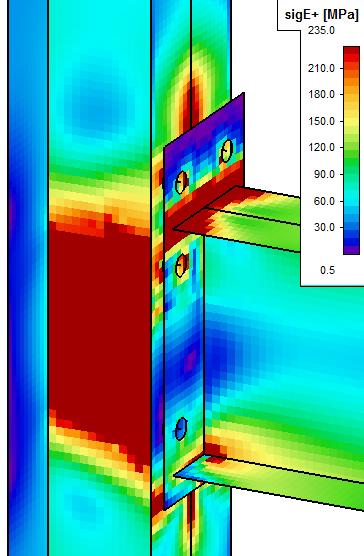
47 Example: Beam_Column_Connection.esa The functionality General Plasticity can also be used to model steel connections using finite elements to perform a plastic stress check. In this example, a bolted column-beam connection is modelled using 2D finite elements in SCIA Engineer. That way the plastic stresses can be calculated by performing a non-linear analysis. Elastic results: Plastic results: 43

48 44

49 Local Non-Linearity The local non linearities can be defined for 1D members, connections between 1D members, 2D members and supports. The following types have been implemented in SCIA Engineer: - Beam local nonlinearity - Beam local nonlinearity including initial Stress - Non-linear member connections - Support nonlinearity - Pressure only elements - 2D Membrane Elements 5.1. Beam Local Nonlinearity also available in the concept edition The options described in this chapter are also possible with a Concept edition. So the Professional edition is not required for this chapter. To input local nonlinearities for 1D members, the functionality Nonlinearity > Beam local nonlinearity must be activated. The non-linearity can then be inputted in the menu through 45

50 The following types are available: - Pressure only - Tension only - Limit force - Gap element All those options are explained with examples in the chapters below Members defined as Pressure only / Tension only Pressure only: the member is only active under pressure (i.e. strut, ) Tension only: the member is only active under tension (i.e. anchor, diagonal, ) When using this type of beam non-linearity, it can happen that numerically a very small pressure/tensile force remains in the member, mostly due to the self-weight. This value will always be negligible compared to the other force components in the member. Example: Tension_Only.esa A 2 nd Order calculation is executed using Newton Raphson, including global imperfections. The diagonals are designated as Tension-only members. The normal forces for a linear analysis show that extreme compression results are obtained in the diagonals. This will inevitably lead to failure due to buckling. 46

51 The normal forces for the non-linear analysis shows that diagonals are now only subjected to tension thus buckling will not occur anymore. Only very small compression forces will appear in the diagonals. Notes: - It is important to keep in mind that Tension only does not change anything for shear forces and moments. The only component which cannot occur is compression, but the member can still be subjected to bending, torsion,... To specify that a member can only be subjected to normal forces, the FEM type of the member can be set to axial force only. 47

52 When using this, the user must be absolutely sure that bending effects cannot occur in reality! -The Calculation protocol for the Nonlinear calculation shows extra information concerning the applied nonlinearities, number of iterations per combination, Example: Mechanism.esa When using Beam Nonlinearities, it is important to make sure that not too many elements are eliminated. A common error is the creation of a mechanism due to the fact too many elements have been designated tension only/pressure only and thus no solution can be found. This principle is illustrated in the following project. A steel frame has been modelled with hinged connections between the elements. The diagonals have been specified as Tension only. 48

53 Due to for example a roof load, both diagonals are subjected to compression. This is not possible for Tension only members so both members are eliminated causing a global instability of the frame Members with Limit Force A member with limit force acts in the structure until a specified limit is reached after which the member will be eliminated from the calculation or yields plastically. The Direction is used to specify in which zone the limit acts: the tension zone or the compression zone. When the limit is reached, it can be specified in the Type field how the member should act. The member can be eliminated from the structure (Buckling) or the member can stay in the structure but with the limit force as maximal axial force (Plastic yielding). The limit itself is defined in the field Marginal Force. A negative value must be specified for a compression limit and a positive value for a tension limit. 49

54 Example: Limit_Force.esa In this project, a frame is modelled in which one diagonal has a compression limit of -30 kn. For the left frame, the type is set to Buckling, for the right frame the type is set to Plastic yielding. A linear analysis shows the following normal forces in the diagonals of both frames: A non-linear analysis, taking into account the limit force gives the following results for the normal forces: In the left frame, the diagonal has buckled so the tensile force in the remaining diagonal is augmented. In the right frame, the diagonal stays in the structure but yields plastically and thus acts at the limit force of -30 kn. The deformed structure for the non-linear analysis shows the following: 50

55 Due to the fact one diagonal has buckled in the left frame, larger horizontal deformations occur Members with gaps There are various connection and support conditions used in a real structure. It may happen that a beam is not attached rigidly to the structure but "starts its action" only after some initial change of its length. The beam thus has to have a certain translation in its local x-direction before it becomes active. This behaviour can be inputted using gap elements. The Type field is used to specify if the member is active only in compression, only in tension or in both directions. The value of the translation can be inputted in the Displacement field. The gap can be defined at the beginning or at the end of the beam using the Position field. Gap members in tension only can for example be used to model a rope: the rope can only work in tension but becomes active only after a certain translation. Gap members in both directions are frequently used in scaffolding structures Beam Local Nonlinearity including Initial Stress To input local nonlinearities for 1D members, including initial Stresses, following functionalities must be activated: - Nonlinearity - Nonlinearity > Beam local nonlinearity - Nonlinearity > 2 nd Order Geometrical nonlinearity 51

56 - Initial Stress and - Cable The non-linearity can then be inputted in the menu through Two extra types are now available: - Members with Initial Stress - Cable Elements 52

57 5.2.1 Members with Initial Stress Tensile forces in elements augment the stiffness of the structure. Compression forces reduce the stiffness. Initial Stress is regarded as follows: - The element in question is taken from the structure. - The initial Stress is put on the element through the defined axial force. - The element is put back into the structure. It is clear that, when the element is inserted into the structure, the initial stress will partly be given to other members thus the inputted force will not stay entirely in the member in question. Notes: - A positive axial force signifies a tensile force; a negative axial force signifies a compression force. - Initial Stress is mostly used in conjunction with a 2 nd Order analysis. To take the inputted Initial Stresses into account for the calculation, the options Initial Stress and Initial Stress as input must be activated through Calculation, Mesh > Solver Setup. Example: Initial_Stress.esa In this project, a simple frame is modelled. The diagonal has a RD30 section and is given an Initial Stress by means of a tensile force of 500 kn. 53

58 In the left frame, the Initial Stress will immediately be distributed to the column. In the right frame, the extra support will prohibit this. A non-linear analysis, taking into account the initial stress gives the following results for the normal forces: As specified, in the left frame, the initial stress is immediately distributed to the rest of the structure so the tensile force of 500 kn is not found entirely in the diagonal. In the right frame, the force cannot be distributed due to the support so the 500 kn stays in the diagonal. This principle is even clearer when looking at the deformed mesh for the non-linear analysis: In theory, when using correctly defined values of the cross-section properties (surface A, moment of inertia I, modulus of Young E), a Beam non-linearity with Initial Stress can also be used to model straight cables with large pre-stress forces. Both Timoshenko and Newton-Raphson methods can be applied in this case. 54

59 In general however, for cables the use of the specific Cable element is advised in conjunction with the Newton-Raphson method Cable Elements Not available in the Professional edition This options needs module esas.12 and this module is included in the expert edition. A Cable element is an element without bending stiffness (Iy and Iz 0). During the solving of the equations this is taken into account so no bending moment will occur in the element. The displacements (in the intermediate nodes) have thus been calculated without bending stiffness. A Cable element allows a precise analysis of cables. For slack cables, SCIA Engineer allows the definition of the initial curved shape of the cable. A cable can be defined in three ways: 1) A Straight cable. 2) A Slack cable with an initial shape caused by the Self-weight. 3) A Slack cable with an initial shape caused by a distributed load Pn. A straight cable is defined by choosing the option Straight at Initial mesh When choosing Calculated for Initial mesh, the cable acts as slack. 55

60 The initial shape will be in equilibrium in relation to the specified load on the cable: either the Selfweight or a distributed load Pn. When activating the option Self weight the specified load will be the self weight of the cable. When choosing for a distributed load Pn, it can be specified that the load is not vertical but is rotated. This can be inputted through the angle Alpha x, the rotation angle around the local x-axis. For a default slack cable this parameter will be zero. When using a calculated initial mesh, the program generates a curves mesh, defining an arc of circle based on the two ends of the member and the sag in the middle of the member. The sag is calculated as follows: = tension in the cable (positive value) = offset of cable at mid-span = span length = line load on the cable (positive = downwards) applied perpendicularly to the axis of the member. can be equal to or or The user can thus define a specific initial shape by specifying the value for the sag f. Using the above formula, this leaves two unknowns: Pn and N. By choosing the value for one, the other is defined and the initial shape is known. 56

61 Note - the distributed load q is always perpendicularly to the member axis. The reason for that is, that only the component of the load that is acting perpendicularly to the beam is affecting the calculation of the sag. However, this implies that the value of sag will be overestimated when the member is not horizontal. Workaround: disable the self weight and input it as instead, with where is the angle between the member axis and the horizontal plane. - There is a limit value for the sag value. The program will not apply a sag value larger then. If the result of the formula above is higher, will be used. - The input of the cable element only defines the initial shape. Afterwards the cable can be loaded by real loads. - The calculations are executed on the deformed shape. This indicates that the eventual deformation of a cable is calculated from the slack shape and not from the initial straight shape. - The deformed mesh can be used to show the true deformation of the cable. - For a precise analysis, the finite element mesh on a cable element needs to be refined. To avoid unnecessary refinements for all members of the structure, the mesh of cable elements can be refined separately through Setup > Mesh > Average size of cables, tendons, elements on subsoil. Example: Cable_Equilibrium.esa In this project, a cable analysis is performed once with a pre-stress force and once without. The cable has following properties: Length of the cable: 20 m Section of the cable: m² E-module of the material: N/m² Loading q on the cable: 1 kn/m Result of SCIA Engineer for initial pre-stress N init =1000 kn w max = 49.8 mm N = kn Check: 57

62 - Moment in the middle of the cable: - Normal force in the cable: For the calculation of the strain, the shape of the displacement is taken as parabolic. This gives the following formula: s b The strain in the cable can then be written as: h N = N init + N d = 1000 kn kn = kn kn Result of SCIA Engineer for initial pre-stress N init = 0 kn Check: w max = mm N = kn - Moment in the middle of the cable: - Normal force in the cable: N = N d = kn The deformation of both cables is shown in the following figure: 58

63 The following results are obtained for the normal forces in the cables: Example: Cable_Polygonal.esa In this benchmark project a polygonal cable is loaded by a Point Load. The value of the Point Load is altered between 3 kn, 5 kn, 10 kn, 15 kn and 20 kn. For each case, the maximal deformation and the normal force are compared with benchmark results from Petersen, ref [9]. The following graphs give an overview of the obtained results out of SCIA Engineer: 59

64 The following table gives an overview of the obtained results in comparison with Peterson: F 3.0 kn 5.0 kn 10.0 kn 15.0 kn 20.0 kn N Petersen [kn] N SCIA Engineer [kn] f Petersen [m] f SCIA Engineer [m] Example: Cable_Distributed.esa In this benchmark project a pre-stressed cable is loaded by a Distributed Load. The value of the distributed load is altered between 1.7 N/m and 6.33 N/m. For both cases, the maximal deformation and the normal force are compared with benchmark results from Petersen, ref [9]. The pre-stress force in the cable is 3,8 kn. The following table gives an overview of the obtained results: q 1.7 N/m 6.33 N/m N Petersen [kn] N SCIA Engineer [kn] f Petersen [m] f SCIA Engineer [m] Example: Cable_InitalShape.esa To illustrate the calculation of the initial shape, a simple cable element is modelled with following properties: Length of the cable: 20 m Section of the cable: m² E-module of the material: 2.1 x N/m² 60

65 The initial shape will be calculated with following properties: Normal force: Distributed load: 200 kn 10 kn/m Afterwards the cable is loaded by a line force of 1kN/m. SCIA Engineer gives the following results for the displacement in the z-direction: Those are the displacements of the distributed load of 1kN/m. This initial shape can also be calculated with following formula: The total deformation in the middle of the cable is than: 61

66 Total deformation = -2500mm mm = mm: Example: Guyed_Mast.esa To illustrate the application of cables, a guyed mast is modelled. The mast is supported by several cables which have a pre-stress force of 5 kn and an initial shape due to the self-weight. The deformed mesh for Non-Linear combination NC9 for example shows the following: 62

67 Detailed calculation information can be found in the Calculation Protocol: 63

68 5.3. Non-Linear Member Connections When inputting hinges on beam elements, it is possible to input a non-linear function for each degree of freedom (ux, uy, uz, fix, fiy, fiz). The function can signify the relation between moment and rotation or force and displacement. When using non-linear functions, it is very important to input a relevant linear stiffness. This value is used during the first iteration of the non-linear calculation (and during a linear calculation). The non-linear functions can be defined through > > 64

69 For member connections, the non-linear functions can be defined for translation or rotation. When defining a function, it is very important to check the signs of the function values. The defining magnitudes for non-linear rotation functions are the internal forces, for non-linear translation functions the displacements. This implies that these functions are inputted in the first and third quadrant. For the end of the function, it is possible to select one of three options: - Free: When the maximal force is reached, it stays at that value and the deformation will rise uncontrolled. - Fixed: When the maximal deformation is reached, it stays at that value and the force component will rise. - Flexible: The relation between force component and deformation is linear. SCIA Engineer also allows creating a new function from the already defined functions to provide an easy input of complex functions. Example: Connection.esa In this example, an industrial hall is calculated using algorithms to calculate the moment-rotation diagram for bolted and welded beam-to-column connections. SCIA Engineer allows the calculation of these diagrams and the automatic application of the diagram as a non-linear spring function for member connections. For the theoretical background, reference is made to the Advanced Training Steel and ref. [14]. The geometry of the structure is shown in the following figure: The structure is calculated in 2 nd Order using Timoshenko s Method. The diagonals have been set as Tension-only. In node N2 a bolted beam-to-column connection is modelled: 65

70 The Moment-Rotation diagram is calculated by SCIA Engineer using the algorithm of the EN Together with the calculated diagram, automatically a non-linear function is created: 66

71 The function characterizes both tension-on-top and tension-at-bottom. This function can then be assigned to the hinge defined in node N2: 5.4. Support Nonlinearity SCIA Engineer allows the following types of non-linear supports: - Tension only / Pressure only supports - Nonlinear springs for supports - Friction supports 67

72 Tension only / Pressure only Supports To input nonlinearities for supports, the functionality Nonlinearity > Support nonlinearity must be activated. Supports with tension can be automatically eliminated. This is mostly used for slabs on subsoil, column bases of for example scaffoldings, struts, The following types of supports can be eliminated if tension occurs: - Nodal Support - Line Support - Subsoil For Nodal Supports or Line Supports it is possible to specify a translation degree of freedom as Rigid pressure only or Flexible Pressure only. Subsoils are always regarded as Pressure-only for a non-linear calculation. No specific input has to be made. 68

73 Example: Subsoil.esa In this example, a slab on subsoil is calculated. The slab is loaded by a Point Force in the middle. The deformed mesh for the linear analysis shows the following: Especially in the corners, tensile contact stresses are expected: A non-linear analysis, taking into account the pressure-only characteristic of the subsoil shows the following deformation: 69

74 As can be seen, the slab will rise at the corners so no more tensile contact stresses are obtained: The pressure stresses in the middle have increased which is expected when the slab can rise at the corners. Note: - When using subsoil, it is important to adequately refine the mesh in order to produce precise results. - When calculating following the Winkler theory, the Pasternak values (C2) must be set to zero Nonlinear Springs for Supports As seen for nonlinear member connections, it is also possible to use non-linear functions for supports. For each degree of freedom (X, Y, Z, Rx, Ry, Rz) a nonlinear function can be inputted. The function can signify the relation between moment and rotation or force and displacement. 70

75 When using non-linear functions, it is very important to input a relevant linear stiffness. This value is used during the first iteration of the non-linear calculation (and during a linear calculation). The definition of the nonlinear functions is exactly the same as seen with nonlinear member connections. In addition to nodal supports, a non-linear function can also be used for a subsoil under a plate. Example: Support_Function.esa In this example, the use of a non-linear function for a support is illustrated. A simple beam on two supports is modelled. The translation Z of both supports has been defined as a non-linear function: 71

76 The beam is loaded by a point force at one end. The value of the point force is taken as 1kN and 1.4kN. A non-linear analysis shows the following deformation for the load of 1kN: This value can manually be approximated as follows: 100mm U z ( 1000N 628N) 53, 14mm 1328N 628N For the load of 1.4 kn, the fixed end of the function is reached thus the maximal deformation of 100mm is obtained: 72

77 Example: Pallet_Racking.esa In this example, the calculation of a pallet racking system is shown according to ref. [10] Eurocode ENV and ref. [11] FEM This last reference gives field test methods which allow the definition of moment-rotation diagrams for beam-to-column connections and column supports. The beam-to-column connections and column supports can be defined by means of non-linear functions. The following non-linear spring is defined for the column supports: The beam-to-column connections are defined by the following non-linear characteristic: 73

78 Example: Culvert.esa This project illustrates the use of non-linear functions to model for example the soil under a culvert. The culvert has the following shape: Non-linear supports have been defined with appropriate functions to model the behaviour of the soil: 74

79 A non-linear analysis gives the following deformation pattern for combination NC2: Friction Supports Friction supports can be used to model the fact that a reaction component is dependent on another component. The horizontal component is for example dependent on the vertical component. When the friction force is surpassed, the support slips through resulting in large deformations. To input friction supports, both the functionalities Nonlinearity > Support nonlinearity/soil spring and Friction Support/Soil spring must be activated. 75

80 When entering a nodal support, the option Friction can be chosen for the translational degrees of freedom (X, Y, Z). The option From Reaction is used to specify which force component causes the friction force. X, Y, Z: The final limit force can be calculated from the reaction in a specified direction. If a support in the X-direction is being defined, it can be said that the friction force should be determined from the reaction calculated in either the Y or Z direction. The friction force is calculated from the following formula: mju x R z XY, XZ, YZ: The final limit force can be calculated as a compound friction. Only one of the stated options is offered for each direction. E.g. if a support in the X-direction is being defined, it can be said that the friction force should be determined from the reactions calculated in the Y and Z direction. The friction force is calculated from the following formula: 76

81 mju x R 2 y R 2 z X+Y, X+Z, Y+Z: The same as above applies here. A different procedure is however used to calculate the limit force. E.g. for a friction support in the X-direction the following formula is employed: mju x R y mju x R In these formulas, mju specifies the coefficient of friction. In the field C flex, the stiffness of the support can be inputted. z Note: - Friction can be inputted in one or two directions. It is not possible to define friction in all three directions since otherwise the "thrust" cannot be determined. - When simple friction (X, Y, Z) is defined in two directions, the option Independent is available. This specifies that the friction in one direction is independent on the friction in the other direction. - Composed friction (e.g. YZ or Y+Z) can be specified only in one direction. Friction supports can be used for several types of structures. Nearly every support which isn t rigidly connected to the surface on which it stands is subjected to friction. Examples include base jacks of scaffolding structures, supports on an inclined surface, pipes in boreholes, Example: Scaffolding.esa This project illustrates the use of friction supports for a scaffolding structure. The scaffold has the following geometry: The base jacks are inputted as friction supports. Since a base jack, by default, is not connected to the surface, the Z-direction is defined as rigid Pressure-only. Both horizontal degrees of freedom X and Y are defined as Friction, dependent on the reaction Z. 77

82 When large wind loads are taken into account, for example due to netting, large horizontal reaction forces are expected in the base jacks. When these reactions surpass the friction force, the support slips through. After a non-linear analysis of the scaffold, the deformed mesh for combination NC5 shows the following: In the middle base jacks, the friction force is clearly surpassed and thus the supports slip through. To avoid this, the reaction in Z-direction must be augmented thus extra dead weight like ballast will be required or the base jacks must be fixed to avoid slipping. Note: The functionality Nonlinear Line Support defines a specific type of soil spring developed for the Pipfas project (Buried Pipe Design). 78

83 5.5 2D Elements D Membrane Elements Not in Professional Edition This option is implemented in module esas.37 and included in the Expert edition. So with the Professional edition the option of Membrane elements as described in this chapter, will not be possible. Membrane elements are defined as shell elements which have no flexural stiffness and no axial compression stiffness. Membrane elements can thus be used to model canvas, nets, etc. that are subjected to axial tension. To obtain realistic results, a 2 nd Order calculation needs to be executed using the Newton-Raphson method. To input 2D membrane elements, the functionalities Nonlinearity > 2 nd Order Geometrical nonlinearity and Membrane Elements must be activated. When defining the 2D element, the option Membrane must be chosen as FEM nonlinear model. 79

84 Note: - Membrane elements can only be modelled in a General XYZ environment. - Due to the fact the flexural rigidity is zero, no ribs, orthotropic parameters or physical non-linear data can be inputted on a membrane element. - Since a membrane element has no axial compression stiffness, no concrete calculation can be performed on this type of element. Example: Membrane.esa In this project, a textile canvas is modelled. At the four corners of the canvas, steel cables are attached. Two cables are subjected to a tensile force of 50kN in horizontal direction. Since the canvas has an initial position 0,5m lower than the endpoint of the cables, the canvas will first be pulled straight. Since both cable and membrane elements are used, a 2 nd Order non-linear analysis is executed using the Newton-Raphson method. The deformed mesh for the non-linear analysis shows that the canvas has been pulled straight: 80

85 When the scale of the results is augmented, the typical deformation of the membrane element can clearly be seen: The tensile forces for the cable elements are shown on the following figure: 81

86 The principal membrane force n1 shows the tensile forces in the canvas: In the same way, n2 can be shown: The results show the 2 nd Order effect: due to the tensile forces in one direction, the canvas obtains a stiffness which results in compression membrane forces. 82

87 Pressure only To input pressure only for 2D elements, the functionality Nonlinearity and Press only 2D members must be activated. With this option, tension in 2D elements can be automatically eliminated. This is mostly used for masonry elements. In below some examples are shown to clarify this option. Example: PressureOnly1.esa This project illustrates the use of pressure only elements. In this project two 2D-elements are modelled. The first one is modelled as an isotropic element with no nonlinearity, the second one is a pressure only element: 83

88 When calculating those elements, for every mesh element a certain orthotropy will be inserted. At the first iteration step all the pressure only elements, will be calculated as an isotropic element. After the first calculation, SCIA Engineer will input another stiffness on all elements in tension. So a certain orthotropy will be created. With this stiffness the tension capacity of this element will decrease. After adapting the orthotropic parameters a new calculation will be performed. After this second iteration step again the elements in tension will get another stiffness. This process will be repeated until equilibrium is reached. The difference between the isotropic and orthotropic elements can be clearly view looking at the normal force ny for these members: In these results the real pressure of this element is visible for the right element. Looking at the trajectories of this normal force, the trajectory of the pressure force will be even more visible: 84

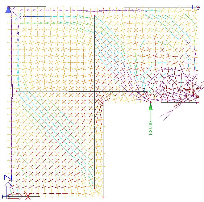
89 Example: PressureOnly2.esa When looking at the pressure diagonals in a reinforced 2D concrete element, ribs can be imported as reinforcement. In this example a plate with a bearing support is inserted with two ribs acting as the reinforcement of the plate: Looking at the results of this 2D element, the pressure diagonals inside this element are clearly visible: 85

90 86

91 Stability Calculations A stability calculation calculates the global buckling mode (eigenmode) of a structure under the given loading. In addition, the ratio between the buckling load and the applied load is given. Stability calculations are used to obtain an insight into the buckling mechanisms of a structure, to calculate the buckling length of a member for use in the Steel Code Check, to verify if 2 nd Order calculations are required, 6.1 Stability Combinations As seen for a non-linear analysis, the principle of superposition is also not valid for a Stability calculation. The combinations have to be assembled before starting the calculation. In SCIA.Engineer, this is done by defining Stability Combinations. A stability combination is defined as a list of load cases where each load case has a specified coefficient. As specified for the non-linear combinations, it is possible to import the linear combinations as stability combinations. 6.2 Linear Stability During a linear stability calculation, the following assumptions are used: - Physical Linearity. - The elements are taken as ideally straight and have no imperfections. - The loads are guided to the mesh nodes, it is thus mandatory to refine the finite element mesh in order to obtain precise results. - The loading is static. - The critical load coefficient is, per mode, the same for the entire structure. - Between the mesh nodes, the axial forces and moments are taken as constant. The equilibrium equation can be written as follows: 87

92 The symbol u depicts the displacements and F is the force matrix. As specified in the theory of the Timoshenko method, the stiffness K is divided in the elastic stiffness K E and the geometrical stiffness K G. The geometrical stiffness reflects the effect of axial forces in beams and slabs. The basic assumption is that the elements of the matrix K G are linear functions of the axial forces in the members. This means that the matrix K G corresponding to a th multiple of axial forces in the structure is the th multiple of the original matrix K G. The aim of the buckling calculation is to find such a multiple for which the structure loses stability. Such a state happens when the following equation has a non-zero solution: In other words, such a value for should be found for which the determinant of the total stiffness matrix is equal to zero: Similar to the natural vibration analysis, the subspace iteration method is used to solve this eigenmode problem. As for a dynamic analysis, the result is a series of critical load coefficients with corresponding eigenmodes. To perform a Stability calculation, the functionality Stability must be activated. In the results menu, the values can be found under the caption The number of critical coefficients to be calculated per stability combination can be specified under Setup > Solver. Note: 88

93 - The first eigenmode is usually the most important and corresponds to the lowest critical load coefficient. A possible collapse of the structure usually happens for this first mode. - The structure becomes unstable for the chosen combination when the loading reaches a value equal to the current loading multiplied with the critical load factor. - A critical load factor smaller than 1 signifies that the structure is unstable for the given loading. - Since the calculation searches for eigen values which are close to zero, the calculated values can be both positive or negative. A negative critical load factor signifies a tensile load. The loading must thus be inversed for buckling to occur (which can for example be the case with wind loads). - The eigenmodes (buckling shapes) are dimensionless. Only the relative values of the deformations are of importance, the absolute values have no meaning. - For shell elements the axial force is not considered in one direction only. The shell element can be in compression in one direction and simultaneously in tension in the perpendicular direction. Consequently, the element tends to buckle in one direction but is being stiffened in the other direction. This is the reason for significant post-critical bearing capacity of such structures. - It is important to keep in mind that a Stability Calculation only examines the theoretical buckling behaviour of the structure. It is thus still required to perform a Steel Code Check to take into account Lateral Torsional Buckling, Section Checks, Combined Axial Force and Bending, Example: Buckling_Frame.esa A stability analysis is performed on a steel frame. The first three buckling modes are calculated and the buckling loads are compared to the analytical results from ref.[26] to obtain a benchmark for the stability calculation of SCIA Engineer. To obtain precise results, the number of 1D elements is refined through Setup > Mesh. 89

94 Under Setup > Solver the Number of critical values can be specified. In addition, the Shear Force deformation is neglected to have a good comparison with the analytical results. After executing a Stability calculation, the following critical load coefficients are obtained: The corresponding buckling modes can be shown under Displacement of nodes by viewing the Deformed mesh for the Stability Combination. 90

95 Buckling mode 1 Critical load factor = 2,21 Buckling mode 2 Critical load factor = 2,89 Buckling mode 3 Critical load factor = 3,53 The loading F on each column is 100 kn so the critical buckling load N cr can be calculated as: This gives the following results which can be compared to the analytical calculation: N cr for SCIA Engineer Ref.[26] Buckling Mode kn kn Buckling Mode kn kn Buckling Mode kn kn 91

96 Example: Buckling_Arch.esa When calculating for example an arched steel bridge, one of the required parameters for a Steel Code Check is the buckling length of the arch. Using a stability calculation, the buckling factor of any member can be obtained. As an example, a steel parabolic arch is modelled with two fixed end points. The arch has a horizontal length of 10m, height 2m and is loaded by a vertical line load of 30 kn/m. The Shear Force deformation is neglected to have a good comparison with analytical results. Using an Average Mesh size for curved elements of 0,1m, a Stability Calculation yields a critical load factor of 0,46. The first buckling mode has the following shape: 92

97 This result can be checked using an analytical formula from Ref.[28]. The critical lineload for a fixedfixed arch with height 20% of the support distance is given as: With: E = Modulus of Young = N/mm² I = Moment of inertia = ,67 mm 4 L = Distance between supports = mm P cr = 14,448 kn/m The loading P on the structure was 30 kn/m so the critical load coefficient can be calculated as: This result corresponds to the result of SCIA Engineer. Using the critical load coefficient, the buckling load of the arch can be calculated. The minimal normal force N under the given loading is 195,82 kn. The minimal is used since this will give a conservative result for the buckling length. The buckling load N cr can then be calculated as: Applying Euler s formula, the buckling factor k can be calculated: In which s specifies the arch length of 10,982m 93

98 The parameters can now be inputted: This buckling factor can now be inputted in the buckling data of the arch so it can be used for a Steel Code Check. This example illustrates the use of a stability calculation for a simple arch. The same procedure can now be applied to more complex structures like arched bridges, truss beams, concrete buildings, Example: Buckling_Arch_FEM.esa To illustrate the use of stability in finite element calculations, the arched bridge of the previous example is modelled as a shell element. Using an Average Mesh size of 2D element of 0,1m, a Stability Calculation yields the following critical load factor: The corresponding buckling mode can be shown by viewing the Deformed Mesh under 2D Members > Deformations of Nodes 94

99 The result corresponds to the analytical solution shown in the previous example. Example: Buckling_Arbitrary_Profile.esa In this example, the buckling load for a composed column is calculated. The column has a variable section consisting of two different cross-sections. The critical buckling load is compared with the analytical result from Ref.[6]. The loading is taken as 1 kn so the critical load coefficient equals the critical buckling load. To obtain a correct comparison with the analytical calculation, the shear force deformation is neglected: 95

100 The formula for the buckling load of a member with arbitrary cross-section is given in Ref.[6], pp.114 by formula (2-48): With m a parameter depending on the length of the different sections and the ratio I 1 /I 2. This parameter is specified in table 2-10 of Ref.[6]. I mm 4 I mm 4 a 4 m l a/l 0.4 I 1 /I m m 4.22 P cr 3713 kn A Stability Calculation gives the following result: This result corresponds to the analytical solution. The corresponding buckling mode has the following shape: 96

101 Note: The buckling shapes can be animated through View > New Animation Window Example: Stability_EC3.esa As seen during the 2 nd Order calculations, according to EC3 Ref.[27], a 1 st Order analysis may be used for a structure, if the increase of the relevant internal forces or moments or any other change of structural behaviour caused by deformations can be neglected. This condition may be assumed to be fulfilled, if the following criterion is satisfied: Fcr cr 10 for elastic analysis. F Ed With: α cr The factor by which the design loading has to be increased to cause elastic instability in a global mode. F Ed The design loading on the structure. F cr The elastic critical buckling load for global instability, based on initial elastic stiffnesses The factor α cr thus corresponds to the critical load coefficient calculated through a Stability calculation. The frame was regarded in a previous example and had the following geometry: A Stability Calculation gives the following critical load coefficients for the design loading: 97

102 The lowest positive factor of 13,17 has the following buckling shape: Since this lowest factor is higher than 10, this implies that a 1 st Order calculation may be executed; the structure is thus not sensitive for 2 nd Order effects. Example: Stability_Imperfection.esa In Chapter 6, the use of the buckling shape as imperfection according to EC3 was discussed. In this example, the procedure is illustrated for a column. The column has a cross-section of type IPE 300, is fabricated from S235 and has the following relevant properties: E = N/mm² f y = 235 N/mm² M1 = 1.00 L = 5000 mm A = 5380 mm² I y = mm 4 W pl,y = mm 3 98

103 Calculation of the buckling shape First a Stability calculation is done using a load of 1kN. This way, the elastic critical buckling load N cr is obtained. In order to obtain precise results, the Number of 1D elements is set to 10. In addition, the Shear Force Deformation is neglected so the result can be checked by a manual calculation. The stability calculation gives the following result: This can be verified with Euler s formula using the member length as the buckling length: The following picture shows the mesh nodes of the column and the corresponding buckling shape: Using for example an Excel worksheet, the buckling shape can be approximated by a 4 th grade polynomial. 99

104 A polynomial has the advantage that the second derivative can easily be calculated. Calculation of e 0 (Class 2) 0,21 for buckling curve a These intermediate results can be verified through SCIA Engineer when performing a Steel Code Check on the column: 100

105 Or with : The required parameters have now been calculated so in the final step the amplitude of the imperfection can be determined. Calculation of init The mid section of the column is decisive x = 2500 mm cr at mid section = 1000 = 5,659 mm This value can now be inputted as amplitude of the buckling shape for imperfection. To illustrate this, the column is loaded by a compression load equal to its buckling resistance. However, due to the imperfection, an additional moment will occur which will influence the section check. The buckling resistance can be calculated as follows: 101

106 A non-linear combination is created in which the buckling shape as imperfection is specified. Using this combination, a non-linear 2 nd Order calculation is executed using Timoshenko s method. The additional moment can be easily calculated as follows: When performing a Steel Code Check on the column for the non-linear combination, this can be verified. The critical check is performed at 2,5m and has the following effects: The additional moment thus corresponds to the moment calculated by SCIA Engineer. As seen in the diagram, Path 3 is followed: the buckling shape serves as a unique global and local imperfection. This implies that only a section check and Lateral Torsional Buckling need to be checked. Since LTB is negligible with this small bending moment, only a section check is required. This example has illustrated the use of a buckling shape as imperfection. Depending on the geometry of the structure, this imperfection can have a large influence on the results due to the additional moments which occur. When using this method, it is very important to double check all applied steps: small changes to the loading or geometry require a re-calculation of the buckling shape and amplitude before a non-linear analysis may be carried out. As a final note: the buckling shape only gives information about a specific zone of the structure. The imperfection is applied at that zone and results/checks are only significant for that zone. Other combinations of loads will lead to another buckling shape thus to each load combination a specific buckling shape must be assigned and a steel code check should only be used on those members on 102

107 which the imperfection applies. Since the applied buckling shape corresponds to a global mode, failure of these members will lead to a collapse of the structure. 6.3 Non-Linear Stability As specified in the assumptions of the previous paragraph: a Stability calculation is by default a linear process. Non linearities like friction supports, pressure only supports are not taken into account. Specifically for this purpose, SCIA Engineer provides the use of a Non-Linear Stability Calculation. This type of calculation has the following additions to the Linear Stability calculation: - Local Non-Linearities are taken into account - 2 nd Order effects are taken into account using the Modified Newton-Raphson algorithm. Modified Newton-Raphson follows the same principles as the default method but will automatically refine the number of increments when a critical point is reached and will only update its stiffness matrix every N iterations. This method can therefore give precise results for post-critical states. SCIA Engineer will perform a 2 nd Order calculation taking into account Local Non-Linearities. After this calculation, the resulting deformed structure is used for a Stability calculation. As a result, the Critical Load Factor of the structure is obtained for the structure including Non-Linearities. To activate the Non-Linear Stability calculation, the functionalities Stability and Nonlinearity > 2 nd Order Geometrical nonlinearity must be activated. In addition, Support and/or Beam local nonlinearities can also be activated. The choice of the 2 nd Order Theory, the amount of increments and the maximal amount of iterations can be specified through Calculation, Mesh > Solver Setup. 103

108 Since the non-linear stability calculation automatically implies the Modified Newton-Raphson method for the solver, this method cannot be chosen here. The reason why this field is available is to perform a normal 2 nd Order Calculation using Modified Newton-Raphson instead of a Stability Calculation. Since the Modified Newton-Raphson method also applies the loading using increments, it is important to set a right amount of increments. This implies that it is advised to choose the Newton-Raphson method so the user has access to the number of increments. Example: Stability_Falsework.esa In this example, a Stability analysis is carried out on a large falsework structure measuring 15m x 15m x 12m. All diagonals of the structure have been given a gap of 1mm. 104

109 The structure is loaded by its self-weight, formwork and concrete for a total loading of +/ tonnes. First a Linear Stability calculation is carried out to evaluate the critical load factor. The number of 1D elements is set to 5 to obtain good results without severely augmenting the calculation time. The following result is obtained: The critical load factor is smaller then 10 which indicates that the structure is susceptible to 2 nd Order effects. Therefore a 2 nd Order calculation is carried out using Newton-Raphson. The number of increments is set to 5 and the maximal number of iterations is set to 50. The 2 nd Order calculation leads to the following message: 105

110 This implies that the 2 nd Order calculation does not converge to a result but leads to instability. The question now rises as to what causes this instability. This is the point where the Non-Linear Stability calculation comes in. During the Linear Stability Calculation, the Gap elements on the diagonals of the structure were not taken into account. A Non- Linear Stability calculation takes into account both 2 nd Order effects and the Gap elements. The Non-Linear Stability Calculation gives the following result: This result gives a very important conclusion: the structure including all Gap elements is not capable of supporting the loading. Only 40% of the loading can be supported before instability occurs. This is the reason why the 2 nd Order calculation does not pass. 106

111 When Local Non-Linearities are used, it is mandatory to execute a Non-Linear Stability calculation to draw correct conclusions concerning the global buckling of the structure. 107

112 7. Troubleshooting In this final Chapter, some common failure messages are given which can occur during a non-linear analysis. 7.1 Singularity Singularity problems occur frequently during a non-linear calculation. Messages of the following type are generated by SCIA Engineer: The singularity can be checked by running the check of singularities: 108

113 The cause of these messages can be the following: - The structure is a mechanism: check supports, hinges, unconnected members, - The structure becomes a mechanism by eliminating elements (members, supports, ) Examples include tension only diagonals which are all eliminated, a subsoil (only compression) which comes entirely under tension, - The structure becomes unstable due to the creation of plastic hinges. - The entire structure or part of it buckles. In the stiffness matrix this implies that K G > K E - The instability is caused due to small section properties of manually inputted cross-sections. In many cases, the torsional resistance I t is too small. - As explained in the theory, the Timoshenko method is not suitable when the normal force in a member is larger than its critical buckling load. In this case, Newton-Raphson should be applied. To find out which cross-section causes this problem, the sections can be modified alternately until the 2 nd Order calculation passes. 7.2 Convergence If, during a non-linear analysis the criterion of convergence is not met, messages of the following type are generated by SCIA Engineer: The cause of these messages can be the following: - Too few iterations have been specified in the Solver Setup. - The structure is close to instability. - Cyclic elimination of members or supports: the elements are eliminated during an iteration and are re-instated during the following iteration. - To examine this in detail, the calculation can be executed for for example three iterations: take iteration i-1, i and i+1 and compare the results. In these results, there will be a difference in one member (for example in one iteration the member is in tension, in the following iteration it is in compression). - If the non-linear stability calculation does not converge, make sure 2 nd Order is activated as functionality. 109