Tutorial 6. Pumping Well and River

Transcription

1 Tutorial 6 Pumping Well and River Table of Contents Objective. 1 Step-by-Step Procedure... 2 Section 1 Data Input. 2 Step 1: Open Adaptive Groundwater Input (.agw) File. 2 Step 2: Pumping Well Design Database 3 Step 3: Assign Pumping Well to Model. 4 Step 4: Assign Pumping Well to Model (cont.). 6 Step 5: Save Pumping Well Data.. 6 Step 6: Assign Groundwater Recharge.. 7 Step 7: River Boundary Condition. 8 Step 8: Add Groundwater Pathline 9 Step 9: Assign Hydraulic Head and Solute Concentration Monitoring Points.. 11 Step 10: Review Model Input Data and Boundary Conditions 13 Section 2 Simulation Results Visualization.. 15 Step 1: View 2D Plan View Hydraulic Head Contour (Line) Map Step 2: Contour Options. 16 Step 3: View Zoom and Translate.. 18 Step 4: Contour Map Overlays and Pore Velocity Vectors 18 Step 5: Cross-Section (x-z) View of Hydraulic Head Distribution 19 Step 6: View Solute Concentration Output and Monitoring Point Data 20 Step 7: Solute Concentration Cross-Section (x-z) View with Pathline.. 22 Step 8: 3D Plume Volume Plot with Blanking Objective Illustrate the incorporation of a pumping well in combination with a river boundary condition. The completed Adaptive Groundwater input files for this tutorial are included in the Tutorial_6 subdirectory of the tutorials directory under the Adaptive_Groundwater program folder: C:\Adaptive_Groundwater\Tutorials\Tutorial_6\Tutorial_6_Completed.agw 1

2 Because Tutorial 6 builds upon the input data and boundary conditions for Tutorial 1, you can refer to this first tutorial for illustrations of basic input data preparation (e.g., grid design, basic boundary condition specification, time step control, etc.). The completed Tutorial 6 project files are provided to you as a reference (you can check the completed input data if you have questions while working through the tutorial). Many output times are also provided so that you can view the variations of hydraulic heads and solute concentrations over a long time period. As discussed below, you will work with a separate set of project files. This tutorial is divided into two sections. The first part covers these data input options: pumping wells, monitoring points, and groundwater pathlines. Section 2 illustrates the generation of various two- and three-dimensional visualizations of the simulation results for this tutorial. Step-by-Step Procedure Section 1 Data Input Step 1 - Open Adaptive Groundwater Input (.agw) File Go to File > Open in the main menu to open the file Tutorial_6_Start.agw that is stored in the following subdirectory: C:\Adaptive_Groundwater\Tutorials\Tutorial_6 The Base Grid is initially displayed on the screen (Figure 1). 2

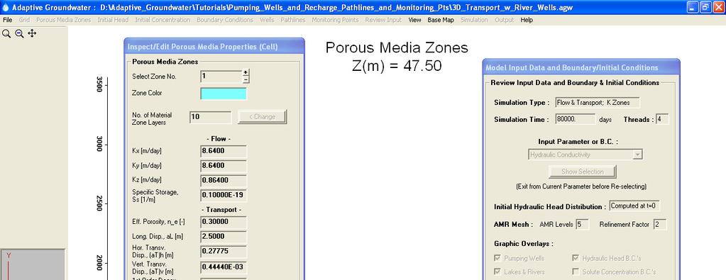
3 Figure 1 Step 2 Pumping Well Design Database We start by reviewing the pumping well design database. In the main menu select Wells > Edit/View Well Database to pop up the well design dialog shown in Figure 2. The database contains one well design (no. 2): a vertical, partially-penetrating extraction well with a fivemeter well screen located at the top of the aquifer. The groundwater extraction rate increases from an initial value of m 3 /day to 545 m 3 /day at t = 2 years and thereafter. Since this is an extraction well, the Injection Concentration is not used in the simulation and is set to an arbitrary negative value of -1. Note: well design number one is intentionally left blank to represent no well. If you want to review a full discussion of the parameter values for this dialog select the Help button. 3

4 Figure 2 Step 3 Assign Pumping Well to Model Close the well database dialog and on the main menu select Wells > Assign Pumping Wells to display the Assign Wells dialog (Figure 3). Use the Select Layer No. options ( +/- buttons or Go To button) to change the displayed layer to 10. 4

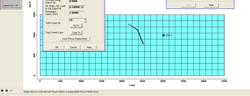
5 Note: When viewing the grid in plan-view (x-y) mode, any Base Grid layer may be displayed when assigning pumping wells ( Select Layer No. in Figure 3). However, in cases such as this one where the partially-penetrating well screen is vertically-oriented and lies only within a single layer (e.g., Layer 10) the well location symbol is plotted only when the pumping layer is displayed. The Review Input option (main menu) does show all well symbols regardless of the displayed layer (see example below). Alternatively, you can assign pumping wells while in cross-section view mode (i.e., x-z or y-z slices) so that, for example, vertical well screens would be displayed over their entire length. Figure 3 5

6 Step 4 Assign Pumping Well to Model (cont.) Using the left mouse button assign an extraction well to the approximate location shown in Figure 4 (x = m, y = m). As this figure illustrates, when you left-click on the desired well location a second dialog pops up where, if you want to, you can directly enter (or fine tune ) the final well coordinates and change the well name. The allowable well coordinate adjustment ranges (X min /X max and Y min /Y max ) are defined as the boundaries of the Base Grid cell that contains the well. As discussed in the help documentation, well-screen fluxes are assigned to the finest cells (i.e., the highest level of AMR refinement) that are intersected by the well screen. Therefore, the well location and screen length should be carefully selected. Click OK to complete the well assignment or Cancel to abort the well placement. Step 5 Save Pumping Well Data Make to sure to Save your well assignment before exiting this option. Click Cancel in the Assign Wells dialog to return to the main menu without saving your pumping-well input. Figure 4 6

7 Step 6 Assign Groundwater Recharge On the main menu select Boundary Conditions > Recharge Rate and Concentration > Assign > Polygon to load the Assign Uniform Recharge zones dialog (Figure 5a). Change the zone number to 2 (recharge rate = 0.06 m/yr; recharge concentration = 0 mg/l) and assign Zone 2 to the entire model domain by left clicking a polygon that surrounds the entire grid. Push the right mouse button to complete the polygon ( Esc key to abort). Select the Save Recharge Zones button to save these values. Figure 5a 7

8 Step 7 River Boundary Condition Specification of the river boundary condition used in this tutorial was illustrated in Tutorial 5. To view this river B.C., select Boundary Conditions > River or Lake > River > Inspect in the main menu (Figure 5b). This displays the Inspect/Edit River Boundary Conditions dialog box (Figure 6). Figure 5b 8

9 Figure 6 Step 8 Add Groundwater Pathline Close the river inspection dialog and begin the specification of a groundwater pathline starting point by selecting Pathlines > Assign in the main menu (Figure 7). The Assign Pathline Starting Coordinates dialog appears (Figure 8). Change the current layer to 6. Leave the default pathline direction as forward (i.e., track downgradient in the direction of flow) and keep the very large pathline stop time (i.e., track throughout the simulation). With these pathline parameters, place a pathline starting point (left click) in the approximate location shown in Figure 7 (center of the Gaussian starting plume). After clicking on the starting point, the Finalize Pathline Starting Coordinates pops up; enter the final coordinates shown in Figure 9. 9

10 Make to sure to save your selections ( Save Pathlines ) before exiting this option. You can Cancel to abort the pathline definition without saving your input. Figure 7 10

11 Figure 8 Figure 9 Step 9 Assign Hydraulic Head and Solute Concentration Monitoring Points Four monitoring points have been assigned (Monitoring Points > Assign; Figure 10) at different depths in the aquifer along the three-dimensional plume trajectory [Figure 10 (plan view) and Figure 11 (x-z slice)]. Similar to pumping well and pathline assignments, the monitoring point coordinates can be fine-tuned using the Finalize Monitoring Point Information dialog (Figure 11). 11

12 To inspect these monitoring points, select Monitoring Points > Inspect in the main menu (Figure 10). Figure 10 12

13 Figure 11 Step 10 Review Model Input Data and Boundary Conditions You can review the model input data and boundary conditions at any time by selecting Review Input on the main menu, which pops up the dialog box in Figure 12. Push Show Selection to inspect an input data type or boundary condition from the drop-down menu (left click on a B.C. or material zone to view the input values). Use the checkboxes to add desired B.C. overlays to each plot. In this example, we show Hydraulic Conductivity (one uniform K zone) with overlays of the hydraulic head (linear head B.C. s at the left- and right-hand side aquifer boundaries), the river, and the extraction well for this tutorial (plan view of top layer: Figure 13; x-z cross-section at y = 975 m with 10x vertical exaggeration: Figure 14). The solute concentration B.C. s checkbox is not activated in Figure 12 because inflow concentrations at aquifer boundaries are set to the default value of 0.0 (Boundary Conditions > Default Inflow Concentrations). 13

14 Figure 12 Figure 13 14

15 Figure 14 Section 2 Simulation Results Visualization In this section we show how to create various two- and three-dimensional plots of the simulation results for Tutorial 6. You can use either the supplied Tutorial_6_Completed project files or your working copy of the Adaptive Groundwater files for this tutorial: Tutorial_6_Start.agw. It does not matter if you have made new runs with shorter simulation times than those shown here; select whatever output time that you want. Step 1 View 2D Plan View Hydraulic Head Contour (Line) Map In the main menu select Output > Hydraulic Head and the View Simulation Results dialog appears (Figure 15). A plan-view flood map through the middle of the aquifer is automatically generated. Click the Go To button at the top of the dialog to pop up a child dialog with 15

16 available output times; click on any output time you want and select OK in the Go to Output Time dialog. You may also use the + / - buttons to toggle through the output times. Under Plot and Contour Types you see that 2D (i.e., two-dimensional) plots are the default. Change the Contour Type to lines. Figure 15 Step 2 Contour Options Use the slice plane Go To button (Figure 15) to change the view-plane elevation to m and the plot in Figure 16 is generated. You can also click the Layer no. +/- buttons (Figure 15). Further, you can view an animation of the different plan-view slices by changing the Animation Type to Layer (K-plane) and clicking the Start Animation button. A total of 40 head contour intervals are used in the range 45.0 to 54.5 m. To change the contour intervals select Contour Options in the View Simulation Results dialog and click the Contouring Options tab in the Contour Parameters and Overlays child dialog (Figure 17). 16

17 Note: the layer number refers to the Adaptive Mesh Refinement (AMR) mesh associated with the multi-level AMR grid created during the simulation. In highly-refined mesh areas the vertical discretization is equal to the grid spacing in the highest-level subgrid (e.g, Level 5 in this example which utilizes five AMR levels). In less-refined areas the grid layer thickness for the output is equal to the grid spacing in the most-refined subgrid (e.g., Level 1, 2, 3, or 4). Figure 16 17

18 Figure 17 Step 3 View Zoom and Translate Figure 18 is a close-up plan-view plot of the hydraulic head contours and pore velocity vectors (activate under the Vectors tab in the Contour Options dialog) in the vicinity of the river and extraction well. You can vary the vector length [V Length (%)] and reduce the number of plotted vectors by changing the Vector Indices Skip parameters to values greater than one (Figure 18). In all plots you can Zoom In, Zoom Last, or Translate the view by clicking one of the icons in the upper-left corner of the display (Figure 16) or by making the appropriate selection under View in the main menu. If you wish to use any of these display options later, click on the Save Plot Format button at the bottom of the View Simulation Results dialog (Figure 15). Step 4 Contour Map Overlays and Pore Velocity Vectors Figures 16 and 18 also consist of these overlays: the AMR mesh, the groundwater pathline, the river, and the extraction well. The mesh overlay can be turned off by un-checking the Mesh box in the Contour Options dialog (under the Overlays tab; Figure 17). If groundwater pathline starting locations are defined (as in this case) their computed trajectories can be shown in the output by checking the Show Pathlines box in the Contour Options dialog 18

19 (under the Pathlines tab; Figure 17). Display overlays of pumping wells and rivers by checking Wells and River & Lake B.C. s, respectively, under the Overlays tab. Figure 18 Step 5 Cross-Section (x-z) View of Hydraulic Head Distribution To display the cross-sectional view in Figure 19, click on the X-Z Slice (Row) button in the lower left hand corner (red circle in Figure 16), and then select the row of cells (i.e., x-z slice) that cuts through the extraction well (or select View > Change View Plane in the main menu). When you first switch to the cross-section view, you will want to add vertical exaggeration (e.g., VE = 10-20) by going to View > Vertical Exaggeration in the main menu. 19

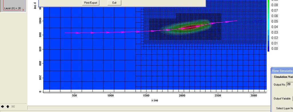
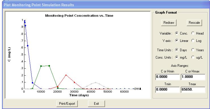
20 Figure 19 Step 6 View Solute Concentration Output and Monitoring Point Data Close the View Simulation Results dialog for hydraulic head output and on the main menu select Output > Solute Concentration to generate a plan-view flood map of the plume (Figure 20). By default the program initially selects an x-y slice through the highest concentration zone and the last simulation time (e.g., t = 50,000 days; z = 16.4 m in Figure 20). Zoom In to obtain the view in Figure 20. While in a plan or cross-section view, single click on any, or all, of the four monitoring point symbols to pop up a separate dialog containing graph(s) of the simulated concentration or hydraulic head versus time at these locations (Figures 20 and 21). 20

21 Figure 20 Figure 21 21

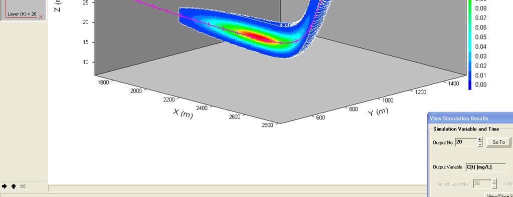
22 Step 7 Solute Concentration Cross-Section (x-z) View with Pathline To display the cross-sectional view in Figure 22, click on the X-Z Slice (Row) button in the lower left hand corner, and then select a row of cells (i.e., x-z slice; e.g., y = 979 m) that cuts through the plume (or select View > Change View Plane in the main menu). Zoom in to get a closer view of the plume. Figure 22 Step 8 3D Plume Volume Plot with Blanking As a final illustration, create a three-dimensional volume plot of the plume by selecting the 3D Volume radio button in the View Simulation Results dialog. Click on the Contour Options 22

23 button to load the Contour Parameters and Overlays dialog (Figure 23). Click on the Contour Options tab and change the concentration contour range to mg/l. Select the 3D Option tab in the Contour Parameters and Overlays dialog (Figure 23). Activate the first blanking parameter (click checkbox) and select C (mg/l) as the blanking parameter. Select the.le. operator and enter a value of mg/l to blank all cells with C.LE mg/l. Click the Redraw Contours button to view an isosurface of the central core of the plume. Now add a second blanking parameter to also view a slice through the plume. Click the + button and activate Y (m) (y-coordinate) as a blanking variable and enter y.le. 910 m. Click the - button to return to the first blanking variable (C) and select.or. as the logical operator. Click the Redraw Contours button to view a drawing similar to Figure 24. Note: the two blanking variables and logical operator are now: C.LE mg/l.or. y.le. 910 m Zoom in by increasing the Magnification to 4.0 and reduce the vertical exaggeration by increasing the Aspect Ratio to 3.0. Translate the drawing closer by changing the y Translation to -5. Click Redraw Contours. Finally, show the computed groundwater pathline (activate under the Pathlines tab) and the extraction well ( Overlays tab). You may also generate a higher resolution plot by changing to the High Graphics Resolution under the Contour Options tab (click Redraw Contours to generate). Figure 23 23

24 Figure 24 24