Computer Vision I - Algorithms and Applications: Image Formation Process Part 2
|
|
|
- Alban Ellis
- 6 years ago
- Views:
Transcription

1 Computer Vision I - Algorithms and Applications: Image Formation Process Part 2 Carsten Rother 17/11/2013 Computer Vision I: Image Formation Process
2 Computer Vision I: Image Formation Process 17/11/ Roadmap this lecture Geometric primitives and transformations (sec ) Geometric image formation (sec 2.1.5, 2.1.6) Pinhole camera Lens effects Photometric image formation process (sec 2.2) The Human eye Camera Types and Hardware (sec 2.3) Appearance based matching
3 Reminder: Pinhole Camera (Geometry) Computer Vision I: Image Formation Process 17/11/ Camera matrix P has 11 DoF Intrinsic parameters Principal point coordinates (p x, p y ) Focal length f Pixel magnification factors m Skew (non-rectangular pixels) s x = P X x = K R (I 3 3 C) ~ X K = f s p x 0 mf p y Extrinsic parameters ~ Rotation R (3DoF) and translation C (3DoF) relative to world coordinate system
4 Reminder: Lens effects Computer Vision I: Image Formation Process 17/11/2013 4
5 Computer Vision I: Image Formation Process 17/11/ Roadmap this lecture Geometric primitives and transformations (sec ) Geometric image formation (sec 2.1.5, 2.1.6) Pinhole camera Lens effects Photometric image formation process (sec 2.2) The Human eye Camera Types and Hardware (sec 2.3) Appearance based matching
6 Image formation Process Computer Vision I: Image Formation Process 17/11/2013 6
7 Model of the Surface Computer Vision I: Image Formation Process 17/11/ BRDF (Bi-diretcional Reflectance Function) light x ω i ω o Rendering equation: Outgoing energy (shining surface) Incoming light Outgoing energy: t time x position λ wavelength BRDF function (4DoF only ω i, ω o considered) ω i / ω o - incoming / outgoing direction Fore-shorting angle (always 0)

 Shading effects come from:")
8 Example: diffuse illumination Computer Vision I: Image Formation Process 17/11/ Rendering equation DIFFUSE 0 constant f r same for all ω o Single Light source: 0 constant constant (fixed ω i ) Shading effects come from: max(0, w i n)


9 Examples: BRDFs Computer Vision I: Image Formation Process 17/11/ Rendering equation (single light source) 0 constant (fixed ω i ) DIFFUSE SPECULAR DIFFUSE + ROUGH SPECULAR f r f r f r Single light source (top, right)

10 Inside a graphics engine Computer Vision I: Image Formation Process 17/11/ Rendering equation Ray tracing Radiosity


11 Example Computer Vision I: Image Formation Process 17/11/ Texture only 3D scene in blender Direct light Global (direct + indirect) light

12 How to model light? Computer Vision I: Image Formation Process 17/11/ Point light source Area light source Non-local illumination situation can be approximated with spherical harmonics First 9 spherical harmonics (gray scale) They can produce this


13 Capturig BRDF / BTF capture Computer Vision I: Image Formation Process 17/11/ BTF Bidirectional Texture function. At every spatial location x a different BRDF [Christopher Schwartz, Ralf Sarlette, Michael Weinmann and Reinhard Klein]

14 Fabricating BRDFs Computer Vision I: Image Formation Process 17/11/ [Levin et al. Siggraph 2013]

15 Single Image Computer Vision I: Image Formation Process 17/11/ [Barron and Malik 2012]

16 Single Image far from being solved Computer Vision I: Image Formation Process 17/11/ [Barron and Malik 2012]


17 Reconstruction and recognition Computer Vision I: Image Formation Process 17/11/ [Vinett, Rother, Torr, NIPS 13]
18 Computer Vision I: Image Formation Process 17/11/ Roadmap this lecture Geometric primitives and transformations (sec ) Geometric image formation (sec 2.1.5, 2.1.6) Pinhole camera Lens effects Photometric image formation process (sec 2.2) The Human eye Camera Types and Hardware (sec 2.3) Appearance based matching
.")
19 Computer Vision I: Image Formation Process 17/11/ The Human eye The retina contains different types of sensors: cones Zapfen (colors, 6 million) and rods Staebchen (gray levels, 120 million) The resolution is much higher In fovea centralis Light first passes through the layer of neurons before it reaches photo sensors (smoothing). Only in the fovea centralis the light hits directly the photo sensors Signal goes out the other way: Retina Ganglion cells (1 million) Optic nerve 1 MPixel Camera?
20 Spatial resolution Computer Vision I: Image Formation Process 17/11/

21 Spatial resolution 2MP Camera, far from the screen. Image Processing: Human seeing 5
22 Spatial resolution 5MP Camera, close to the screen. Image Processing: Human seeing 5
23 Spatial resolution (secrets) The resolution is much higher In fovea centralis The Information is pre-processed by Ganglion cells (Compare: =7MPixel, 2.4 MB RGB JPEG lossless) No still image, but a Video (super-resolution) Scanning technique Saccades Image Processing: Human seeing 8
 Saccades are driven by the importance of the scene parts (eyes,")
24 Eye Saccades Computer Vision I: Image Formation Process 17/11/ Eyes never move uniformly, but jump in saccades (approximately ms duration between fixation points) Saccades are driven by the importance of the scene parts (eyes, mouth etc).


25 The Human eye Computer Vision I: Image Formation Process 17/11/ cones Zapfen What is light? Spectrum, i.e. a function of the wavelength Different colors can be computed by adding /subtracting signal of rods Spectral resolution of the eye is relatively bad due to projection
26 Computer Vision I: Image Formation Process 17/11/ Roadmap this lecture Geometric primitives and transformations (sec ) Geometric image formation (sec 2.1.5, 2.1.6) Pinhole camera Lens effects Photometric image formation process (sec 2.2) The Human eye Camera Types and Hardware (sec 2.3) Appearance based matching
27 Camera types Computer Vision I: Image Formation Process 17/11/ RGB cameras Depth cameras: Passive RGB stereo Active Structured light Active Time of Flight Lightfield cameras
 Complementary metal oxide semiconductor")
28 Digital RGB cameras Computer Vision I: Image Formation Process 17/11/ A digital camera replaces film with a sensor array Each cell in the sensor array is light-sensitive diode that converts photons to electrons Two common types: Charge Coupled Device (CCD) Complementary metal oxide semiconductor (CMOS)

 See details on: http://www.dalsa.")
29 CCD versus CMOS Computer Vision I: Image Formation Process 17/11/ CCD: move charge from pixel to pixel and then converts to voltage and digital signal Negative: more expensive CMOS: converts to voltage inside the pixel Negative: slower to read out image ("rolling shutter" effect) See details on:

30 Color - Filters Computer Vision I: Image Formation Process 17/11/

31 Problem with de-mosaicing: color moiré Computer Vision I: Image Formation Process 17/11/

32 Cause of color moiré Computer Vision I: Image Formation Process 17/11/
 / noise")


33 General problems with RGB cameras Computer Vision I: Image Formation Process 17/11/ Noise low light is where you most notice noise light sensitivity (ISO) / noise tradeoff stuck pixels Resolution: Are more megapixels better? requires higher quality lens noise issues In-camera processing oversharpening can produce halos RAW vs. compressed file size vs. quality tradeoff Blooming charge overflowing into neighboring pixels More info online:


34 In-camera processing Computer Vision I: Image Formation Process 17/11/

35 Historical context of cameras Computer Vision I: Image Formation Process 17/11/
36 Camera types Computer Vision I: Image Formation Process 17/11/ RGB cameras Depth cameras: Passive RGB stereo Active Structured light Active Time of Flight Lightfield cameras


37 Passive Depth Camera RGB stereo Computer Vision I: Image Formation Process 17/11/ Easy to match hard to match

38 Active Depth Camera structured light Computer Vision I: Image Formation Process 17/11/ IR camera IR projector
 but now we have a very textured image Only works well when external IR light is not too string (not under")
39 Depth Camera structured light Computer Vision I: Image Formation Process 17/11/ Reference image from IR projector We have to perform matching (as with passive stereo camera) but now we have a very textured image Only works well when external IR light is not too string (not under sunlight)

40 Depth Camera structure Light Computer Vision I: Image Formation Process 17/11/
41 Halfway Computer Vision I: Image Formation Process 17/11/ Minutes Break Question?


42 Depth camera time of flight Computer Vision I: Image Formation Process 17/11/ Intensity image Depth Image PMD Camera
43 Principle Time of Flight Computer Vision I: Image Formation Process 17/11/ Modulated Light Source Cam Lens Sensor Pixel [slide credits: Rahul Nair, Daniel Kondermann]
44 Principle Time of Flight Computer Vision I: Image Formation Process 17/11/ Modulated Light Source Cam Lens Sensor Pixel [slide credits: Rahul Nair, Daniel Kondermann]
45 Principle Time of Flight Computer Vision I: Image Formation Process 17/11/ Modulated Light Source Cam Lens Sensor Pixel [slide credits: Rahul Nair, Daniel Kondermann]
46 Principle Time of Flight Computer Vision I: Image Formation Process 17/11/ Modulated Light Source Cam Lens Sensor Pixel [slide credits: Rahul Nair, Daniel Kondermann]
47 Principle Time of Flight Computer Vision I: Image Formation Process 17/11/ Modulated Light Source Cam Lens Sensor Pixel [slide credits: Rahul Nair, Daniel Kondermann]
48 Principle Time of Flight Computer Vision I: Image Formation Process 17/11/ Modulated Light Source Cam Lens Sensor Pixel [slide credits: Rahul Nair, Daniel Kondermann]
49 Principle Time of Flight Sensor Pixel Φ amplitude offset Measure: Phase shift Amplitude and offset Output: Depth Image (from phase shift) (wavelength determines the range of depth values; around 3.5 meter) 3.5meter Φ means d= 0.3m or 3.8m or 7.3m or (take differently modulated frequences) Intensity image (from amplitude and offset) [slide credits: Rahul Nair, Daniel Kondermann] Computer Vision I: Image Formation Process 17/11/

50 Depth camera time of flight Computer Vision I: Image Formation Process 17/11/ One of the biggest problems is multi-path


51 Lightfield cameras Computer Vision I: Image Formation Process 17/11/ Capture all light: Refocus and change perspective with one image
52 Computer Vision I: Image Formation Process 17/11/ Roadmap this lecture Geometric primitives and transformations (sec ) Geometric image formation (sec 2.1.5, 2.1.6) Pinhole camera Lens effects Photometric image formation process (sec 2.2) The Human eye Camera Types and Hardware (sec 2.3) Appearance based matching
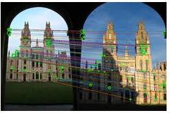
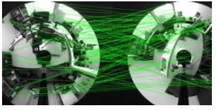
53 Roadmap: matching 2 Images (appearance & geometry) Computer Vision I: Image Formation Process 17/11/ Find interest points Find orientated patches around interest points to capture appearance Encode patch appearance in a descriptor Find matching patches according to appearance (similar descriptors) Verify matching patches according to geometry v
54 Roadmap: matching 2 Images (appearance & geometry) Computer Vision I: Image Formation Process 17/11/ Find interest points Find orientated patches around interest points to capture appearance Encode patch appearance in a descriptor Find matching patches according to appearance (similar descriptors) Verify matching patches according to geometry v

55 Reminder Lecture 3: Harris Corner Detector Computer Vision I: Image Formation Process 17/11/ Auto-correlation function: Harris measure:
56 Roadmap: matching 2 Images (appearance & geometry) Computer Vision I: Image Formation Process 17/11/ Find interest points Find orientated patches around interest points to capture appearance Encode patch appearance in a descriptor Find matching patches according to appearance (similar descriptors) Verify matching patches according to geometry v


57 How to deal with orientation Computer Vision I: Image Formation Process 17/11/ Orientate with image gradient:

58 Choose a patch around each point Computer Vision I: Image Formation Process 17/11/ How to deal with scale?

59 Choose a patch around each point Computer Vision I: Image Formation Process 17/11/ How to deal with scale?


60 Choose a patch around each point Computer Vision I: Image Formation Process 17/11/ How to deal with scale?
61 Scale selection (illustration) Computer Vision I: Image Formation Process 17/11/ f is Laplacian of Gaussian (LoG) operator. Measures an average edge-ness in all directions 2 G(σ) I = 2 (G(σ) I) x (G(σ) I) y 2 (details on page 191)
62 Scale selection (illustration) Computer Vision I: Image Formation Process 17/11/
63 Scale selection (illustration) Computer Vision I: Image Formation Process 17/11/

64 Scale selection (illustration) Computer Vision I: Image Formation Process 17/11/
65 Scale selection (illustration) Computer Vision I: Image Formation Process 17/11/ We could match-up these curves and find unique corresponding points
")


66 Scale selection (illustration) Computer Vision I: Image Formation Process 17/11/ Simpler: Find maxima /minima in image


67 Extensions: general affine transformations Computer Vision I: Image Formation Process 17/11/
68 Roadmap: matching 2 Images (appearance & geometry) Computer Vision I: Image Formation Process 17/11/ Find interest points Find orientated patches around interest points to capture appearance Encode patch appearance in a descriptor Find matching patches according to appearance (similar descriptors) Verify matching patches according to geometry v


69 SIFT feature 64 pixels Computer Vision I: Image Formation Process 17/11/ v 64 pixels 4*4=16 cells Each cell has an 8 bin histogram (smoothed across cells) In total: 16*8 values, i.e. 128D vector A cell has 16x16 pixels (here 8x8 for illustration only) (blue circle shows center weighting) [Lowe 2004]
 Can handle photometric changes (even day versus")
70 SIFT feature is very popular Computer Vision I: Image Formation Process 17/11/ Fast to compute Can handle large changes in viewpoint well (up to 60 o out of plane rotation) Can handle photometric changes (even day versus night)

71 Many other feature descriptors Computer Vision I: Image Formation Process 17/11/ MOPS [Brown, Szeliski and Winder 2005] SURF [Herbert Bay et al. 2006] DAISY [Tola, Lepetit, Fua 2010] Shape Context. DAISY
72 Roadmap: matching 2 Images (appearance & geometry) Computer Vision I: Image Formation Process 17/11/ Find interest points Find orientated patches around interest points to capture appearance Encode patch appearance in a descriptor Find matching patches according to appearance (similar descriptors) Verify matching patches according to geometry v
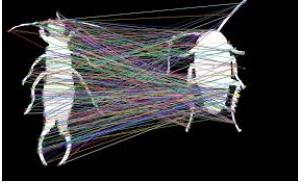
73 Appearance-based matching Computer Vision I: Image Formation Process 17/11/

74 Appearance-based matching Computer Vision I: Image Formation Process 17/11/ N patches (e.g. N = 1000) N patches (e.g. N = 1000) Goal: 1) Find for each patch in left image the closest in right image 2) Accept all matches where descriptors are similar enough Methods: Naïve: N 2 tests (here 1 Million) Hashing Hashing (locality sensitive hashing) Kd-tree; on average NlogN tests (here 10,000) (Hashing Function) Index for patch DB


75 Subtask: Search for one patch Computer Vision I: Image Formation Process 17/11/ Query patch? Database image


76 Nearest Neighbor Search Computer Vision I: Image Formation Process 17/11/ Tracking in Video The video is the Database Image retrieval Whole image has one descriptor Database is an image collection


 Example in 3D Result: balanced tree Nearest")
77 Kd-tree (d stands for dimension) Computer Vision I: Image Formation Process 17/11/ Build the tree over database image: 1) Cycle over dimensions: x,y,z,x,y,z,. 2) Put in axis-aligned hyper-planes (split at median of point set) Example in 3D Result: balanced tree Nearest Neighbour search (to come) [Invented by Jon Louis Bentley 1975]
78 Examples Computer Vision I: Image Formation Process 17/11/
79 Dimension 2 Examples Computer Vision I: Image Formation Process 17/11/ Kd-tree d1>5 2 1,2,3 4,5, Dimension 1
80 Dimension 2 Examples Computer Vision I: Image Formation Process 17/11/ Kd-tree d1>5 2 d2>4.8 d2> ,3 5 4, Dimension 1
81 Dimension 2 Examples Computer Vision I: Image Formation Process 17/11/ Kd-tree d1>5 2 d2>4.8 d2> d1>1 5 d1> Dimension
82 Dimension 2 Examples: nearest neighbor search Computer Vision I: Image Formation Process 17/11/ Kd-tree d1>5 2 d2>4.8 d2> query 1 d1>1 5 d1> Dimension
83 Dimension 2 Examples: nearest neighbor search Computer Vision I: Image Formation Process 17/11/ Kd-tree d1> search radius d2>4.8 d2>6.5 1 query 1 d1>1 5 d1> Dimension visited current best
84 Dimension 2 Examples: nearest neighbor search Computer Vision I: Image Formation Process 17/11/ Kd-tree d1>5 Radius not intersected search radius d2>4.8 d2>6.5 1 query 1 d1>1 5 d1> Dimension visited current best
85 Dimension 2 Examples: nearest neighbor search Computer Vision I: Image Formation Process 17/11/ Kd-tree Radius intersects so go down the subtree d1> search radius d2>4.8 d2>6.5 1 query 1 d1>1 5 d1> Dimension visited current best
86 Dimension 2 Examples: nearest neighbor search Computer Vision I: Image Formation Process 17/11/ Kd-tree d1> query search radius better solution found d2>4.8 d2>6.5 1 d1>1 5 d1> Dimension visited current best
87 Dimension 2 Examples: nearest neighbor search Computer Vision I: Image Formation Process 17/11/ Kd-tree d1> search radius d2>4.8 d2>6.5 1 query 1 d1>1 5 d1> Dimension 1 no need to visit these subtrees visited current best
88 Dimension 2 Examples: nearest neighbor search Computer Vision I: Image Formation Process 17/11/ Kd-tree d1> search radius d2>4.8 d2>6.5 1 query 1 d1>1 5 d1> Dimension Done since root-node is marked in both ways visited current best
89 Nearest neighbour search pseudo code Computer Vision I: Image Formation Process 17/11/ Input: query point Pseudo code Step 1: Find leave node (bucket) with query point Step 2: Make hyper-sphere with radius (current best and query point) Step3: go up the tree and see if hyper-plane intersects hyper-sphere Step 3a: no intersection: mark tree branch as visited since no better point can be found there. If node is root node then stop. Step 3b: intersection: go down the branch to find potentially a better point. If so, mark as current best and go to Step 2. Nothing better possible Hyper-plane positions Current best query On average O(log N)
90 Example with many points in 2D Computer Vision I: Image Formation Process 17/11/ From Andrew Moore:
91 Example with many points in 2D Computer Vision I: Image Formation Process 17/11/
92 Example with many points in 2D Computer Vision I: Image Formation Process 17/11/
93 Example with many points in 2D Computer Vision I: Image Formation Process 17/11/
94 Example with many points in 2D Computer Vision I: Image Formation Process 17/11/
95 Example with many points in 2D Computer Vision I: Image Formation Process 17/11/
96 Example with many points in 2D Computer Vision I: Image Formation Process 17/11/
97 Example with many points in 2D Computer Vision I: Image Formation Process 17/11/
98 Example with many points in 2D Computer Vision I: Image Formation Process 17/11/
99 Example with many points in 2D Computer Vision I: Image Formation Process 17/11/
100 Example with many points in 2D Computer Vision I: Image Formation Process 17/11/
101 Example with many points in 2D Computer Vision I: Image Formation Process 17/11/
102 Example with many points in 2D Computer Vision I: Image Formation Process 17/11/
103 Example with many points in 2D Computer Vision I: Image Formation Process 17/11/
104 Example with many points in 2D Computer Vision I: Image Formation Process 17/11/
105 Example with many points in 2D Computer Vision I: Image Formation Process 17/11/
106 Example with many points in 2D Computer Vision I: Image Formation Process 17/11/
107 Example with many points in 2D Computer Vision I: Image Formation Process 17/11/
108 Example with many points in 2D Computer Vision I: Image Formation Process 17/11/
109 Example with many points in 2D Computer Vision I: Image Formation Process 17/11/
110 Example with many points in 2D Computer Vision I: Image Formation Process 17/11/
111 Example with many points in 2D Computer Vision I: Image Formation Process 17/11/
112 Example with many points in 2D Computer Vision I: Image Formation Process 17/11/
113 Example with many points in 2D Computer Vision I: Image Formation Process 17/11/
114 Example with many points in 2D Computer Vision I: Image Formation Process 17/11/
115 Example with many points in 2D Computer Vision I: Image Formation Process 17/11/
116 Example with many points in 2D Computer Vision I: Image Formation Process 17/11/
117 Example with many points in 2D Computer Vision I: Image Formation Process 17/11/
118 Example with many points in 2D Computer Vision I: Image Formation Process 17/11/

119 Example with many points in 2D Computer Vision I: Image Formation Process 17/11/
120 Example with many points in 2D Computer Vision I: Image Formation Process 17/11/
121 Example with many points in 2D Computer Vision I: Image Formation Process 17/11/
122 Example with many points in 2D Computer Vision I: Image Formation Process 17/11/
123 Roadmap: matching 2 Images (appearance & geometry) Computer Vision I: Image Formation Process 17/11/ Find interest points (including different scales) Find orientated patches around interest points to capture appearance Encode patch in a descriptor Find matching patches according to appearance (similar descriptors) Verify matching patches according to geometry v
124 Reading for next class Computer Vision I: Basics of Image Processing 17/11/ This lecture: Photometric image formation (sec 2.2) Camera Types and Hardware (sec 2.3) Appearance matching: (sec ) Next lecture: Two-view Geometry (Hartley Zissermann)
Computer Vision I - Image Matching and Image Formation
 Computer Vision I - Image Matching and Image Formation Carsten Rother 10/12/2014 Computer Vision I: Image Formation Process Computer Vision I: Image Formation Process 10/12/2014 2 Roadmap for next five
Computer Vision I - Appearance-based Matching and Projective Geometry
 Computer Vision I - Appearance-based Matching and Projective Geometry Carsten Rother 01/11/2016 Computer Vision I: Image Formation Process Roadmap for next four lectures Computer Vision I: Image Formation
Computer Vision I - Appearance-based Matching and Projective Geometry
 Computer Vision I - Appearance-based Matching and Projective Geometry Carsten Rother 05/11/2015 Computer Vision I: Image Formation Process Roadmap for next four lectures Computer Vision I: Image Formation
Local features: detection and description. Local invariant features
 Local features: detection and description Local invariant features Detection of interest points Harris corner detection Scale invariant blob detection: LoG Description of local patches SIFT : Histograms
Outline 7/2/201011/6/
 Outline Pattern recognition in computer vision Background on the development of SIFT SIFT algorithm and some of its variations Computational considerations (SURF) Potential improvement Summary 01 2 Pattern
Local features and image matching. Prof. Xin Yang HUST
 Local features and image matching Prof. Xin Yang HUST Last time RANSAC for robust geometric transformation estimation Translation, Affine, Homography Image warping Given a 2D transformation T and a source
CS6670: Computer Vision
 CS6670: Computer Vision Noah Snavely Lecture 20: Light, reflectance and photometric stereo Light by Ted Adelson Readings Szeliski, 2.2, 2.3.2 Light by Ted Adelson Readings Szeliski, 2.2, 2.3.2 Properties
Geometric camera models and calibration
 Geometric camera models and calibration http://graphics.cs.cmu.edu/courses/15-463 15-463, 15-663, 15-862 Computational Photography Fall 2018, Lecture 13 Course announcements Homework 3 is out. - Due October
Range Sensors (time of flight) (1)
 (1)") Range Sensors (time of flight) (1) Large range distance measurement -> called range sensors Range information: key element for localization and environment modeling Ultrasonic sensors, infra-red sensors
Range Sensors (time of flight) (1) Large range distance measurement -> called range sensors Range information: key element for localization and environment modeling Ultrasonic sensors, infra-red sensors
Local Features: Detection, Description & Matching
 Local Features: Detection, Description & Matching Lecture 08 Computer Vision Material Citations Dr George Stockman Professor Emeritus, Michigan State University Dr David Lowe Professor, University of British
Automatic Image Alignment (feature-based)
") Automatic Image Alignment (feature-based) Mike Nese with a lot of slides stolen from Steve Seitz and Rick Szeliski 15-463: Computational Photography Alexei Efros, CMU, Fall 2006 Today s lecture Feature
Automatic Image Alignment (feature-based) Mike Nese with a lot of slides stolen from Steve Seitz and Rick Szeliski 15-463: Computational Photography Alexei Efros, CMU, Fall 2006 Today s lecture Feature
CS4670: Computer Vision
 CS4670: Computer Vision Noah Snavely Lecture 6: Feature matching and alignment Szeliski: Chapter 6.1 Reading Last time: Corners and blobs Scale-space blob detector: Example Feature descriptors We know
DD2423 Image Analysis and Computer Vision IMAGE FORMATION. Computational Vision and Active Perception School of Computer Science and Communication
 DD2423 Image Analysis and Computer Vision IMAGE FORMATION Mårten Björkman Computational Vision and Active Perception School of Computer Science and Communication November 8, 2013 1 Image formation Goal:
COSC579: Scene Geometry. Jeremy Bolton, PhD Assistant Teaching Professor
 COSC579: Scene Geometry Jeremy Bolton, PhD Assistant Teaching Professor Overview Linear Algebra Review Homogeneous vs non-homogeneous representations Projections and Transformations Scene Geometry The
Mosaics. Today s Readings
 Mosaics VR Seattle: http://www.vrseattle.com/ Full screen panoramas (cubic): http://www.panoramas.dk/ Mars: http://www.panoramas.dk/fullscreen3/f2_mars97.html Today s Readings Szeliski and Shum paper (sections
BSB663 Image Processing Pinar Duygulu. Slides are adapted from Selim Aksoy
 BSB663 Image Processing Pinar Duygulu Slides are adapted from Selim Aksoy Image matching Image matching is a fundamental aspect of many problems in computer vision. Object or scene recognition Solving
Image matching. Announcements. Harder case. Even harder case. Project 1 Out today Help session at the end of class. by Diva Sian.
 Announcements Project 1 Out today Help session at the end of class Image matching by Diva Sian by swashford Harder case Even harder case How the Afghan Girl was Identified by Her Iris Patterns Read the
Color and Shading. Color. Shapiro and Stockman, Chapter 6. Color and Machine Vision. Color and Perception
 Color and Shading Color Shapiro and Stockman, Chapter 6 Color is an important factor for for human perception for object and material identification, even time of day. Color perception depends upon both
The SIFT (Scale Invariant Feature
 The SIFT (Scale Invariant Feature Transform) Detector and Descriptor developed by David Lowe University of British Columbia Initial paper ICCV 1999 Newer journal paper IJCV 2004 Review: Matt Brown s Canonical
Local Feature Detectors
 Local Feature Detectors Selim Aksoy Department of Computer Engineering Bilkent University saksoy@cs.bilkent.edu.tr Slides adapted from Cordelia Schmid and David Lowe, CVPR 2003 Tutorial, Matthew Brown,
Harder case. Image matching. Even harder case. Harder still? by Diva Sian. by swashford
 Image matching Harder case by Diva Sian by Diva Sian by scgbt by swashford Even harder case Harder still? How the Afghan Girl was Identified by Her Iris Patterns Read the story NASA Mars Rover images Answer
CS5670: Computer Vision
 CS5670: Computer Vision Noah Snavely Light & Perception Announcements Quiz on Tuesday Project 3 code due Monday, April 17, by 11:59pm artifact due Wednesday, April 19, by 11:59pm Can we determine shape
CS 4495 Computer Vision A. Bobick. CS 4495 Computer Vision. Features 2 SIFT descriptor. Aaron Bobick School of Interactive Computing
 CS 4495 Computer Vision Features 2 SIFT descriptor Aaron Bobick School of Interactive Computing Administrivia PS 3: Out due Oct 6 th. Features recap: Goal is to find corresponding locations in two images.
Local features: detection and description May 12 th, 2015
 Local features: detection and description May 12 th, 2015 Yong Jae Lee UC Davis Announcements PS1 grades up on SmartSite PS1 stats: Mean: 83.26 Standard Dev: 28.51 PS2 deadline extended to Saturday, 11:59
3D graphics, raster and colors CS312 Fall 2010
 Computer Graphics 3D graphics, raster and colors CS312 Fall 2010 Shift in CG Application Markets 1989-2000 2000 1989 3D Graphics Object description 3D graphics model Visualization 2D projection that simulates
Harder case. Image matching. Even harder case. Harder still? by Diva Sian. by swashford
 Image matching Harder case by Diva Sian by Diva Sian by scgbt by swashford Even harder case Harder still? How the Afghan Girl was Identified by Her Iris Patterns Read the story NASA Mars Rover images Answer
10/5/09 1. d = 2. Range Sensors (time of flight) (2) Ultrasonic Sensor (time of flight, sound) (1) Ultrasonic Sensor (time of flight, sound) (2) 4.1.
 (2) Ultrasonic Sensor (time of flight, sound) (1) Ultrasonic Sensor (time of flight, sound) (2) 4.1.") Range Sensors (time of flight) (1) Range Sensors (time of flight) (2) arge range distance measurement -> called range sensors Range information: key element for localization and environment modeling Ultrasonic
Range Sensors (time of flight) (1) Range Sensors (time of flight) (2) arge range distance measurement -> called range sensors Range information: key element for localization and environment modeling Ultrasonic
Representing the World
 Table of Contents Representing the World...1 Sensory Transducers...1 The Lateral Geniculate Nucleus (LGN)... 2 Areas V1 to V5 the Visual Cortex... 2 Computer Vision... 3 Intensity Images... 3 Image Focusing...
Computer Vision for HCI. Topics of This Lecture
 Computer Vision for HCI Interest Points Topics of This Lecture Local Invariant Features Motivation Requirements, Invariances Keypoint Localization Features from Accelerated Segment Test (FAST) Harris Shi-Tomasi
Computer Vision Course Lecture 02. Image Formation Light and Color. Ceyhun Burak Akgül, PhD cba-research.com. Spring 2015 Last updated 04/03/2015
 Computer Vision Course Lecture 02 Image Formation Light and Color Ceyhun Burak Akgül, PhD cba-research.com Spring 2015 Last updated 04/03/2015 Photo credit: Olivier Teboul vision.mas.ecp.fr/personnel/teboul
Topics and things to know about them:
 Practice Final CMSC 427 Distributed Tuesday, December 11, 2007 Review Session, Monday, December 17, 5:00pm, 4424 AV Williams Final: 10:30 AM Wednesday, December 19, 2007 General Guidelines: The final will
Miniature faking. In close-up photo, the depth of field is limited.
 Miniature faking In close-up photo, the depth of field is limited. http://en.wikipedia.org/wiki/file:jodhpur_tilt_shift.jpg Miniature faking Miniature faking http://en.wikipedia.org/wiki/file:oregon_state_beavers_tilt-shift_miniature_greg_keene.jpg
Light. Computer Vision. James Hays
 Light Computer Vision James Hays Projection: world coordinatesimage coordinates Camera Center (,, ) z y x X... f z y ' ' v u x. v u z f x u * ' z f y v * ' 5 2 ' 2* u 5 2 ' 3* v If X = 2, Y = 3, Z = 5,
Image Formation: Light and Shading. Introduction to Computer Vision CSE 152 Lecture 3
 Image Formation: Light and Shading CSE 152 Lecture 3 Announcements Homework 1 is due Apr 11, 11:59 PM Homework 2 will be assigned on Apr 11 Reading: Chapter 2: Light and Shading Geometric image formation
Scale Invariant Feature Transform
 Scale Invariant Feature Transform Why do we care about matching features? Camera calibration Stereo Tracking/SFM Image moiaicing Object/activity Recognition Objection representation and recognition Image
HISTOGRAMS OF ORIENTATIO N GRADIENTS
 HISTOGRAMS OF ORIENTATIO N GRADIENTS Histograms of Orientation Gradients Objective: object recognition Basic idea Local shape information often well described by the distribution of intensity gradients
Digital Image Processing COSC 6380/4393
 Digital Image Processing COSC 6380/4393 Lecture 21 Nov 16 th, 2017 Pranav Mantini Ack: Shah. M Image Processing Geometric Transformation Point Operations Filtering (spatial, Frequency) Input Restoration/
Feature Based Registration - Image Alignment
 Feature Based Registration - Image Alignment Image Registration Image registration is the process of estimating an optimal transformation between two or more images. Many slides from Alexei Efros http://graphics.cs.cmu.edu/courses/15-463/2007_fall/463.html
Laser sensors. Transmitter. Receiver. Basilio Bona ROBOTICA 03CFIOR
 Mobile & Service Robotics Sensors for Robotics 3 Laser sensors Rays are transmitted and received coaxially The target is illuminated by collimated rays The receiver measures the time of flight (back and
CS201 Computer Vision Lect 4 - Image Formation
 CS201 Computer Vision Lect 4 - Image Formation John Magee 9 September, 2014 Slides courtesy of Diane H. Theriault Question of the Day: Why is Computer Vision hard? Something to think about from our view
Midterm Exam CS 184: Foundations of Computer Graphics page 1 of 11
 Midterm Exam CS 184: Foundations of Computer Graphics page 1 of 11 Student Name: Class Account Username: Instructions: Read them carefully! The exam begins at 2:40pm and ends at 4:00pm. You must turn your
Multiple-Choice Questionnaire Group C
 Family name: Vision and Machine-Learning Given name: 1/28/2011 Multiple-Choice naire Group C No documents authorized. There can be several right answers to a question. Marking-scheme: 2 points if all right
Chapter 32 Light: Reflection and Refraction. Copyright 2009 Pearson Education, Inc.
 Chapter 32 Light: Reflection and Refraction Units of Chapter 32 The Ray Model of Light Reflection; Image Formation by a Plane Mirror Formation of Images by Spherical Mirrors Index of Refraction Refraction:
Lenses: Focus and Defocus
 Lenses: Focus and Defocus circle of confusion A lens focuses light onto the film There is a specific distance at which objects are in focus other points project to a circle of confusion in the image Changing
All good things must...
 Lecture 17 Final Review All good things must... UW CSE vision faculty Course Grading Programming Projects (80%) Image scissors (20%) -DONE! Panoramas (20%) - DONE! Content-based image retrieval (20%) -
Image correspondences and structure from motion
 Image correspondences and structure from motion http://graphics.cs.cmu.edu/courses/15-463 15-463, 15-663, 15-862 Computational Photography Fall 2017, Lecture 20 Course announcements Homework 5 posted.
Scale Invariant Feature Transform
 Why do we care about matching features? Scale Invariant Feature Transform Camera calibration Stereo Tracking/SFM Image moiaicing Object/activity Recognition Objection representation and recognition Automatic
Chapter 2 - Fundamentals. Comunicação Visual Interactiva
 Chapter - Fundamentals Comunicação Visual Interactiva Structure of the human eye (1) CVI Structure of the human eye () Celular structure of the retina. On the right we can see one cone between two groups
Motion illusion, rotating snakes
 Motion illusion, rotating snakes Local features: main components 1) Detection: Find a set of distinctive key points. 2) Description: Extract feature descriptor around each interest point as vector. x 1
Feature descriptors and matching
 Feature descriptors and matching Detections at multiple scales Invariance of MOPS Intensity Scale Rotation Color and Lighting Out-of-plane rotation Out-of-plane rotation Better representation than color:
EXAM SOLUTIONS. Computer Vision Course 2D1420 Thursday, 11 th of march 2003,
 Numerical Analysis and Computer Science, KTH Danica Kragic EXAM SOLUTIONS Computer Vision Course 2D1420 Thursday, 11 th of march 2003, 8.00 13.00 Exercise 1 (5*2=10 credits) Answer at most 5 of the following
Midterm Examination CS 534: Computational Photography
 Midterm Examination CS 534: Computational Photography November 3, 2016 NAME: Problem Score Max Score 1 6 2 8 3 9 4 12 5 4 6 13 7 7 8 6 9 9 10 6 11 14 12 6 Total 100 1 of 8 1. [6] (a) [3] What camera setting(s)
Announcements. Image Formation: Light and Shading. Photometric image formation. Geometric image formation
 Announcements Image Formation: Light and Shading Homework 0 is due Oct 5, 11:59 PM Homework 1 will be assigned on Oct 5 Reading: Chapters 2: Light and Shading CSE 252A Lecture 3 Geometric image formation
Computer Vision. The image formation process
 Computer Vision The image formation process Filippo Bergamasco (filippo.bergamasco@unive.it) http://www.dais.unive.it/~bergamasco DAIS, Ca Foscari University of Venice Academic year 2016/2017 The image
Midterm Wed. Local features: detection and description. Today. Last time. Local features: main components. Goal: interest operator repeatability
 Midterm Wed. Local features: detection and description Monday March 7 Prof. UT Austin Covers material up until 3/1 Solutions to practice eam handed out today Bring a 8.5 11 sheet of notes if you want Review
Outline. ETN-FPI Training School on Plenoptic Sensing
 Outline Introduction Part I: Basics of Mathematical Optimization Linear Least Squares Nonlinear Optimization Part II: Basics of Computer Vision Camera Model Multi-Camera Model Multi-Camera Calibration
CS6670: Computer Vision
 CS6670: Computer Vision Noah Snavely Lecture 21: Light, reflectance and photometric stereo Announcements Final projects Midterm reports due November 24 (next Tuesday) by 11:59pm (upload to CMS) State the
Game Programming. Bing-Yu Chen National Taiwan University
 Game Programming Bing-Yu Chen National Taiwan University What is Computer Graphics? Definition the pictorial synthesis of real or imaginary objects from their computer-based models descriptions OUTPUT
Stereo Vision. MAN-522 Computer Vision
 Stereo Vision MAN-522 Computer Vision What is the goal of stereo vision? The recovery of the 3D structure of a scene using two or more images of the 3D scene, each acquired from a different viewpoint in
Image Features. Work on project 1. All is Vanity, by C. Allan Gilbert,
 Image Features Work on project 1 All is Vanity, by C. Allan Gilbert, 1873-1929 Feature extrac*on: Corners and blobs c Mo*va*on: Automa*c panoramas Credit: Ma9 Brown Why extract features? Mo*va*on: panorama
Computer Graphics. Bing-Yu Chen National Taiwan University The University of Tokyo
 Computer Graphics Bing-Yu Chen National Taiwan University The University of Tokyo Introduction The Graphics Process Color Models Triangle Meshes The Rendering Pipeline 1 What is Computer Graphics? modeling
Feature Detection. Raul Queiroz Feitosa. 3/30/2017 Feature Detection 1
 Feature Detection Raul Queiroz Feitosa 3/30/2017 Feature Detection 1 Objetive This chapter discusses the correspondence problem and presents approaches to solve it. 3/30/2017 Feature Detection 2 Outline
Project 4 Results. Representation. Data. Learning. Zachary, Hung-I, Paul, Emanuel. SIFT and HoG are popular and successful.
 Project 4 Results Representation SIFT and HoG are popular and successful. Data Hugely varying results from hard mining. Learning Non-linear classifier usually better. Zachary, Hung-I, Paul, Emanuel Project
EECS150 - Digital Design Lecture 14 FIFO 2 and SIFT. Recap and Outline
 EECS150 - Digital Design Lecture 14 FIFO 2 and SIFT Oct. 15, 2013 Prof. Ronald Fearing Electrical Engineering and Computer Sciences University of California, Berkeley (slides courtesy of Prof. John Wawrzynek)
Rendering: Reality. Eye acts as pinhole camera. Photons from light hit objects
 Basic Ray Tracing Rendering: Reality Eye acts as pinhole camera Photons from light hit objects Rendering: Reality Eye acts as pinhole camera Photons from light hit objects Rendering: Reality Eye acts as
Local invariant features
 Local invariant features Tuesday, Oct 28 Kristen Grauman UT-Austin Today Some more Pset 2 results Pset 2 returned, pick up solutions Pset 3 is posted, due 11/11 Local invariant features Detection of interest
Automatic Image Alignment
 Automatic Image Alignment with a lot of slides stolen from Steve Seitz and Rick Szeliski Mike Nese CS194: Image Manipulation & Computational Photography Alexei Efros, UC Berkeley, Fall 2018 Live Homography
Other approaches to obtaining 3D structure
 Other approaches to obtaining 3D structure Active stereo with structured light Project structured light patterns onto the object simplifies the correspondence problem Allows us to use only one camera camera
The exam begins at 2:40pm and ends at 4:00pm. You must turn your exam in when time is announced or risk not having it accepted.
 CS 184: Foundations of Computer Graphics page 1 of 10 Student Name: Class Account Username: Instructions: Read them carefully! The exam begins at 2:40pm and ends at 4:00pm. You must turn your exam in when
Information page for written examinations at Linköping University TER2
 Information page for written examinations at Linköping University Examination date 2016-08-19 Room (1) TER2 Time 8-12 Course code Exam code Course name Exam name Department Number of questions in the examination
Light. Properties of light. What is light? Today What is light? How do we measure it? How does light propagate? How does light interact with matter?
 Light Properties of light Today What is light? How do we measure it? How does light propagate? How does light interact with matter? by Ted Adelson Readings Andrew Glassner, Principles of Digital Image
Computer Vision I - Filtering and Feature detection
 Computer Vision I - Filtering and Feature detection Carsten Rother 30/10/2015 Computer Vision I: Basics of Image Processing Roadmap: Basics of Digital Image Processing Computer Vision I: Basics of Image
Radiometry and reflectance
 Radiometry and reflectance http://graphics.cs.cmu.edu/courses/15-463 15-463, 15-663, 15-862 Computational Photography Fall 2018, Lecture 16 Course announcements Homework 4 is still ongoing - Any questions?
Reflectance & Lighting
 Reflectance & Lighting Computer Vision I CSE5A Lecture 6 Last lecture in a nutshell Need for lenses (blur from pinhole) Thin lens equation Distortion and aberrations Vignetting CS5A, Winter 007 Computer
Complex Sensors: Cameras, Visual Sensing. The Robotics Primer (Ch. 9) ECE 497: Introduction to Mobile Robotics -Visual Sensors
 ECE 497: Introduction to Mobile Robotics -Visual Sensors") Complex Sensors: Cameras, Visual Sensing The Robotics Primer (Ch. 9) Bring your laptop and robot everyday DO NOT unplug the network cables from the desktop computers or the walls Tuesday s Quiz is on Visual
Complex Sensors: Cameras, Visual Sensing The Robotics Primer (Ch. 9) Bring your laptop and robot everyday DO NOT unplug the network cables from the desktop computers or the walls Tuesday s Quiz is on Visual
CAP 5415 Computer Vision Fall 2012
 CAP 5415 Computer Vision Fall 01 Dr. Mubarak Shah Univ. of Central Florida Office 47-F HEC Lecture-5 SIFT: David Lowe, UBC SIFT - Key Point Extraction Stands for scale invariant feature transform Patented
CS4495/6495 Introduction to Computer Vision
 CS4495/6495 Introduction to Computer Vision 9C-L1 3D perception Some slides by Kelsey Hawkins Motivation Why do animals, people & robots need vision? To detect and recognize objects/landmarks Is that a
Contents I IMAGE FORMATION 1
 Contents I IMAGE FORMATION 1 1 Geometric Camera Models 3 1.1 Image Formation............................. 4 1.1.1 Pinhole Perspective....................... 4 1.1.2 Weak Perspective.........................
Advanced Graphics. Path Tracing and Photon Mapping Part 2. Path Tracing and Photon Mapping
 Advanced Graphics Path Tracing and Photon Mapping Part 2 Path Tracing and Photon Mapping Importance Sampling Combine importance sampling techniques Reflectance function (diffuse + specular) Light source
Computer Vision. Recap: Smoothing with a Gaussian. Recap: Effect of σ on derivatives. Computer Science Tripos Part II. Dr Christopher Town
 Recap: Smoothing with a Gaussian Computer Vision Computer Science Tripos Part II Dr Christopher Town Recall: parameter σ is the scale / width / spread of the Gaussian kernel, and controls the amount of
CEE598 - Visual Sensing for Civil Infrastructure Eng. & Mgmt.
 CEE598 - Visual Sensing for Civil Infrastructure Eng. & Mgmt. Section 10 - Detectors part II Descriptors Mani Golparvar-Fard Department of Civil and Environmental Engineering 3129D, Newmark Civil Engineering
Part I The Basic Algorithm. Principles of Photon Mapping. A two-pass global illumination method Pass I Computing the photon map
 Part I The Basic Algorithm 1 Principles of A two-pass global illumination method Pass I Computing the photon map A rough representation of the lighting in the scene Pass II rendering Regular (distributed)
Computer and Machine Vision
 Computer and Machine Vision Lecture Week 12 Part-2 Additional 3D Scene Considerations March 29, 2014 Sam Siewert Outline of Week 12 Computer Vision APIs and Languages Alternatives to C++ and OpenCV API
Image Formation. Antonino Furnari. Image Processing Lab Dipartimento di Matematica e Informatica Università degli Studi di Catania
 Image Formation Antonino Furnari Image Processing Lab Dipartimento di Matematica e Informatica Università degli Studi di Catania furnari@dmi.unict.it 18/03/2014 Outline Introduction; Geometric Primitives
Camera Calibration. Schedule. Jesus J Caban. Note: You have until next Monday to let me know. ! Today:! Camera calibration
 Camera Calibration Jesus J Caban Schedule! Today:! Camera calibration! Wednesday:! Lecture: Motion & Optical Flow! Monday:! Lecture: Medical Imaging! Final presentations:! Nov 29 th : W. Griffin! Dec 1
INFOGR Computer Graphics. J. Bikker - April-July Lecture 10: Shading Models. Welcome!
 INFOGR Computer Graphics J. Bikker - April-July 2016 - Lecture 10: Shading Models Welcome! Today s Agenda: Introduction Light Transport Materials Sensors Shading INFOGR Lecture 10 Shading Models 3 Introduction
Range Imaging Through Triangulation. Range Imaging Through Triangulation. Range Imaging Through Triangulation. Range Imaging Through Triangulation
 Obviously, this is a very slow process and not suitable for dynamic scenes. To speed things up, we can use a laser that projects a vertical line of light onto the scene. This laser rotates around its vertical
All human beings desire to know. [...] sight, more than any other senses, gives us knowledge of things and clarifies many differences among them.
![All human beings desire to know. [...] sight, more than any other senses, gives us knowledge of things and clarifies many differences among them.](/thumbs/91/106597332.jpg "All human beings desire to know. [...] sight, more than any other senses, gives us knowledge of things and clarifies many differences among them.") All human beings desire to know. [...] sight, more than any other senses, gives us knowledge of things and clarifies many differences among them. - Aristotle University of Texas at Arlington Introduction
All human beings desire to know. [...] sight, more than any other senses, gives us knowledge of things and clarifies many differences among them. - Aristotle University of Texas at Arlington Introduction
Jingyi Yu CISC 849. Department of Computer and Information Science
 Digital Photography and Videos Jingyi Yu CISC 849 Light Fields, Lumigraph, and Image-based Rendering Pinhole Camera A camera captures a set of rays A pinhole camera captures a set of rays passing through
Object Recognition with Invariant Features
 Object Recognition with Invariant Features Definition: Identify objects or scenes and determine their pose and model parameters Applications Industrial automation and inspection Mobile robots, toys, user
Automatic Image Alignment
 Automatic Image Alignment Mike Nese with a lot of slides stolen from Steve Seitz and Rick Szeliski 15-463: Computational Photography Alexei Efros, CMU, Fall 2010 Live Homography DEMO Check out panoramio.com
Midterm Exam! CS 184: Foundations of Computer Graphics! page 1 of 13!
 Midterm Exam! CS 184: Foundations of Computer Graphics! page 1 of 13! Student Name:!! Class Account Username:! Instructions: Read them carefully!! The exam begins at 1:10pm and ends at 2:30pm. You must
Building a Panorama. Matching features. Matching with Features. How do we build a panorama? Computational Photography, 6.882
 Matching features Building a Panorama Computational Photography, 6.88 Prof. Bill Freeman April 11, 006 Image and shape descriptors: Harris corner detectors and SIFT features. Suggested readings: Mikolajczyk
Computer Graphics. - Ray Tracing I - Marcus Magnor Philipp Slusallek. Computer Graphics WS05/06 Ray Tracing I
 Computer Graphics - Ray Tracing I - Marcus Magnor Philipp Slusallek Overview Last Lecture Introduction Today Ray tracing I Background Basic ray tracing What is possible? Recursive ray tracing algorithm
Dense 3D Reconstruction. Christiano Gava
 Dense 3D Reconstruction Christiano Gava christiano.gava@dfki.de Outline Previous lecture: structure and motion II Structure and motion loop Triangulation Today: dense 3D reconstruction The matching problem
Assignment #2. (Due date: 11/6/2012)
") Computer Vision I CSE 252a, Fall 2012 David Kriegman Assignment #2 (Due date: 11/6/2012) Name: Student ID: Email: Problem 1 [1 pts] Calculate the number of steradians contained in a spherical wedge with
Computer Vision I CSE 252a, Fall 2012 David Kriegman Assignment #2 (Due date: 11/6/2012) Name: Student ID: Email: Problem 1 [1 pts] Calculate the number of steradians contained in a spherical wedge with
SIFT - scale-invariant feature transform Konrad Schindler
 SIFT - scale-invariant feature transform Konrad Schindler Institute of Geodesy and Photogrammetry Invariant interest points Goal match points between images with very different scale, orientation, projective
Cameras and Stereo CSE 455. Linda Shapiro
 Cameras and Stereo CSE 455 Linda Shapiro 1 Müller-Lyer Illusion http://www.michaelbach.de/ot/sze_muelue/index.html What do you know about perspective projection? Vertical lines? Other lines? 2 Image formation
SIFT: SCALE INVARIANT FEATURE TRANSFORM SURF: SPEEDED UP ROBUST FEATURES BASHAR ALSADIK EOS DEPT. TOPMAP M13 3D GEOINFORMATION FROM IMAGES 2014
 SIFT: SCALE INVARIANT FEATURE TRANSFORM SURF: SPEEDED UP ROBUST FEATURES BASHAR ALSADIK EOS DEPT. TOPMAP M13 3D GEOINFORMATION FROM IMAGES 2014 SIFT SIFT: Scale Invariant Feature Transform; transform image
Lecture 19: Depth Cameras. Visual Computing Systems CMU , Fall 2013
 Lecture 19: Depth Cameras Visual Computing Systems Continuing theme: computational photography Cameras capture light, then extensive processing produces the desired image Today: - Capturing scene depth