Reconstructing a Fragmented Face from an Attacked Secure Identification Protocol

Transcription

1 Reconstructing a Fragmented Face from an Attacked Secure Identification Protocol Andy Luong Supervised by Professor Kristen Grauman Department of Computer Science University of Texas at Austin aluong@cs.utexas.edu May 6, 2011

2 Abstract Secure facial identification systems compare an input face to a protected list of subjects. If this list were to be made public, there would be a severe privacy/confidentiality breach. A common approach to protect these lists of faces is to store a representation (descriptor or vector) of the face that is not directly mappable to its original form. In this thesis, we consider a recently developed secure identification system, Secure Computation of Face Identification (SCiFI) [1], that utilizes an index-based facial vector to discretely compress the representation of a face image. A facial descriptor of this system does not allow for a complete reverse mapping. However, we show that if a malicious user is able to obtain a facial descriptor, it is possible that he/she can reconstruct an identifiable human face. We develop a novel approach to initially assemble the information given by the SCiFI protocol to create a fragmented face. This image has large missing regions due to SCiFI s facial representation. Thus, we estimate the missing regions of the face using an iterative Principal Component Analysis (PCA) technique. This is done by first building a face subspace based on a public set of human faces. Then, given the assembled image from the SCiFI protocol, we iteratively project this image in and out of the subspace to obtain a complete human face. Traditionally, PCA reconstruction techniques have been used to estimate very small or specific occluded regions of a face image; these techniques have also been used in facial recognition such as through a k-nearest neighbor approach. However, in our new method, we use it to synthesize 60% to 80% of a human face for facial identification. We explore novel methods of comparing images from different subspaces using metric learning and other forms of facial descriptors. We test our reconstruction with face identification tasks given to a human and a computer. Our results show that our reconstructions are consistently more informative than what is extracted from the SCiFI facial descriptor alone. In addition, these tasks show that our reconstructions are identifiable by humans and computers. The success of our approach implies that a malicious attacker could expose the faces on a registered database.

3 Contents 1 Introduction 4 2 Related Work Modeling Human Faces Secure Facial Recognition Reconstructing Occluded Regions of Faces The Secure Computation of Face Identification (SCiFI) System Overview Face Representation Comparing Faces High-Level SCiFI Protocol Cryptographic Attack Approach Offline Processing Face Part Vocabulary Constructing a Face Subspace Online Facial Reconstruction Finding Best Matching Patches Principal Component Analysis - Based Face Reconstruction Experiments and Results Databases PUT Face Facetracer Methodology Implementation Details Experimental Results Qualitative Results Quantifying Reconstruction Error Machine Face Recognition Experiment Human Experiment Discussion 48 1

4 7 Conclusion 50 2

5 List of Figures 1.1 Airport Facial Identification Application SCiFI Facial Reconstruction Workflow SCiFI Facial Vector Diagram SCiFI Overview Offline Processing Extraction of Appearance and Spatial Words Examples of Appearance Vocabulary Clustering Distance Measure Comparisons Affine Transformation Online Processing Overview Patch Face Illustration Iterative PCA Face Reconstruction Recursive PCA Reconstruction Iterations Approach Summary PUT and Facetracer Faces PUT Dataset Examples Facetracer Dataset Examples Datasets Appearance Vocabularies Facetracer - Male and Female Reconstruction Examples Facetracer - Male or Female Reconstruction Examples PUT Reconstruction Examples Quantifying Reconstruction Overview Quantifying Reconstruction Quality Boxplots Machine Face Recognition Overview Machine Face Recognition Plots SCiFI Test Screenshot Human Experiments Results Human Test Results Table Example of Human Test Reconstructions

6 Chapter 1 Introduction A large research area in computer vision is focused around facial recognition and detection. This area of study has great applications in security, as we can use facial recognition as a form of biometric identification. An identification task is where a system compares a single image with a list of stored images and determines if there is a close match. This process is especially useful in surveillance for identifying terrorists, criminals, or missing people from a single shot of their face. A simple facial recognition system can be implemented to perform this task. For example, Figure 1.1 outlines an application where facial identification is useful in an airport. Airport authorities can use this system to screen dangerous personnel from being able to board their planes. An identification system would screen passengers by checking if their faces are listed in a suspect or no-fly list stored on an external server. The security camera takes images of passengers and cross-examines them with a suspect list stored on the server. Only the server is aware of a match and it can then notify airport authorities. The caveat of this system is that the public often believes surveillance cameras or videos are a violation of privacy. Most people do not want their day to day activities being recorded. In addition, a compromised system could be used to link faces with identities through social networking sites or any form of a profile database. Thus, an appropriate response would be to implement cryptography in the system and have data encrypted. Even though people are still being recorded, encryption will protect the confidentiality of the individuals. However, by introducing cryptography, scalability and efficiency are an immediate problem. Images can be very large depending on their resolution and converting a continuous comparison of a face to a discrete measure for a cryptographic algorithm will affect facial recognition accuracy. Consequently, it is not a trivial task to integrate both of these ideas together. The Secure Computation of Face Identification (SCiFI) [1] is a recently developed system that attempts to combine security with facial recognition. It performs facial identification while providing secure transmissions and facial comparisons. SCiFI allows two mutually untrusting parties to represent and compare facial images efficiently and securely. The SCiFI system s protocol performs a cross-reference of faces, while not providing any additional information about who is being compared or what individuals are in the database. Consequently, the suspect list is confidential and input faces in the system are only used to check for matches. If a hacker or eavesdropper is able to see the system queries or obtain the 4

7 Figure 1.1: Data flow for an identification system; e.g. at an airport. Passenger faces are initially captured by a security camera as passengers pass through the security checkpoint. The security camera transmits each face to the server to be compared. If the server sees a match with any faces in its database, it notifies airport security. suspect database, he/she would not be able to directly retrieve actual faces of people. By design, face images are not stored directly in the SCiFI system. Rather, each face is decomposed and then represented by a bit vector formed from an index-based model. This model is built from a completely external public set of faces. The facial vector is a binary encoding of facial part appearances and their relative spatial distances. When comparing two faces, the Hamming distance is computed between them. If the distance does not exceed a certain threshold, the faces are a match. The public faces are independent of the suspect faces; therefore, at most, an attacker that is able to break the cryptographic protocol, could gain information about parts that are similar to a suspect s face. This is why reconstructing a human face is not trivial under SCiFI. Consequently, one may ask, Does that mean SCiFI has completely addressed the privacy concern mentioned earlier? We will actually show that the privacy threat does not end here. In fact, the problem addressed in my thesis is how a malicious party can use the learned facial vectors to expose the faces of the subjects stored on the server or sent by the client. Recall that the SCiFI system discards the true image of the person when it constructs the facial vector. In addition, the facial part appearances, indexed by the face vector, only provide information about 30% of the face; roughly 60%-80% of the actual face is never represented. The 30% of the face that is represented is also not humanly recognizable, because it s a collection of other people s facial parts. Thus, reconstructing a humanly identifiable face requires more work than merely breaking the secure protocol. However, we will show that this task is not impossible. In particular, we will describe a reconstruction algorithm that will result in a police sketch quality image that resembles the original face. However, our reconstruction is useless, unless facial vectors can be obtained. It can be 5

8 shown that the SCiFI system is not secure should one of the parties acts arbitrarily [2]. By submitting a series of ill-formed vectors, an attacker can retrieve an entire facial vector from the database or learn the client s input facial vector. The basic premise of the attack is that the malicious party sends facial vectors with only certain bits set to the server and analyzes their Hamming distances. Slowly, the malicious party can learn bit-by-bit the facial vector stored on the server or sent by the client. This attack is possible because the protocol does not distinguish between well-formed facial vectors (from actual faces) and arbitrary vectors. It is important to point out that with merely the cryptographic attack, the facial vector does not provide enough information to learn the original person s face. It requires an additional facial reconstruction step to obtain recognizable faces. In this thesis, I introduce an approach to reconstruct a human face from a facial vector of an attacked SCiFI protocol. The main idea of this approach is to assemble a fragmented face from SCiFI s facial representation, and then use this image as the base image for hallucinating and reconstructing a human face using a PCA technique. The proposed reconstruction technique can be divided into two stages. The first stage is done offline and is mainly preprocessing of the public database of faces used to build the SCiFI facial representations. The second stage is the actual facial reconstruction process and is done online after obtaining the facial vector. During the online stage, the first step of reconstruction is to retrieve the corresponding parts and spatial values from the actual public database identified in the facial vector. This is done by examining the facial vector and locating which bits are set. The next step is to construct a fragmented patch face, which combines the indexed patches of facial features and spatial distances from the public database. At this step, the attacker has an image that loosely resembles a human face. However, since different parts from different faces are assembled in the image, it is very difficult to identify any individual. The faces will look very abstract at the end of this procedure. Finally, we estimate the missing regions of the reconstructed face (that is, those not covered by the facial fragments defined by the SCiFI representation) using a subspace reconstruction technique. This will estimate the missing regions of our fragmented patch face. In some prior face recognition work, this type of reconstruction is done to estimate a small occluded area such as eyes hidden from sunglasses. However, our technique assumes that the face will have roughly 60% to 80% occlusion. Thus, our results will show that with significantly less facial information we can still assemble recognizable human faces. Given the context of the SCiFI protocol, our reconstructions illustrate the possibility of a privacy breach. They serve as a visual extension of the SCiFI attack. However, reconstructing human faces or facial features is highly valuable in other contexts as well. Reconstruction can be used to fill in occluded areas (e.g. image artifacts), damaged image regions, and to validate the effectiveness of facial representations. With a secure facial identification task, which is the setting for this thesis, successfully reconstructing a face reveals that security should not rely on the face representation. Since reconstruction will often be lossy, it is important to properly evaluate the reconstruction results against multiple measures. To evaluate our facial reconstruction approach, we perform three types of tests. Our first test is a direct comparison of our facial reconstruction and the original input face image. This test analyzes the relative reconstruction error, as opposed to several simpler baselines. The second test has a computer rank real 6

9 Figure 1.2: From a break in the SCiFI protocol, a facial vector is extracted. Then the facial vector is used to index into the database, looking up the appearance and spatial components. These components are combined to form a fragmented patch face. Using the patch face as the initial reconstruction point, we run our reconstruction algorithm to synthesize a final face image. The contribution of this thesis is to develop and demonstrate a full working system to exploit the security break to automatically generate an image of a face on the server that was intended to remain private. human faces compared to a single reconstructed face. This test shows that a computer can match reconstructed faces to their true face. Our final test reveals how humans evaluate our reconstructions. This test requires a person to rank human faces according to how closely they resemble a human reconstruction. Furthermore, our results will demonstrate that the automatically reconstructed images can be humanly recognizable, suggesting the significance of our visual reconstruction. Our results show that our reconstruction algorithm returns a reconstructed face with much closer resemblance to the original face than just the patch face alone or a random face constructed by the system. This shows the privacy concern if a facial vector is to be revealed. Our human subjects were able to successfully match the reconstructed faces with their original face. Thus, if a confidential list of faces were to be publicly exposed, our results show that people could be successfully identified; again, this could result in major privacy problems. In this thesis, I focus on describing how to reconstruct a face from obtained SCiFI facial vectors. Figure 1.2 outlines the workflow of the problem I address. The thesis is organized as follows: In Chapter 2, I cover related work to facial recognition, secure identification, and reconstruction. In Chapter 3, I provide background information on the SCiFI system, its facial representation, and a brief outline of the cryptographic attack. In Chapter 4, I introduce my approach to perform reconstruction. In Chapter 5, I describe our experiments and provide an analysis of our results. Finally, in Chapter 6 and 7, I provide a discussion and a few closing remarks. 7

10 Chapter 2 Related Work There has been a lot of work done involving human faces, such as facial recognition, modeling, and reconstruction. We will discuss some of the relevant work and its applications to our work. 2.1 Modeling Human Faces Modeling human faces is fundamental to facial recognition. We cover an array of different approaches used to model faces in this section. We focus on those general techniques most relevant to our representation. The body of work on facial models in general is quite extensive, and we refer to Zhao and Chellappa and references therein for more background [3]. One class of models is called holistic, and these models utilize the entire face for representation. Eigenfaces are a holistic approach that has been shown to be fairly effective in facial recognition [4]. Eigenfaces are a direct application of Principal Component Analysis (PCA). A face subspace is created from the eigenvectors of the covariance matrix of a face database. Every face in the database can be represented by a vector of weights. Now, given an input face, one projects this image into the face space to obtain weights for this image. By simply comparing the weights of a new image to the weights of the faces in the database, a identification task can be done. We will use a variation of the PCA technique to build a face space and perform reconstruction. However, in contrast to the classic Eigenfaces technique, our goal is reconstruct human faces from a SCiFI facial vector, and we do this by using PCA to estimate regions of missing facial information. More sophisticated models than Eigenfaces are Active Shape Models (ASM) [5] and their extensions, Flexible Apperance Models (FSM) [6] and Active Appearance Models (AAM)[7]. ASM are much more flexible and robust than Eigenfaces, for they introduce the idea of analysis through synthesis. Both FSM and AAM try to account for textural variations in addition to shape. For example, the AAM combine a shape variation (i.e. ASM) and an appearance variation model into one; given a new face the AAM work on generating a synthetic example of the input. This idea of splitting the appearance and shape into two separate components is utilized by SCiFI. By separating these components, it simplifies the face representation and allows the algorithm to make reliable shape-free comparisons of 8

11 appearance. A very powerful area in modeling utilizes 3-D Morphable models. These models can be used to generate 3-D faces from photographs [8]. A very common application of these models is to build natural looking faces that are not grounded by a real world face. This is related to our work, for we also want to reconstruct a very natural human face from our extracted facial vector. However, we are strictly constrained to the fact that our face must resemble the true face. That is, where as synthesis with morphable models aim to create new human faces, our aim is to more specifically depict a humanly recognizable face from a compact deprived encoding. The SCiFI system that we focus on in this thesis utilizes a part-based model to form an index-based face representation. Part-based models represent faces as collection of images or fragments corresponding to different parts of the face. Since these models split up the representation of the face into different parts, they can be easily turned into index-based models if the parts are fixed. Li and Wechsler use part-based models for face recognition using boosting and transduction [9]. They propose the idea of an impostor trying to hide or occlude parts of his/her face to fool an identification system. However, there are certain parts of the face that will remain unchanged, and these parts can be utilized for successful identification. Since the SCiFI system is aimed to be used in security, this helps motivate the usage of a part-based model. However, since not every part of the faced is captured, there are major pitfalls when trying to map back to the original image (e.g. missing facial regions). One form of part-based models that have been shown to be useful in facial recognition is utilizing pictorial structure representations [10]. A pictorial structure representation models an object by a deformable configuration. An object is considered a match after minimizing an energy function that measures both an appearance match cost and a deformation cost. Pictorial structures can be used to detect faces and human bodies in novel images [11]. The idea of minimizing a match and deformation cost is very useful in the context of lossy reconstruction. When assembling a part-based model s face representation, minimizing deformation can be helpful in identifying where parts should be placed. For our work, appearance and spatial information is encoded inside the facial vectors. However, the facial encoding does not provide the optimal way of combining the appearance and spatial information to form a patch face. 2.2 Secure Facial Recognition Facial recognition is a large field in computer vision and is a very successful area in image analysis. Essentially, there are three tasks (1) detection, (2) feature extraction, and (3) identification and/or verification [3]. Our work here is related to the third task and specifically, secure identification. Combining security with facial recognition is a difficult task, for there are two major problems that arise. The first problem is that facial recognition systems want to match similar inputs, for no two images of a face are going to be exactly the same. This is a problem in cryptography, since cryptographic algorithms require two inputs to be exactly the same. Thus, there are works attempting to solve this problem that introduce the idea of 9

12 fuzzy schemes [12, 13]. Now, given similar image inputs, one can map them to the same result. Another problem is that the current state-of-the-art facial recognition algorithms often employ continuous representations of faces. This is a problem for cryptographic algorithms that utilize discrete values. Converting a continuous representation to a discrete one will affect facial recognition accuracy. There has been work done with secure facial recognition algorithms utilizing Eigenfaces [14, 15]. The Eigenfaces are essentially quantized, enabling cryptography to be applied to facial representations. Although these systems have been shown to be effective in securely recognizing faces, they also require large amounts of computation to query the system for face matches. The usage of Eigenfaces implies that every pixel must be used, and with higher image resolutions, there is a facial recognition accuracy and time complexity trade off. SCiFI differs from these proposed systems, since it compactly represents a face using a 900-bit vector, independent of the face resolution [1]. In addition, SCiFI s facial representation allows for simple match detection by comparing the Hamming distance of two face vectors. In our work, we will show how to utilize this representation to reverse engineer face images. 2.3 Reconstructing Occluded Regions of Faces One major problem that face recognition systems encounter are facial occlusions. These can range from glasses, hair, or even some external object blocking a part of a person s face. Thus, how to remove occlusions or work around them is an interesting problem in computer vision. For our task, we can treat missing regions of a person s face as being damaged or occluded. There has been a fair amount of work dealing with removing occlusions. There has been work done on removing eyeglasses from facial images [16]. They first isolate the region and then use recursive PCA to synthesize the eyes of the face without glasses based on the surrounding information. This is very similar to how we will perform our reconstruction. PCA on a morphable face model has also been explored [17]. One catch with this approach is the lack of precision of the displacement between the input face and the reference face. There are other similar techniques of reconstruction centered around using PCA for reconstruction [18, 19, 20]. The reconstruction techniques that have been previously done have been fairly successful. However, whereas in all previous such methods a real image is the true source, in our case the source is a fragmented reconstruction itself, computed from a fairly course binary face encoding. In addition, our reconstructions are estimating 60%-80% of missing facial information as opposed to very specific and small occluded regions such as where eyeglasses lie. These two issues make our reconstruction task significantly more challenging. In addition, our task of sketching faces based on a security break is novel, and has compelling practical implications. 10

13 Chapter 3 The Secure Computation of Face Identification (SCiFI) In this chapter, we provide an overview of the SCiFI system including a description of the SCiFI s facial representation, a high-level overview of the protocol, and a brief outline on how facial vectors can be obtained by a malicious participant in the system. 3.1 System Overview The SCiFI system [1] is comprised of two parties, a client and a server. The server stores a list of faces and the client inputs a single face into the system. The goal of the system is to securely test whether the face input by the client is present in the server s list. The typical setting has the server s list comprised of faces of suspects or criminals, while the client inputs a face of a passerby from a surveillance camera. The face acquired by the client might be from a person in the database; however, in general these faces will not match exactly. Thus, the SCiFI identification algorithm must be robust enough to match different photographs of the same person s face. In addition, SCiFI aims to do the matching computation while preserving the privacy of both the client and the server. This requires that neither the server nor the client learn any information. The only exception to this is that the server will learn if the client s input matches a face in the server s list. 3.2 Face Representation In order to perform the secure computation, the SCiFI system uses a discrete representation of each face that easily lends itself to the necessary cryptographic protocols. Each face is deconstructed into a standard set of facial features. We can think of these features as individual facial features, such as the nose, mouth, and eyes. For each facial feature, the system establishes a set of typical examples of that feature based on an unrelated public database Y. For example, there might be a set of 20 noses that are considered representative of most faces. 11

14 This set of typical examples is referred to as the vocabulary for a specific feature, and each individual typical example is referred to as a word in the vocabulary. In actuality, the SCiFI system achieves more accurate results by breaking an input face into a large number of small features that do not necessarily correspond to key facial landmarks such as the center of an eye. However, for simplicity, we will continue to refer to each facial feature as representing some feature (part) in the original face. For each feature in the input face, the most similar word is selected from the vocabulary corresponding to that feature. Arranging these words in a spatial configuration similar to the input will produce an output similar to the original face. In order to match the spatial configuration of the input face, the representation also keeps track of the distance of each input feature from the center of the face. Thus, the final face representation is comprised of two parts: the set of features in the vocabulary that are most similar to each feature, and the approximate distance of each feature from the center of the face. Formally, let p be the number of facial features, or parts, selected for the representation of each face. For some input face, I, let the set of features representing I be {I 1,..., I p }. In the facial representation, two pieces of information will be kept for each I i, for all 1 i p. The first part of the representation, the appearance component, will contain the words most similar to each patch I i, and the second part of the representation, the spatial component will contain information about the distance of each patch I i from the center of the face. The full face representation has the form s = (s a, s s ), where s a is the appearance component and s s is the spatial component. Each component will be a collection of p sets. To define the appearance component, we first establish a part vocabulary for all p features. For the ith part, we define a vocabulary V i = {V1 i,..., VN i i }, where, for all 1 i p, V is the set of N prototypical features for the ith part. The appearance component s a is a collection of p sets {s a 1,..., s a p}, where each set s a i {1,..., N} contains n elements. Each subset s a i represents the indices of the n words in V i that are most similar to the feature I i. The spatial component is defined analogously to the appearance component. In order to create a discrete facial representation, we define a set of typical quantized distances from the center of the face for each part. This set of distances can be determined using the same database that was used to establish the part vocabularies. Namely, for the ith part, we define D i = {D1, i..., DQ i }, where for all 1 i p, Di is the set of Q bins of quantized distance for the ith part. The spatial component s s is a collection of p sets {s s 1,..., s s p}, where each set s s i {1,..., Q} contains z elements. Each subset s s i represents the indices of the z quantized distance bins in D i that are closest to the distance between I i and the center of the face. The appearance and spatial encodings described above will be used in Section in the offline stage of our reconstruction technique. Notice that although this discrete facial representation is easily adaptable to a cryptographic system, it is fairly lossy. Not every part of a person s face is being represented by the p parts. In addition, since SCiFI does not use the actual face patch from each image for its appearance vocabulary, it is not possible to regenerate the exact face. The generalization of this technique will force any reconstructed image to be an approximation of the original face. However, this representation is shown to be fairly effective in facial recognition [1], and two faces can be easily compared through the Hamming distance between their respective binary encodings, as we will explain in the following section. 12

15 Figure 3.1: This figure illustrates a SCiFI facial vector s = (s a, s s ). There are p appearance and spatial sections, each with N and Q bits in each section respectively. For each s a i and s s i, there are only n and z bits set to 1 respectively. 3.3 Comparing Faces Using the definition of the face representation, we can define a distance metric for the difference between two faces. SCiFI uses this distance metric to decide whether two input faces match. In particular, if the distance between two faces is beneath a certain threshold, SCiFI will consider them to be a match. The distance metric is defined as a series of symmetric difference operations over the sets in the appearance and spatial components. Formally, it can be measured by the difference between two input faces, s = (s a, s s ) and t = (t a, t s ), by taking D(s, t) = p ( s a i t a i + s s i t s i ), i=1 where the symmetric difference between two sets, A B = (A B) \ (A B). In the case where s = t, this value is clearly 0. As the two sets differences increase, likewise D(s, t) increases. Since SCiFI actually represents s and t using a binary vector representation, each face is represented by an l = (Np + Qp)-bit binary vector, with a weight of np + zp (bits set to 1). Suppose we wished to convert s to its l-bit binary vector w. Each set s a i in s is represented by wi a, an N-bit binary incidence vector of weight n. The value of each bit j in wi a is 1 if and only if j s a i. Likewise, each set s s i in s is represented by wi s, a Q-bit binary incidence vector of weight z, where the value of each bit j in wi s is 1 if and only if j s s i. In other words, each set s a,s i is equivalent to a list of the positions of all the 1 s in the corresponding vector w a,s i. Figure 3.1 provides a visualization of a SCiFI facial vector s = (s a, s s ). As indicated in the figure, only the closest n and z bits are set for each s a i and s s i as described above. The final facial representation w {0, 1} l is just the concatenation 13

16 Figure 3.2: This figure illustrates the standard SCiFI protocol at a high level, not the malicious attack. H d (w, w i ) is the Hamming distance between two facial vectors w and w i. t i is the threshold that will indicate if the match is found for w i. The server will utilize the output to do additional processing depending on the results (e.g. notify systems administrator of matches). of all these vectors w = w a 1 w a N ws 1 w s Q. In this new representation, given two faces s and t, represented by the vectors w and w, respectively, the value of D(s, t) can be computed as the Hamming distance between w and w. This holds because the size of the symmetric difference of any two sets is equivalent to the Hamming distance between their incidence vectors. The simplicity of computing the Hamming distance between two bit vectors allows SCiFI to compare two faces very quickly and feasibly. 3.4 High-Level SCiFI Protocol Given this facial representation and how to compare faces, we will now describe the general concept of the face identification protocol. Figure 3.2 provides a visual aid. We will not cover the cryptographic details of the protocol. However, this information can be found 14

17 in the original SCiFI paper [1]. In the original paper, the authors show that their protocol can be slightly adjusted to have either the client or server learn if matches exist in the private database. We will consider the case where the server is learning the matches. The input to the SCiFI protocol will be a single binary face vector, w = (w 0,..., w l 1 ), from the client and a list of M face vectors, w 1,..., w M, from the server, where w i = (w0, i..., wl 1 i ) for i = 1,..., M. Each face vector is an l-bit binary string, formatted as described above. The server will also input a set of values t 1,..., t M, where t i is the threshold for the database vector w i. A different threshold, t i, is learned for each w i, because this will improve recognition accuracy and security. Given the set of M faces on the server, two images do not share the same variances. Depending on the appearance of the individual and picture taken, some may have lower or higher thresholds. The system may want to allow a looser matching for an individual that changes their appearance frequently. On the other hand, a subject that is fairly static in appearance may have a stricter matching threshold. Also, the threat of the individual, could also be a factor in estimating the thresholds. A few approaches to learn the individual thresholds are proposed by the SCiFI authors that are not necessary important for our main work. Now, given the inputs from the client and server, the server begins to compute the Hamming distance between w and each w i. This is done through homographic encryption. Next, the server and client will use a multiple input oblivious transfer to learn if there is a match for each of the server s M faces. After determining all matches, the server s output is a set of indices of matched face vectors. Depending on the result, the output can be sent from the sever to the appropriate process (e.g. system administrator). At the end of the protocol, the server will have learned the indices of all the matching faces while the client will learn nothing. The authors of SCiFI [1] provide a proof of the security of their protocol. The cryptographic attack described in the following section illustrates how a malicious participant can abuse information learned about facial vector matches. 3.5 Cryptographic Attack Following the introduction of SCiFI, our collaborators Michael Gerbush and Brent Water devised an attack on SCiFI that can allow one to obtain a facial encoding vector (w) that was meant to remain private [2]. The attack on the SCiFI protocol relies on the fact that a malicious adversary is able to input vectors of any form, not just vectors that are properly formatted [2]. In fact, a malicious adversary could give any vector as input to the protocol. We briefly outline the attack assuming a malicious server with one single vector. The server s vector is actually never sent to the client, but it can be shown that the same attack technique could be done by the client with a small amount of added complexity [2]. The main idea of this attack is to learn bit-by-bit the client s vector through the output of a match or no match. Let us assume the client s vector is w = (w 0,..., w l 1 ). Now, we will provide a procedural view of the attack. A malicious server can add any vector, w i, to its suspect list, and choose each corresponding threshold value, t i, arbitrarily. First, the server inputs the vector (1, 0,..., 0), with a 1 in 15

18 the first position and zero everywhere else. Next, the protocol comparing w and (1, 0,..., 0) is ran as usual, with the server learning whether a match is detected. By learning whether a match was detected, the server will actually be learning information about the first bit, w 1, of the client s input. We know that the input client vector must be a valid face vector, so it will have weight exactly p(n+z). This creates two distinct possibilities in the outcome of the protocol, w 1 = 1: In this case, the two input vectors will not differ in the first position. Therefore, they will only differ in the remaining p(n + z) 1 positions where w is nonzero. Hence, we know that H d = p(n + z) 1, where H d is the Hamming distance between the two vectors. w 1 = 0: In this case, the two input vectors will differ in the first position. In addition, they will differ in all of the p(n + z) remaining places where w is nonzero. Hence, we know H d = p(n + z) + 1. Taking advantage of these two possible outcomes, the malicious server can fix the threshold t 1 = p(n + z). Then, if a match is found with the client s input vector, it must be the case that H d = p(n + z) 1 p(n + z), so w 1 = 1. If a match is not found, then H d = p(n + z) + 1 > p(n + z), so w 1 = 0. Thus, the malicious server can learn the first bit of the client s input [2]. Clearly, this attack can be extended to learn all of the l bits of the client s input. The server will simply input, { wj i 1 if i = j = 0 otherwise. Then, if the server sets all t i = p(n + z), the entire client vector can be determined by comparing a database of size M = l. Although we have portrayed this attack from the perspective of the server, it can be shown that this attack can be adapted for the client as well [2]. In the client case, it would be learning the confidential faces on the server. In does not matter if the facial vectors are obtained from the client or server, because both indicate a breach in the security of the faces. In the next chapter, we will describe how an attacker can use any learned facial vector to perform facial reconstruction, extending the consequences of this attack. 16

19 Chapter 4 Approach This chapter describes the main algorithm of my thesis: how we reconstruct a recognizable human face from the bit vector extracted by the cryptographic attack on the SCiFI system. Our visualization method consists of two major components. The first is the offline stage that builds the facial vocabulary and face subspace from the public database. This stage is followed by the online stage that assembles a human face and is done only after a face vector is obtained. 4.1 Offline Processing The first stage of the proposed approach is done before the SCiFI system has exchanged any messages. Recall from Section 3.2 that the face images used to create the fragment vocabularies should come from an external database Y, which can be completely unrelated to the people registered in the server s list. All faces are normalized to a canonical size, and the positions of landmark features (i.e., corners of the eyes) are assumed to be given. Such alignment is necessary to ensure meaningful part descriptors for the SCiFI system and for the creation of our face subspace. In practice, the positions could either be marked manually by an operator (as in [1]), or detected automatically with existing techniques from computer vision. After properly assembling the public database, we create an appearance and spatial vocabulary for the face representation (Section 3.2) and build a face subspace. Figure 4.1 gives a high level view of what is done in the offline stage, and we next explain each step in detail Face Part Vocabulary After marking the landmarks for each face in the public face database, we extract patches to assemble the appearance vocabulary. We also calculate the distances between all of the landmarks and the center of the face to obtain spatial information. This information tells us where facial features lie relative to the center of the face. Throughout this section, we use the same notation introduced in Chapter 3. 17

20 Figure 4.1: The figure shows the three major parts of the Offline Processing stage. At the top of the figure, we build a public face database. Here we show five landmarks indicated by red boxes on each person s face. The red boxes and their centers serve as windows to build the appearance (bottom left) and spatial vocabularies (bottom middle). The whole faces are also used to build the face subspace (bottom right). Representative Appearance Vocabulary For each face in the database Y, a patch is extracted from the face using a fixed window centered at each of the landmarks. The window is proportional to the size of the face, and two windows of different features may potentially overlap. These patches will be used to form the appearance vocabulary. Figure 4.2 gives an example of 10 landmark points, the patch windows, and the patches being extracted from a single image in Y. Note this will be done to each image in Y. After extracting the patches from each face of Y, we must isolate N prototypical images to form a representative vocabulary for each of the p facial parts. This means we only want N words for each part vocabulary as opposed to p Y words for each V i. Formally, we construct V i = {V1 i,..., VN i i }, where each Vj denotes the j-th prototypical image patch for the i-th face part. Thus, we use an unsupervised clustering algorithm to quantize the space of facial patches to form the actual part vocabulary. Clustering will enable us to build a vocabulary for each facial feature such that each of its words captures a set of unique characteristics. By reducing the size of the vocabulary, we mitigate the computation time of mapping a face to a facial vector and it also provides a 18

21 Figure 4.2: This figure shows the extraction of the appearance patches and spatial distances from a single face in the public database Y. For each of the p parts, a patch is extracted and a spatial vector is calculated anchored at the nose (center of the face). These patches and spatial information will go into forming the appearance and spatial vocabularies. more general set of vocabularies to represent Y. Figure 4.3 shows an example of 8 different facial parts and a small subset of each of their respective vocabularies. Various representations can be used to perform clustering. We consider two representations, Histogram of Oriented Gradient (HOG) [21] and normal pixel intensities; both facial representations provide different benefits. Using the actual patch s pixel intensities is a simple approach that compares two images pixel by pixel. This approach stays true to the original image and does not compress any of the original data. However, there can be a lot of variation in illumination, scale, facial expressions, or rotation between two images. Consequently, when comparing two images of the same person, it is possible that they can be far apart at the pixel level. Thus, it is common to represent faces using alternate representations that capture the gradient of pixel intensities and other general features such as HOG. Comparing HOG descriptors is a more robust measure of two images, because HOG uses local spatial pooling of gradients, which gives some tolerance to small shifts and rotations. HOG computes a histogram of gradient directions by dividing an image into small connected regions. Therefore, by creating HOG descriptors of each patch, we can potentially cluster patches more effectively when there are inconsistent settings. Figure 4.4 shows a comparison of two clustering results of the left eye patches using normal pixel intensities versus using a HOG descriptor. We can see that using normal pixel intensities really focuses on the 19

22 Part 1 Part 2 Part 3 Part 4 Part 5 Part 6 Part 7 Part 8 Figure 4.3: This figure shows 6 different prototypical words from 8 different facial parts used to assemble an appearance vocabulary. Each word is the closest patch to its respective centroid from K-means, which is applied to all extracted patches from the public database Y. We can see that the patches are targeted around one facial feature, so it would take a very large amount of features to completely cover an entire face. dark and light regions of each patch. Thus, some patches in the same cluster may actually look quite different. On the other hand, HOG ignores the actual pixel values 1 by 1 and tries to group similar eyes regardless of pixel intensities as seen on the right. We test both representations in our experiments. Representative Spatial Vocabulary Similar to the appearance vocabulary, we also build a spatial vocabulary. Distances are measured from the i-th facial feature s landmarks to the nose of the input face. We want to quantize the distances again using a unsupervised clustering algorithm to define a general vocabulary. In this case, the traditional Euclidean distance can be used as the measurement. For each part we obtain a distance vocabulary D i = {D i 1,..., D i Q }, where each Di k denotes the k-th quantized distance bin for the i-th face feature s landmarks. Figure 4.2 illustrates how the spatial words are measured on the face. In addition to the vector magnitudes or distances, we also store a set of p unit displacement or angles relative to the face center, O = {o 1,..., o p }. For each face in Y, we extract the angle of the previously extracted 2-D vector anchored from the image s center position to that instance s i-th facial part. Then o i can be found by averaging all such angles to obtain o i, for i = 1,..., p. This information is needed to estimate the placement of each reconstructed patch in conjunction with the distance vocabulary indices coming from the recovered facial vector. It is important to note that this information is not explicitly a part of the SCiFI protocol, but it does not provide an unfair advantage to visualization. The database s faces are public in this preprocessing step; thus, anyone could compute this information. This is the last piece of information we need to assemble the part vocabularies Constructing a Face Subspace After computing the vocabularies, we use Y to construct a generic face subspace. As has been long known in the face recognition community [22, 4, 23], the space of all face images occupies a lower-dimensional subspace (or manifold) within the space of all images. 20

23 Normal Pixel Intensities HOG Figure 4.4: This figure compares the results from clustering with normal pixel intensities (left) versus using HOG descriptors (right) of the left eye patch. Each row is a different cluster. The patches are sorted by their closeness to their cluster centroid going from left to right on each row. The normal pixel intensity clusters tend to only focus on the intensities of the patches, while the HOG descriptor tends to group together patches with similar characteristics with less dependency on their pixel intensities. This fact can be exploited to compute low-dimensional image representations using Principal Component Analysis (PCA) or some other dimensionality reduction technique. The resulting subspace ensures that the directions of most variation among the face exemplars are captured well, but with a much more compact description than the original set of pixels. While often used to perform nearest-neighbor face recognition (e.g., see the original Eigenface approach proposed in [4]), we aim to exploit a face subspace in order to hallucinate the portions of a reconstructed face not covered by any of the p patches. Prior to creating the subspace from the face images in Y, we want to ensure proper alignment among the faces. We want to align the faces so that when we are calculating the variances, corresponding parts are being evaluated together. For example, we do not want a nose and a eye to be lined up. In order to align the faces, we must compute anchor points. We want the corresponding landmarks to be changed such that they are centered at these points. Good anchor landmarks would be the nose, eyes, and the corners of the mouth, for they are typically labeled accurately and will not warp the images too much when they are being aligned. We use an affine transformation as our alignment technique. We calculate the average location of three landmark points of the faces in Y. These average landmark points will be the reference anchors. We can then form a transformation matrix that will warp the original image such that its three specific landmark points correspond with the anchor points we just defined. Using a transformation matrix, a specific affine transformation is applied to each image. The transformation comprises of a linear transformation and a translation for each face. Figure 4.5 shows examples of faces after they have been transformed. Notice that not all faces need major warping, but some images are far from the average landmark points. 21

24 Small Transformation Large Transformation Figure 4.5: Illustration of the affine transformation. The left image is the original image and the right is after the affine transformation. The X markers indicate the real feature landmark points, and the + markers indicate the average landmark points for images in Y. Notice in the right image the red markers are now centered over the target features. The first column shows examples that do not require a major transformation, and the second column shows images that are far from the average anchor points. This automatic alignment step ensures the subspace model is more consistent. Now that the faces are aligned, we can begin to build our face subspace. Formally, let the aligned face images in Y consists of a set of F vectors y 1,..., y F, where each y i is formed by concatenating the pixel intensities in each row of the i-th image. If each original image is a d d matrix, this means each y i Z d2. Next, we compute the mean face µ = 1 F F i=1 y i, and then center the original faces by subtracting the mean from each one. Let the matrix Y contain those centered face instances, where each column is an instance: Y = [y 1,..., y F ] = [y 1 µ,..., y F µ]. Principal component analysis (PCA) identifies an ordered set of F orthonormal vectors u 1,..., u F that best describe the data by capturing the directions with maximal variance. By this definition, the desired vectors are the eigenvectors of the covariance matrix C computed on Y, that is, the eigenvectors of C = 1 F F i=1 y iyi T = Y Y T, sorted by the magnitude of their associated eigenvalues. The top K eigenvectors define a K-dimensional face subspace, for 22

25 K < d 2. 1 This concludes our preprocessing and we are now ready to do the actual face reconstructions. 4.2 Online Facial Reconstruction After building the appearance and spatial vocabularies, the SCiFI protocol can be executed. We now assume a malicious attacker has used the attack outlined in Section 3.5 to obtain a facial vector from the system. We will show that the attacker can reverse engineer a patch face representing the individual using the indices from the vector. Then using our reconstruction technique, the attacker can estimate the missing regions of the face and return a identifiable human face. Figure 4.6 provides an outline of the second stage of our visual reconstruction Finding Best Matching Patches After building our vocabulary from the public dataset Y, we have the appearance vocabularies V 1,..., V p, the spatial vocabularies D 1,..., D p, and the displacement angles O (all of which we will use to compute patch face reconstructions), and a face subspace defined by u 1..., u K (which we will use to compute full face reconstructions). Now we can define how to form what we call the patch face reconstruction. The cryptographic attack summarized in Section 3.5 produces a facial vector, which is a binary encoding specifying n selected appearance vocabulary words in s a, and z selected distance vocabulary words in s s, for each of the p facial parts. This encoding essentially specifies the indices into the public vocabularies V 1,..., V p, D 1,..., D p, revealing which prototypical appearances (and distances) were most similar to those that occurred in the original coded face. Thus, we retrieve the corresponding quantized patches and distance values for each part, and map them into an image buffer. To reconstruct the appearance of a part i, we take the n quantized patches and randomly select one of them, since the code does not reveal which among the n was the closest. With the spatial information for part i, we average the z distance values. We place the patch into the buffer relative to its center, displaced according to the direction o i and the amount given by the recovered quantized distance bin. For example, if n = 4 and s a i = {1, 3, 7, 19}, we look up the patches stored as {V1 i, V3 i, V7 i, V19}, i and randomly select one. Then, if z = 2, and the associated distances are s s i = {4, 10}, we place that averaged patch s center at 1 2 (Di 4 + D10) i in the direction indicated by o i, where the buffer s center is at the origin. We repeat this for i = 1,..., p in order to get the patch face reconstruction. After we obtain such a patch face, we can normalize the face to help smooth out the pixel intensities. Recall that the images can easily have changes in illumination when taken in uncontrolled settings; thus, normalization can help make the images more uniform. In addition, we are more concerned with the facial characteristics, such as the curvature of the 1 Note that when F < d 2, there are only F 1 nonzero eigenvalues and correspondingly F 1 meaningful eigenvectors; they can be efficiently computed without directly decomposing the full d 2 d 2 covariance matrix (see [4]). 23

26 Figure 4.6: This figure is an overview of the online face reconstruction procedure. Given a facial vector from the system, we look up each of the patches that were representative of this face. We can then construct a patch face. Using the patch face as the initial input, we then iteratively project into the face space to synthesize a complete human face. eyes, rather than skin tone. Normalization is done by dividing each pixel by the mean of the entire patch face. The left image in Figure 4.7 shows an example of the raw patch face reconstruction, and the right shows the normalized version. Not Normalized Normalized Figure 4.7: Illustration of a patch face. The left image is the original patch face. The right image is the patch face after it has been normalized. Under close examination, we can see the teeth of the left image are much brighter than all the other pixels in the image. In addition, the right eye and right mouth patches are a few shades darker than the other side of the face. The normalized patch face is much smoother and does not have these discrepancies. This procedure uses all the information available in the encoding to reverse the SCiFI mapping. We necessarily incur the loss of the original quantization that formed the vocabularies; that is, we have mapped the patches to their prototypical appearance. In fact, the designers of the SCiFI algorithm intentionally designed the encoding to reflect an intuitive police-sketch quality description, which is not faithful to every pixel of the original input, but instead reveals its visual relationship to a set of typical appearances found in the data. As we show in the results, this is generally not a perceptual loss; however, at this point the patch faces are very fragmented and not necessarily identifiable. Our next section will explain the final step of reconstruction that will smooth out the rough facial appearance and 24

27 Figure 4.8: This figure illustrates the iterative PCA technique. The input is the patch face and the output is a fully reconstructed face. As the algorithm iterates, regions of the patch face are filled in, and with more iterations the face becomes clearer. synthesize a complete human face image Principal Component Analysis - Based Face Reconstruction The second stage of our reconstruction approach estimates the remainder of the face image based on the constraints given by the initial patch face (see images in Figure 4.7). Note that while these regions are outside of the original SCiFI representation, we can exploit the structure in the generic face subspace to hypothesize or estimate values for the remaining pixels. Related uses of subspace methods have been explored for dealing with partially occluded images in face recognition for example, to reconstruct a person wearing sunglasses, a hood, or some other strong occlusion before performing recognition [16, 18, 19, 17, 20]. In our case, we want to reconstruct portions of the face we know are missing, with the end goal of creating a better visualization for a human observer or a machine recognition system. To this end, we adopt a recursive PCA technique presented in [20], where it is shown to compensate for an occluded eye region within an otherwise complete facial image. We first initialize the result with an aligned version of our patch face reconstruction. This can be done by using the same affine transformation technique and anchor points described in Section We want this patch face to have the corresponding alignment as the public faces in Y used to form the subspace. We then iteratively project in and out of the subspace computed using the public faces (see Sec. 4.1) to form the reconstructed face; each projection is adjusted with our known patches. Relative to experiments in [20], our scenario makes substantially greater demands on the hallucination, since about 60%-80% of the total face area has no information and must be estimated. Figure 4.8 gives a sketch of this technique. Given a novel face x, we can project it onto the top K eigenvectors (the so-called eigen- 25

28 Figure 4.9: Illustration of the iterative PCA reconstruction process. After initializing with the patch face reconstruction (leftmost image), we iteratively refine the estimate using successive projections onto the face subspace. Iterations shown are t = 0, 5, 100, 500, and faces [4]) to obtain its lower-dimensional coordinates in the face space. Specifically, the i-th projection coordinate is: w i = u T i (x µ), (4.2.1) for i = 1,..., K. The resulting weight vector w = [w 1, w 2,..., w K ] specifies the linear combination of eigenfaces that best approximates (reconstructs) the original input: ˆx = µ + K w i u i (4.2.2) i=1 = µ + Uw, (4.2.3) where the i-th column of matrix U is u i. Simply reconstructing once from the lowerdimensional coordinates may give a poor hallucination in our case, since many of the pixels have unknown values (and are thus initialized at an arbitrary value of 0). However, by bootstrapping the full face estimate given by the initial reconstruction with the high-quality patch estimates, we can continually refine the estimate using the face space. This works as follows: Let x 0 denote the original patch face reconstruction. Then, define the projection at iteration t as w t = U T (x t µ), (4.2.4) the intermediate reconstruction at iteration t + 1 as and the final reconstruction at iteration t + 1 as x t+1 = µ + Uw t, (4.2.5) x t+1 = ωx t + (1 ω) x t+1, (4.2.6) where the weighting term ω is a binary mask the same size of the image that is 0 in any positions not covered by an estimate from the original patch face reconstruction, and 1 in the rest. We cycle between these steps, stopping once the difference in the successive projection coefficients is less than a threshold: max ( w t+1 i wi ) t < ɛ. See Figure 4.9 for a visualization of the intermediate face estimates during this procedure. After we have successfully completed the iterative PCA procedure, we apply a a few filters to help smooth out the images. Since we are estimating such a large amount of missing 26

29 facial regions, certain information can lose clarity, such as the definition of the mouth or nose. Thus, we apply a sharpening filter to help bring out the edges that were blurred. This is the final step in our reconstruction technique. Given the attack proposed in Section 3.5, the main contribution of this thesis is to use the obtained facial vector to reconstruct a human face image. Figure 4.10 is an outline of the stages we have described in this chapter. We divide our reconstruction approach into two major stages: Offline and Online. The Offline stage builds the appearance and spatial vocabularies and the face subspace that are necessary for the following stage. The next stage is the Online stage; it is the heart of our reconstruction approach. It begins with assembling a fragmented patch face from the course encoding of the binary facial vector, and finally this stage concludes with using an iterative PCA technique that estimates the missing regions of the patch face. In the next chapter, we will describe the different datasets we used to simulate our reconstruction process, and four evaluations that test the quality and impact of our facial reconstructions. 27

30 Offline Stage - Preprocessing 1. Build Face Part Vocabulary - Public Database Y For each face image in Y, extract patches, spatial distances, and angles from the p identified parts or landmarks to build prototypical vocabularies. Use unsupervised clustering to define the prototypical words for the appearance and spatial vocabularies. Appearance Vocabulary - N prototypical words per V i, 1 i p Spatial Vocabulary - Q prototypical words per D i, 1 i p Unit Displacements - one displacement or angle per o i, 1 i p 2. Construct Face Subspace Align faces in Y by performing an affine transformation on each face in Y to anchor reference landmarks. For each face image in Y, turn each image into a vector y i Z d2. Compute the covariance matrix of aligned Y, C = Y Y T Select the top K eigenvectors of C to define K-dimensional face subspace. Online Stage -Reconstruction from Facial Vector 1. Finding Best Matching Patches Lookup the n appearance and z spatial words for each of the p parts set in the facial vector. For each part i, randomly select a returned appearance word, average the spatial words, and use the displacement angles to assemble the patch face Normalize the pixel intensities of the patch face 2. Principal Component Analysis - Based Reconstruction Align the patch face using affine transformation with the same anchor reference landmarks as before. Run iterative PCA algorithm on patch face until convergence Sharpen the images to refine and restore lost details Figure 4.10: This is an outline of the two stages to our facial reconstruction approach. 28

31 Chapter 5 Experiments and Results The underlying goal of these experiments is to show that our reconstructed faces are recognizable and can be used to compromise the confidentiality of the facial vectors. We perform three types of experiments and a qualitative analysis to evaluate the effectiveness of our facial reconstruction approach. The first experiment is to test the reconstruction quality compared to the original face. Our second experiment tests how a computer would rank real faces to our reconstructed face; in other words, how well does the computer think our reconstruction resembles the original face? The last experiment focuses on how humans interpret our reconstructions. This is an important test, because it evaluates the significance of a privacy breach leaking out to the public. Thus, these three tests focus on different aspects of our reconstruction. In this chapter we will describe the two datasets that we use to test our facial reconstructions, our methodology, our implementation details, and then our results. 5.1 Databases We use two databases of face images, PUT[24] and Facetracer[25]. Figure 5.1 gives an example of a face from each dataset PUT Face We experiment with the publicly available PUT Face dataset[24], since it contains annotated face examples with 30 landmark markings, which is identical to the SCiFI system parameters. This dataset is comprised of high-resolution images of 100 individuals with varying controlled poses relative to the camera. Each image is provided with a manually annotated face bounding box, and up to 30 landmark points corresponding to positions of facial features (such as eye corners, mouth corners, and nose). We manually pruned the dataset for frontal faces in order to be consistent with SCiFI. Since state-of-the-art face detectors in computer vision work well with frontal faces (e.g. [26]), this is a reasonable way to scope the data. After omitting any examples that lacked any of the 30 landmark points, we are left with 83 total individuals and 205 images in our dataset. Figure 5.2 provides examples of faces from the PUT dataset. The lack of diversity in the dataset can make it 29

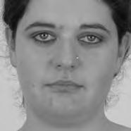
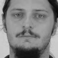
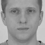
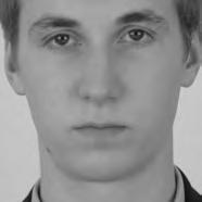
32 PUT Face Facetracer Figure 5.1: These two images are examples of faces from the two datasets. The left image is from PUT and there are 30 landmarks present. The right image is from Facetracer with 10 landmarks present. harder for even humans to distinguish between the people. However, since the images were taken under a controlled setting, we can see that there is better alignment among the faces, which is helpful for creating our face subspace. In addition, the high resolution helps with clarity and capturing fine details Facetracer The Facetracer[25] dataset is a highly diverse set of 15,000 face images. The image quality is not as good as PUT, but there are many more individuals to train from. Each face in Facetracer has 6 landmark points provided with the dataset, and we estimate 4 more landmark points. We estimate the nose by finding the center point among the labeled eyes and mouth. Then, we add three more points, the center of the mouth and the two nostrils sides. We estimate the nostrils sides by assuming they are not too far from the nose and manually analyze our guessed distances. The center of the mouth is the midpoint between the two mouth corner landmarks. Again, we take only the frontal faces in the dataset, in order to be consistent with SCiFI. We take a more unsupervised approach in pruning Facetracer because of its sheer size. Since faces that are frontal are going to be fairly symmetric, we try to find faces with unsymmetrical landmarks by determining the distances among different landmarks. We also remove all images with small children and images with resolutions less than , because they can have ambiguous features. There are 307 female and 394 male images or 701 images in the entire dataset, and there are roughly 600 unique individuals in total. Figure 5.3 provides examples of faces from the Facetracer dataset. We can see that 30

33 Figure 5.2: Here we have 30 examples of images in the PUT dataset. It is apparent that PUT is not very diverse. There are very few women subjects and most of the other individuals are Caucasian males. 31

34 Figure 5.3: Here we have 30 examples of images in the Facetracer dataset. It is apparent that Facetracer is a diverse dataset, for it is comprised of images from various races and genders. 32

35 there is certainly a diverse set of individuals in the dataset, which helps to provide a rich vocabulary. However, as opposed to PUT, we can see that the faces are not taken under the same control settings (e.g lighting conditions, face orientation/pose). This makes alignment and normalization among images more difficult. 5.2 Methodology In each experiment, we take care to ensure that a novel test face belongs to an individual that is not present in the data used for the public collection Y, which builds both the vocabularies and face subspace. To do this, but still allow maximal use of the data, we perform multiple folds for each experiment, each time removing a test individual and rebuilding the vocabularies and subspace with images only from the remaining individuals. This constraint is important to avoid giving our reconstruction algorithm any unfair advantage that it would not have in a real application. Our approach takes the binary facial vector as input, which in practice would be the data extracted during a SCiFI attack. Thus, for all experiments, we generate the facial vectors to perform our reconstruction. This is fairly simple given the labeled landmark points of every face in both datasets. For each landmark point of a given face image, we simply crop out a patch to be the same size as the the ones extracted to form the appearance vocabularies. In addition, we also compute the distance from each landmark and the nose (center) landmark. Now, we find the n closest appearance words and the z closest spatial words as defined by the SCiFI facial representation (Section 3.2). As described in Section 4.1.1, we can either use HOG descriptor or regular pixel intensities to determine this ranking. Therefore, we test both methods in our experiments. To be consistent, if we cluster with HOG, we also rank the vocabulary words with HOG. We do the same with the raw pixel intensities. 5.3 Implementation Details In this section, we will provide implementation details, such as the number of landmarks and the vocabulary size of our facial reconstruction approach, for both datasets. PUT We crop out only the face regions from each image (i.e., removing torsos), and rescale them all to a canonical size ( ). Although PUT provides us with 30 landmark points, we only use 24 of these points. This is because 6 of these points lie on the edge of the face and have a lot more noise (including hair and earrings). Consequently, we have the 24 landmarks as a facial part, so that gives us p = 24. For each landmark/part, we extract a patch that is 10% of the canonical face scale. We convert each patch into a HOG descriptor and use k-means clustering on the descriptors and distances to quantize the respective spaces. Following [1], we let each appearance vocabulary have N = 20 words, each distance vocabulary have Q = 10 words, and each encoding use n = 4 words for appearance and z = 2 for distances. This means that each of the 24 parts on a face is represented by four appearance patches and two quantized distances. Figure 5.4(b) shows an example of PUT appearance vocabularies used in our approach. 33

36 (a) Facetracer Male appearance vocabulary where p = 10 and N = 40. (b) PUT Faces appearance vocabulary where p = 24 and N = 20. Figure 5.4: Example appearance vocabularies for each dataset. (a) is formed from the Facetracer dataset and (b) is formed from the PUT dataset. Each row is a different part and each column is a prototypical word in the vocabulary. We can see a fairly clear distinction between the diversity of the prototypical words for the two datasets, where Facetracer is more diverse. 34

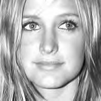
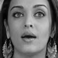
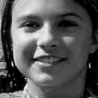
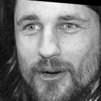
37 When computing the face subspace, we further reduce the resolution of the faces by 25%, to minimize computational costs. We use K = 194 eigenfaces based on analyzing the eigenvalues to determine how many eigenvectors would represent 95% of the variance in the data. Finally, we run the PCA algorithm with ɛ =.0001 and a maximum number of 2000 iterations. (We did try other values, and saw similar results for much fewer maximum iterations.) Each reconstruction is computed very quickly; on average, it takes about five to ten seconds and converges within 1500 iterations. Facetracer We also crop these images and rescale them to a canonical size of ( ). The images have a much lower resolution than PUT, but they are more diverse. As such, let each appearance vocabulary have N = 40 words, each distance vocabulary have Q = 10 words, and each encoding use n = 4 words for appearance and z = 2 for distances. Since Facetracer is much more diverse, we find that a larger N helps with matching characteristics of the original face. Figure 5.4(a) shows examples of Facetracer appearance vocabularies used in our approach. When computing the face subspace, we are not required to reduce the resolution. K = 695 for Facetracer based on analyzing the eigenvalues to determine how many eigenvectors would represent 95% of the variance in the data. Before we run the PCA reconstruction algorithm, we also apply a sharpening filter to the patch face. Sharpening the patch face helps with the Facetracer data because the resolution is so low. If we do not, some of the features may be lost. Finally, we run the PCA algorithm with ɛ =.001 and a maximum number of 2000 iterations. Each reconstruction is computed very quickly; on average, it takes about three to seven seconds and converges within 1200 iterations. For either dataset, when we do the patch face reconstruction as described in Section 4.2.1, there are patches that overlap their neighbors. Rather than selecting a priority on which patch should be placed over another, we simply average the overlapping pixel values together. This is not ideal since some information is lost, but if the patch sizes are small enough so that there is little overlap, the effect is very minimal. 5.4 Experimental Results In this section we describe each test and analyze the results Qualitative Results Figures 5.5, 5.6, and 5.7 display example reconstructions from the Facetracer and PUT datasets. Figure 5.6 shows our reconstructions using only male or female faces to construct the appearance and spatial vocabularies and the face subspace. We want to evaluate the qualities of our reconstructions when we separate gender features. Across the two datasets, we see that the reconstructed faces do form fairly representative sketches of the true underlying faces. We emphasize that the reconstructed image is computed directly from the encoding recovered with our cryptographic attack; our approach has no access to the original face images shown on the far left of each triplet. The fact that the full face reconstructions differ from instance to instance in the regions outside of the patch locations demonstrates that we 35

38 are able to exploit the structure in the face subspace effectively; that is, the surrounding content depends on the appearance of the retrieved quantized patches. In examining the reconstructions, we notice that the quality between Facetracer reconstructions using both males and females is slightly worse than the Facetracer reconstructions with specific gender. This is to be expected, for reconstructing in a gender specific vocabulary and face space guarantees that the specific gender s characteristics are going to be synthesized. There is no clear distinction on what gender has better reconstructions in Facetracer. On the contrary, the reconstruction of females in PUT are poorer than those of males. This is well-explained by the gender imbalance in the PUT dataset, where only 8 of the 83 individuals are female. This biases the face subspace to account more for the masculine variations, and as a consequence, the reconstructed faces for a female s facial encoding tend to look more masculine. Nevertheless, we can see that the general structure of the internal features is reasonably preserved. Of course, in a real application one could easily ensure that the public set Y is more balanced by gender. The blurry nature of the full face reconstructions are also to be expected, since the subspace technique is sensitive to the pixel-wise alignment of all images. One could ameliorate this effect with more elaborate subspace methods that account for both shape and appearance (e.g., active appearance models [7]). In addition, a larger public dataset and finer quantization of the vocabularies (higher Q and N) will yield crisper images. However, for our application, even a blurry sketch is convincing, since its purpose is primarily to suggest the identity of the recovered individual, and not to paint a perfect picture. Comparing the face reconstructions between the Facetracer and PUT datasets, there is definitely a certain generic look in most of the PUT reconstructions. This can be attributed to the smaller dataset with fewer unique individuals. However, the higher resolution and more landmark points of the PUT images also affect PUT s reconstruction. Compared to the Facetracer reconstructions, the reconstructions tend to be more sharper and well defined. With more landmark points, the PCA technique has more information in its iterative refinement steps. There is less information that needs to be hallucinated compared to Facetracer. Although the Facetracer reconstructions are not as sharp, they tend to capture more of the facial expressions and facial features of the original face. With more data, there is a higher chance that another person s face shares similar qualities with the target face during reconstruction. We expect more refined reconstructions with higher quality datasets. However, our results are rather quite impressive with these two datasets. Given the course binary face encoding, we are able to reconstruct human faces of police sketch quality. Therefore, our qualitative results show that our reconstruction approach is a compelling visual extension of the SCiFI attack Quantifying Reconstruction Error Next we quantitatively evaluate the quality of the reconstructions of each dataset. By definition, our patch face reconstructions are as correct as possible, having only the error induced by the quantization of the vocabularies. Thus, we focus on the relative quality of our full face reconstructions compared to three baselines. 36

39 Figure 5.5: This figure shows 24 qualitative reconstruction examples from the Facetracer dataset, utilizing both males and females to build the vocabulary and subspaces. Each triplet is comprised of the true face, patch face, and reconstructed face. It is important to note that our reconstruction algorithm does not have access to the true face (far left image). It is apparent that Facetracer is a diverse dataset, for it is comprised of images from various races and genders. We can see distinct features in many of the results. 37

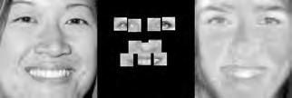
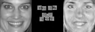
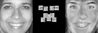
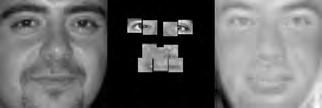
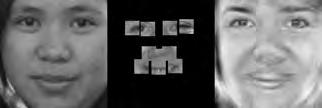
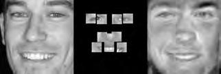
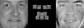
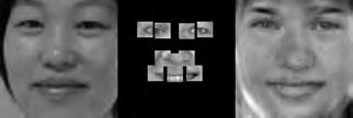
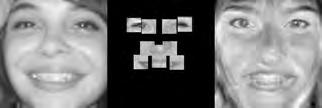
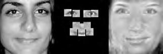
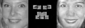
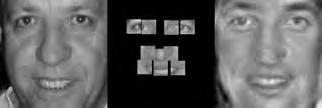
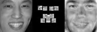
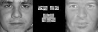
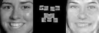
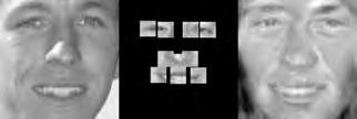
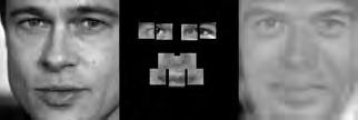
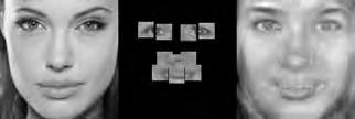
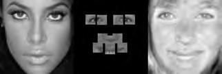
40 Figure 5.6: This figure shows 24 qualitative reconstruction examples from the Facetracer dataset, where males are reconstructed from a purely male vocabulary and male subspace; similarly for the female reconstructions. Each triplet is comprised of the true face, patch face, and reconstructed face. It is apparent that Facetracer is a diverse dataset, for it is comprised of images from various races and genders. We can see distinct features in many of the results. 38

41 Figure 5.7: This figures shows 24 qualitative reconstruction examples from the PUT dataset. Each triplet is comprised of the true face, patch face, and reconstructed face. It is important to note that our reconstruction algorithm does not have access to the true face (far left image). Most of PUT s subjects share similar characteristics and the majority are Caucasian males. Thus, the reconstructed faces are fairly similar as well. 39

42 Figure 5.8: This figure shows how the quantifying reconstruction error test is designed. The goal of this test is to show that the error between the truth face and the reconstructed face is less than the error of the other three baselines. Therefore, the distance between the truth face and the baselines and reconstruction face are computed to measure the error. Then by subtracting the reconstructed face s error from the error of the baselines, we can compute the positive or negative agreement gain. The first baseline is a randomly reconstructed face. We implement a method that randomly selects the appearance vocabulary words and spatial words, but otherwise follows our full face reconstruction approach to form a random face. The second baseline compares our reconstructed face to its original patch face. The final baseline is the mean face overlaid with our patch face. The mean face is obtained during the construction of our face subspace. This face has very generic human face features. Figure 5.8 illustrates this experiment s setup. For our method and all baselines, the goal is to be as close as possible to the true original face image. To compare our reconstruction against these baselines, we consider the distance in the HOG [21] feature space between the reconstructed faces and the original faces. In particular, we use a HOG descriptor with the following parameters: 16 histogram bins with a 4 4 window size. We compute the distance between our reconstructed face and the true face; for each baseline we also compute its distance from the true face. We plot the distribution of the agreement of the full face reconstruction method versus each of the baselines. Figure 5.9 shows the results. Our four plots are organized as follows: each row is a differ- 40

43 FT HOG FT 1 1 Improvement Over Baselines Improvement Over Baselines Random Face Patch Face Mean Face + Patches Baselines 1 Random Face Patch Face Mean Face + Patches Baselines PUT HOG PUT 2 2 Improvement Over Baselines Improvement Over Baselines Random Face Patch Face Mean Face + Patches Baselines Random Face Patch Face Mean Face + Patches Baselines Figure 5.9: This figure shows the results of quantifying the reconstruction qualities of our two datasets. Each row is a different dataset and each column uses a different method of clustering and facial part matching. The boxplots in general show an increase in correlation with the ground truth achieved by our full face reconstruction relative to the randomized baseline (left), the initial patch face reconstruction (middle), and the mean face with patches overlaid (right). Red center bars denote median values; boxes above and below represent upper and lower quartile values. Values above zero indicate improvement; higher is better. Our full face sketch produces a visualization most closely resembling the true underlying face in each of the datasets. 41

44 ent dataset and each column uses a different method of clustering and facial part matching (left column uses HOG and the right column uses raw pixel intensities). In each boxplot, we display the agreement of our method versus the randomized baseline (left), the initial patch face reconstruction (middle), or the mean face with patches overlay (right). Each boxplot shows the distribution of agreement across all test cases for each dataset, and any positive value indicates that our full face reconstruction more closely resembles the true face. Compared to the patch face, our approach clearly synthesizes a face closer to the true face. This is because the patch face has a significant amount (60%-80%) of missing facial information. Compared with the mean face overlaid with the patch faces, our reconstructions are still much closer to the true face. However, since the mean face does provide a generic face we can that this baseline is stronger than the patch face by itself. Now compared to the random face, the error margin is closer between them than the other two baselines. However, our reconstructions are still doing better than a random face. These three consistent results show that our reconstructions are much closer to the original face than purely what is given to us by the SCiFI facial vector alone Machine Face Recognition Experiment The goal of this experiment is to test how well a computer can match and rank our reconstructed face with other real faces in the database. This experiment is complemented by a human experiment in the following subsection. We input into the computer a reconstructed face and a database, T, of truth/original faces. The reconstructed face is synthesized through our full facial reconstruction approach. The original face, unavailable to our reconstruction algorithm, is also in T. Now, we have the machine rank each face in the set T from 1 to T (with no ties), where the lower ranks indicate higher correlation. In order to perform the ranking task, we have the computer compute a distance from the reconstructed face and each of the true faces. However, there is an issue that arises from doing a direct comparison of a true face and its reconstructed face. The two images are in two different image spaces. Therefore, we use Information Theoretic Metric Learning (ITML) to learn a Mahalanobis matrix, A, and use the learned Mahalanobis distance to rank our images [27]. The Mahalanobis distance, M d, of two images x = [x 1, x 2,..., x n ] t and x = [x 1, x 2,..., x n] t where n is the size of the image is defined as: M d (x, x ) = (x x ) t A(x x ) Figure 5.10 provides an illustration motivating learning a Mahalanobis distance. The ITML algorithm takes in three inputs: a set of instances X, their labels Y, and a series of similarity and dissimilarity constraints Z. Each true face and its reconstructed face are instances in X and they are given the same label in Y. We learn the Mahalanobis matrix using a separate training set, and then we test the learned distances on a held out test set. For testing Facetracer, we learn a Mahalanobis matrix from 600 Facetracer instances that were not used in our earlier experiments. These faces include images that are labeled properly, but were excluded due to our previous strict requirements of alignment and frontal pose. For PUT, we use a 4-fold cross-validation since our dataset is very limited. We manually construct constraints that show that each true face is similar with its 42

45 Figure 5.10: This figure shows how we learn the Mahalanobis distance. Initially, the truth face and reconstructed faces are in two different image spaces, such that the corresponding pairs of truth and reconstruction faces are not close in the Euclidean space (matrix A 0 ). However, using ITML, similarity constraints can be set such that corresponding truth and reconstructed faces are close and dissimilarity constraints can be set to push away other images. The right box shows the learned Mahalanobis distance (A) that captures these constraints. reconstructed face given that their Mahalanobis distance is less than an upper bound u. Likewise, every reconstructed face is dissimilar to other reconstructed faces given that their Mahalanobis distance is greater than a lower bound l. We found that with and without dissimilar constraints, our results were comparable. The values of u and l are the 95th and 5th percentile distances from all the truth faces and their reconstruction pairs. The ITML algorithm produces a metric parametrization that preserves these constraints and therefore can better compare novel instances of reconstructed faces to their real image counter parts. Figure 5.11 shows the plots of the ranks for the ITML learned distance compared to two baselines. Each point indicates the percentage of images ranked within the first R ranks. For example, if R = 10, then our graph indicates the percentage of the corresponding true faces ranked either 1, 2,..., or 10 for every reconstructed face. The first baseline is Euclidean distance. We can see that the learned Mahalanobis distance ranks the reconstructed face and its corresponding true face closer than Euclidean distance. This indicates that we can learn a better measurement between our reconstructed faces and the original images. Our second baseline is a random ranking of each reconstruction compared to the database of true faces. Here, we can see that our learned distance and Euclidean distance is better than randomly selecting a rank for the corresponding true face. 43

46 1 Facetracer 1 PUT Recognition Rate Recognition Rate Learned Mahalanobis Distance Euclidean Distance Expected Ranking (Random) Learned Mahalanobis Distance Euclidean Distance Expected Ranking (Random) Ranks Ranks Figure 5.11: This figure shows the ranking results from the Machine Face Recognition test. The learned Mahalanobis distance and Euclidean distance perform better than random chance. Each plot shows the rank-r recognition rate that the reconstructed face is ranked to its true face within in the top R rank for each face Human Experiment The human experiment tests show how easily recognizable our reconstructions are. We want to see how well an outside observer would recognize the synthetic faces out of context. Therefore, we have 30 individuals take our human test. The participants are not involved with this project and are a mix of students and non-students. We use the Facetracer with a female vocabulary and face subspace to perform this test. For clustering and constructing a fragmented patch face, we use pixel intensities as opposed to HOG [21]. We choose not to use HOG because the qualitative results for this dataset seem to be better with the pixel intensities. For this test, we have 30 test pages, and on each page we provide the subject with a reconstructed face and four normal faces. We ask the user to rank the four original/truth faces from 1 to 4 (1 being the closest) according to how close they thought the face was to the reconstructed face. Figure 5.12 shows a screenshot from the test. This test is similar to a police line up. We record their answers for rank number 1 and rank number 2. It is important to note that each real face must be ranked a different value. The results from the test are in Figure We show the subject s accuracy based on only their first guess (left), or based on either of the first two guesses (right). The results are very promising because in cases of correctly identifying the original face in one and two attempts, random chance is 25% and 50%, respectively. The subjects did much better than random chance, for they averaged 41% and 62% accuracy, respectively. We also include the accuracy of a machine performing the identical task as the human subjects. We can see the machine correctly identifies the original face in one and two attempts with 50% and 73% accuracy. The machine uses a learned Mahalanobis distance such as in Section Although the machine is not perfect, it still does far better than chance; thus, strengthening the effectiveness of our reconstructions. Our experiment shows that this test is not trivial. We crop out the hair, neck, and even 44

47 Figure 5.12: This is the SCiFI Human Reconstruction human subject experiment interface. The top row of images is the reconstructed face (repeated 4 times). The task for the tester is to rank from 1 to 4 (1 being the best match) to how close each face in the second row is to the first row. ears of the individuals, which make this task very difficult. Subjects are not given much external information to aid them in this task, and we do not have any images of men in the multiple choice options either. In addition, when interpreting these results, one must recall that under the SCiFI recognition system there is a lossy representation that will make certain faces indistinguishable. Figure 5.14 shows a table of questions and the number of correct answers associated with the question. The significance of this table is the distribution of correct answers for each question. The distribution is not uniform. Questions 1, 4, and 16 are almost unanimously correctly answered, while questions 13, 17, 25 are missed most frequently. This shows us that there are clearly good and poor reconstructions. A uniform distribution would imply our reconstructions are all ambiguous and it was pure chance that we saw these results. Figure 5.15 shows the top and bottom most correct and most missed pairs. The left column s images share much more resemblance then the right column s images. This shows the practical importance of our facial reconstruction in providing recognizable faces that are not solely provided by extracting a facial vector. As shown by our qualitative results, our reconstruction does synthesize human faces from a fragmented patch face assembled from the facial bit vector. This is very impressive, since we are given a very course representation of a face that is missing a lot of information. Our 45

48 Figure 5.13: This figure shows the accuracy with which the 30 human subjects could predict the correct face match for 30 test cases given our algorithm s automatically reconstructed image. We report their accuracy when looking at their first guess only (left boxplot) or either of their first two guesses (right boxplot). Red center bars denote median values, and boxes above and below the red bars represent upper and lower quartile values. As one can see, humans perform much better than random chance (green dash-line). We also included the accuracy of a machine (purple dash-dot-line) performing the same test as the human subjects. quantitative results show that our reconstructions are the closest facial synthesis to their corresponding true faces, and that the reconstructions are machine and human recognizable. In the next chapter, we will reflect upon our approach. 46

49 Question One Guess Two Guesses Question One Guess Two Guesses Figure 5.14: This table shows, for each question, how many participants got correctly on their first guess or by their second guess (includes their first guess). It is important to notice there are distinct test pages that all users do well on and others that all users do bad on. This shows that there is agreement on what are good and bad reconstructed faces. Highest Percentage Correct Lowest Percentage Correct Figure 5.15: These images show the top correct and missed reconstruction tests. The left column is the top three questions correctly answered, and the right column is the top three questions missed. 47