Computer Graphics. Graphic pipeline OpenGL, DirectX etc

Transcription

1 OpenGL, DirectX etc 1

2 Approach that is complementary to ray-tracing Lots of different implementations Software implementation e.g. Pixar Renderman Do a 2 hours movie in 1 year imposes leaves less than 3 minutes of CPU time per image (but it is easily run un parallel) Hardware implementations, e.g. PC graphic cards Goal here : speed but also some realistic rendering (very flexible) Almost realtime : rendering of many millions of triangles per second In what follows, we will restrict ourselves to an abstraction of an hardware implementation 2

3 Goal here : operations are easily parallelized or vectorized Groups of dedicated GPUs that are able to execute dozens to thousands ot operations in parallel explains why GPUs are so powerful ( many times that of generic CPUs à 1/5 of the clock speed) Dedicated high-bandwith memory 3

4 Bus performance (dates back to 2010 but ideas are same today) Nvidia 4

5 GPU specific architecture Nvidia 5

6 Pipeline Application Command flow vertex processing We are here «Langage» standards OpenGL, DirectX etc... 3D Transformations shading Transformed geometry Raster conversion Fragments ( ~ pixels + interpolated data) Operations on fragments (fragment processing) Conversion of primitives into fragments Compositing, mixing, (shading) framebuffer Display What the user sees 6

7 Primitives Points (in space) Line segments Triangles Polylines Triangle fans / strips That s all! Curves? Transformed into polylines Polygones? Decomposed into triangles Curved surfaces? Approximated with triangles The current «trend» is the restrict to a minimal number of primitives Simple, uniform, repetitive good for vectorial processing 7

8 Command flow : depends on the implementation e.g. OpenGL 1, DirectX, others Always somewhat similar See OpenGL labs OpenGL advantages : Multiplatform, simple, high performance, still evolving, and not attached to a specific architecture or company. It became a standard and is supported everywhere, even on smartphones 8

9 Pipeline Application Command flow vertex processing We are here «Langage» standards OpenGL, DirectX etc... 3D Transformations shading Transformed geometry Raster conversion Fragments ( ~ pixels + interpolated data) Operations on fragments (fragment processing) Conversion of primitives into fragments Compositing, mixing, (shading) framebuffer Display What the user sees 9

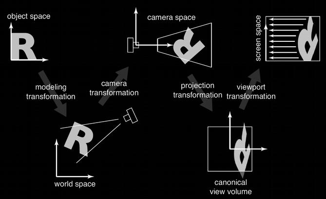
10 Pipeline of geometrical transformations 10

11 11

12 Clipping Rasterization expects that primitives are visible on the screen This is done in the 3D canonical space, after the application of the perspective projection (see course 2 ), but before the perspective division. All that is outside the volume limited by : w x w w y w w z w is discarded Cut by 6 planes 12

13 Clipping Basic operation : cut a triangle into 3 by a plane 4 cases : All vertices inside tr kept All verticels exterior triangle discarded 1 vertex in; 2 out 1 triangle remains 2 vertices in; 1 out 2 triangles remain 13

14 Hidden face removal We have seen how to geometrically transform the primitives to the screen The perspective projection gives a strong hint on depth Hidden face removal is another strong hint Allows to draw exclusively what is seen (goal : performance) 14

15 Hidden face removal Backface culling For closed and opaque shapes, one does not see the inside! 15

16 Hidden face removal Backface culling No need to draw the backward-facing faces v n n v 16

17 Hidden face removal Backface culling No need to draw the backward-facing faces v n v n 0 n v 17

18 Hidden face removal Backface culling Dépends ont the convention used to compute the normal to the shape Usually, exterior pointing vector Computation is easy if triangles are carefully oriented! s3 s1 s 2 s1 s 3 n= s1 s 2 s1 s 3 s1 s2 18

19 Hidden face removal How to care for this case? Painter s algorithm Binary space partitionning Z-buffer 19

20 Pipeline Application Command flow vertex processing We are here «Langage» standards OpenGL, DirectX etc... 3D Transformations shading Transformed geometry Raster conversion Fragments ( ~ pixels + interpolated data) Operations on fragments (fragment processing) Conversion of primitives into fragments Compositing, mixing, (shading) framebuffer Display What the user sees 20

21 Raster conversion First stage : enumerate pixels that are covered by a «continuous» primitive Second stage : Interpolate values that are known on the vertices of the primitive Example : the colour known at the vertices of a triangle may be distributed on each pixel covered by the triangle Other variables may also be interpolated. Normal vectors for instance... 21

22 Raster conversion Transformation of continuous primitives into discrete pixels Example : drawing of a line Difficulty : aliasing 22

23 Naïve algorithm Line = unit width rectangle One specifies beginning and end vertices Case here : black inside and white outside 23

24 Naïve algorithm Line = unit width rectangle One specifies beginning and end vertices Case here : black inside and white outside 24

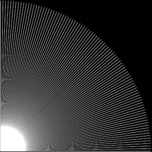
25 Point sampling One approximates the rectangle by drawing every pixel whose center is inside the rectangle 25

26 Point sampling One approximates the rectangle by drawing every pixel whose center is inside the rectangle Problem : sometimes pixels with more that one adjacency are turned on 26

27 27

28 Bresenham algorithm (midpoint alg.) We will define the thickness with respect to the y axis... 28

29 Bresenham algorithm (midpoint alg.) We will define the thickness with respect to the y axis... One turns on only one pixel per column 45 slanted lines will appear thinner. 29

30 Bresenham algorithm (midpoint alg.) We will define the thickness with respect to the y axis... One turns on only one pixel per column 45 slanted lines will appear thinner. 30

31 31

32 Bresenham algorithm (midpoint alg.) Equation : Evaluated for everu column y=mx b One turns on only one pixel per column y=0.49x x 0 x 1 0 m 1 6 for x = ceil(x0) to floor(x1) y=b+m*x plot(x,round(y))

33 Optimization Multiply and rounding are rather slow operations (at least on primitive CPUs) y=mx b mx b y=0 For each pixel, the only options are E and NE One computes the error : d > 0.5 decides E or NE d =m x 1 b y 7 6 NE 5 4 x, y 3 E

34 Optimization d =m x 1 b y One must only update integer steps along x and y Exclusive use of the addition (no mult or divide) d > 0.5 decides E or NE d =d 1 d =d m

35 Optimization x=ceil(x0) y=round(m*x+b) d=m*(x+1)+b-y While (x<floor(x1)) { If d>0.5 { y=y+1 d=d-1 } x=x+1 d=d+m plot(x,y) } // round to ceil // round to nearest // round to floor

36 Generally, endpoints are given G x, y 0 dy y= x +b dx x0 y0 x1 y1 G x, y =0 G x, y 0 dx= x 1 x 0 dy= y 1 y 0 Implicit form : G x, y =dy x dx y dx b F x, y =2 dy x 2 dx y 2 dx b 36

37 What is the value of F at M? d i = F x i 1, y i 1/2 =2 dy x i 1 2 dx y i 1/2 2 dx b d i 0 : M is under the line go to NE d i 0 : M is above go to E NE? M xi, yi Q E? 37

38 First point: what is the value of d 0? d 0=F x 0 1, y 0 1/2 =2 dy x dx y 0 1/ 2 2 dx b =2 dy x 0 2 dx y 0 2 dx b 2 dy dx =F x 0, y 0 2 dy dx As x 0, y 0 belongs to the line : F x 0, y 0 =0 d 0=2 dy dx 38

39 Recursion : what is the value of d i 1? If d i 0 then go to E : x i 1, y i 1 = x i 1, y i d i 1= F x 2, y 1/ 2 =d i 2 dy Otherwise go to NE : x i 1, y i 1 = x i 1, y i 1 d i 1= F x 2, y 3/2 =d i 2 dy 2 dx 39

40 Algorithm is valid only for one octant Bresenham( x1, y1, x2, y2 ) { dx = x2 x1 dy = y2 y1 d = 2*dy dx plot( x1, y1 ) while (x1 < x2 ) { if (d <= 0) // EAST d = d + 2*dy else // NORTH-EAST { d = d + 2*(dy-dx) y1 = y1 + 1 } x1 = x1 + 1 plot( x1, y1 ) } } 40

41 What to do if the line is not in the right octant? Exchange x and y Exchange start and end points Replace y by -y 41

42 Same type of algorithm do exist for other geometric shapes : e.g. circles (see litterature What about aliasing? Algorithm derived from Bresenham that avoid aliasing do exist, see algorithm of Xiaolin Wu Oversampling sampling on a finer grid then averaging on bigger pixels is also an option. Bresenham, Jack E. "Algorithm for computer control of a digital plotter", IBM Systems Journal, Vol. 4, No.1, pp , 1965 Wu, Xiaolin. "An efficient antialiasing technique". 25 (4): ,

43 43

44 Interpolation Some variable is known at the vertices of the triangle (color, normal vector, etc...) One wish to get a representative value of the same variable along the line for every pixel that is turned on. A progressive variation would be fine, thus a linear interpolation is the right tool here : f x = 1 f 0 f 1 1D : = x x 0 / x 1 x 0 2D,3D : a is simply the distance ratio to the endpoints. 44

45 Interpolation The pixels are not exactly on the line One defines a projection on the line It is linear One may use results obtained before to construct an interpolation P1 = v x / L P0 v = v y / L =v Q P 0 / L L=v P 1 P 0 45

46 Interpolation The pixels are not exactly on the line One defines a projection on the line It is linear One may use results obtained before to construct an interpolation P1 = v x / L P0 v = v y / L =v Q P 0 / L L=v P 1 P 0 46

47 Alternative meaning d and a are updated from pixel to the next pixel d tells us at which distance we are to the line a tells the position along the line d and a are coordinates in the natural frame of the line 47

48 Alternative meaning The loop means the pixels that we visit Interpolation of d and a at each pixel A fragment is emmitted if the pixel s center is in the band Interpolation becomes the main operator P1 P0 v u 48

49 Alternative meaning x=ceil(x0) y=round(m*x+b) d=m*(x+1)+b-y etc... while (x<floor(x1)) { if (d>0.5) { y=y+1 d=d-1 etc... } else { x=x+1 d=d+m etc... } If (-0.5 < d <= 0.5) plot(x,y, ) } P1 P0 v u 49

50 Triangle raster conversion Very common case With a good antialiasing, may be the only case! Some systems represent lines with two very thin triangles Triangle represented with 3 vertices The algorithm has the same philosophy as for lines : One walks from pixel to pixel Linear operators are evaluated for each step Those operators allow us to know if a pixel is inside or outside 50

51 Triangle raster conversion Input : Three 2D points x 0, y 0 ; x1, y 1 ; x 2, y 2 Variables to interpolate, at each vertex q 00,, q 0 n ; q10,, q1 n ; q 20,, q2 n Output : a list of fragments, with : Integer coordinates of pixels x, y Interpolated variables q 0,, qn 51

52 Triangle raster conversion Incremental evaluation of linear functions on a grid of pixels Functions are defined by the value at the vertices Use of additional functions to determine the set of fragments to return back Vertex Fragment x 0, y 0 q 00,, q 0 n x 2, y 2 q 20,, q 2 n (x, y) q 0,, q n x 1, y 1 q10,, q1 n 52

53 Incremental linear interpolation A linear affine function in the plane : q x, y =c x x c y y c k Evaluation on a grid is efficient : q x 1, y =c x x 1 c y y c k =q x, y c x q x, y 1 =c x x c y y 1 c k =q x, y c y +cy +cy... +cx+cx +cx... 53

54 Interpolation of variables known at vertices Determine c x, c y, c k defining the unique linear function that gives back the value at the vertices 3 parameters, 3 equations : c x x 0 c y y 0 c k =q 0 c x x 1 c y y 1 c k =q1 c x x 2 c y y 2 c k =q 2 x0 x1 x2 y0 1 cx q0 y1 1 c y = q1 y2 1 ck q2 Singular system if points are collinear 54

55 Interpolation of variables known at vertices Translation of the origin to x 0, y 0 q x, y =c x x x 0 c y y y 0 q 0 q x 1, y 1 =c x x 1 x 0 c y y 1 y 0 q 0 =q 1 q x 2, y 2 =c x x 2 x 0 c y y 2 y 0 q 0=q 2 2X2 linear system x 1 x 0 y 1 y 0 c x q 1 q 0 = x 2 x 0 y 2 y 0 c y q 2 q 0 Solution using Cramer s rule c x = q 1 y 2 q 2 y 1 / x 1 y 2 x 2 y 1 c y= q 2 x 1 q1 x 2 / x 1 y 2 x 2 y 1 55

56 What are the fragments to consider? Those for which the barycentric coordinates are positive Algebraically, on has c,, p= a b c =1 Inside iff 0 ; 0 ; 0 a b Pineda, Juan, " A parallel algorithm for polygon rasterization" 22 (4): 17-20,

57 Barycentric coordinates are interpolated variables Each barycentric c. yields 1 on a specific vertex and 0 on all others. They are an implicit representation of the sides of the triangle. 57

58 Pixel-per-pixel raster conversion (Pineda s algorithm 1998) One vists conservatively a superset of the pixels Use of interpolation of linear functions Use of barycentric coordinates to determine when to emit a fragment x 2, y 2 q 20,, q 2 n x 0, y 0 q 00,, q 0 n x 1, y 1 q10,, q1 n 58

59 Triangle raster conversion Beware of rounding and arbitrary decisions One has to visit every pixel at least once... (otherwise there may be a hole!) But not two times! (Those pixels would take an arbitrary colour that depend in which order things are drawn) Elegant solution : antialiasing... 59

60 Pipeline Application Command flow vertex processing We are here «Langage» standards OpenGL, DirectX etc... 3D Transformations shading Transformed geometry Raster conversion Fragments ( ~ pixels + interpolated data) Operations on fragments (fragment processing) Conversion of primitives into fragments Compositing, mixing, (shading) framebuffer Display What the user sees 60

61 Z-buffer (depth buffer) In many application, sorting with respect to depth is too costly The order changes with the viewpoint There exists the BSP tree Viewpoint independent but : Heavy datastructures (difficult to implement «in silico») Cutting of primitives Slow building Non-incremental (all data have to be known in advance) 61

62 Solution that is usually favoured : draw in any order and keep track of the closest drawn pixel Use an additional storage, that stores, for each pixel, the smallest depth to date When one ought to draw a new pixel, the actual depth is compared to the stored depth and if the latter is greater, then the pixel is drawn and the depth is updated. 62

63 Z-buffer This is an axemple of a «brute-force» approach, it works because memory is cheap and fast. Foley et al. 63

64 Z-buffer Evidently limited to bitmap images (not vectorial) Somewhat more difficult to implement with transparency (alpha channel) 64

65 Z-buffer and alpha channels One separates opaque objects and translucent ones 1) Opaque objects are drawn with an update of the z-buffer. 2) Then, use a BSP tree for partially transparent entities 3) Draw transparent entities using the BSP ordering, while takin the Z-buffer into account, but without updating it Thus, transparent faces behind opaque ones are not drawn (they are not visible) 65

66 Z-buffer : limited accuracy The supplementary channel is generally encoded as an integer, as are the color channels 0< z * < N 1 Cause : hardware implementation (simple and fast) It is possible to have distinct objects seen at the same depth if the value that is stored in the Z-buffer is the same The accuracy is spread between n (near plane) and f (far plane) These were used to define the observable volume, see course 2. 66

67 Z-buffer Plane n * Plane f z *= N 1 z =0 67

68 Z-buffer Let us choose an integer with b bits (8 or 16...) What is then the accuracy of the z-buffer? If the z that is stored is proportional to the actual distance (case of orthogonal projections): We have N=2b layers for a distance equal to f-n Therefore, the accuracy (independent to the distance!) is Δ z= ( f n) 2b : to maximize the accuracy, f-n must be kept small. If a perspective projection is used, the z stored in the z-buffer is proportional to the result obtained after the perspective division. Therfore, the size of the layers depends on depth By how much? 68

69 Z-buffer Plane n * z =0 Plane f z *= N 1 Orthographic proj. Perspective proj. 69

70 Z-buffer In the second course, we have computed zc after the perspective divide : 2 n r l 0 x, y, z,1 r l r l n 0 0 f n 2 f n t b = X,Y, z, z n f n f t b f n 1 t b n f f n 2 f n 2 f n z c= 0 0 n f f n z f n M proj _ persp _ OpenGL z c= f n 2fn f n z f n 70

71 Z-buffer The interval for zc is 2 ( -1 to 1) and one still have N layers. z c= f n 2fn f n z f n z c 2 z f n 2 = 2 z f n N What is the size of the layers? Need to solve for z (invert) The largest layer is for z=f : 2 z f n z= N fn z max = f f n Nn 71

72 Z-buffer Example: n = 1 m, f = 100 m, the z-buffer has 8 bits N=256, what is the actual size of the layers? 2 z f n Δ z = f ( f n) = =39 m (0.15 m with 16 bits) z= max Nn N fn n f n 1 99 z min = = = m N f With n=10 : f ( f n) Δ z max = = =3.5 m (0.013 m with 16 bits) Nn n f n z min = = =0.035 m 72 N f

73 Z-buffer For a good accuracy, it is best to increase n and decrease f. Never ever set n=0 cancels the z-buffer Generally, the number of bits b is fixed by the hardware (usually 16, 24 or 32 bits) The more the better but takes as much memory as the picture (usually 24 bits) 73

74 Interpolation in perspective projection projection plane eye Projections of the endpoints 74

75 Interpolation in perspective projection projection plane p2 eye p 1 p 2 2 p1 Projection of the middle of the line middle point of the projected line Linear interpolation in screen coordinates interpolqtion in eye space 75

76 Interpolation in perspective projection projection plane eye Projects in the middle... z1 z 1 z 2 /2 z2 Projection of the middle of the line middle point of the projected line Linear interpolation in screen coordinates interpolqtion in eye space 76

77 Interpolation in perspective projection Projection plane eye equidistant on z Projection of the middle of the line middle point of the projected line Linear interpolation in screen coordinates interpolqtion in eye space 77

78 Interpolation in perspective projection Projection plane eye This projects in the middle z c1 z c1 z c2 / 2 z c2 Projection of the middle of the line middle point of the projected line Linear interpolation in screen coordinates interpolqtion in eye space 78

79 Interpolation in perspective projection Projection plane eye equidistant on z c (screen depth) The depth variable that has to be interpolated (at the pixel level is zc (screen depth) obtained after perspective divide, and not z, the real coordinate 79

80 The perspective correction (use of zc instead of z ) aims to avoid problems for e.g. textures applied on slanted surfaces F0 wikipedia F1 F u = 1 u F 0 u F 1 F0 1 u u z c0 F u= 1 1 u u z c0 F1 z c1 1 z c1 80

81 Minimal pipeline «Vertex» stage (input : 3D positions / vertices and colors / triangle) Position transformation (object space eye space) Position transformation (eye space screen space) Transmission of the color (no interpolation = constant on the triangle) Raster conversion Pixel list Transmission of the color «Fragment» stage (output : color) Display pixels with right colors on the frambuffer 81

82 82

83 Minimal pipeline with z-buffer «Vertex» stage (input : 3D positions / vertices and colors / triangle) Position transformation (object space eye space) Position transformation (eye space screen space) Transmission of the color (no interpolation = constant on the triangle) Raster conversion Interpolation of zc (z in screen space) Transmission of the color «Fragment» stage (output : color, zc) Display pixels with right colors on the frambuffer and update z-buffer only if z c < current zc 83

84 84

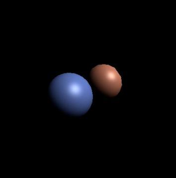
85 Flat shading Uses the «real» normal to the triangle Faceted appearance Most realistic view of the real geometry (as defined) Foley et al.85

86 Minimal pipeline with z-buffer and flat shading «Vertex» stage (input : 3D positions / vertices and colors / triangle + normal) Position transformation (object space eye space) Color computation (flat shading) with the normal (one color / tri) Position transformation (eye space screen space) Transmission of the color (no interpolation = constant on the triangle) Raster conversion Interpolation of zc (z in screen space) Transmission of the color «Fragment» stage (output : color, zc) Display pixels with right colors on the frambuffer and update z-buffer only if z c < current zc 86

87 Flat shading 87

88 Observer and illumination : close vs. far Phong illumination require some geometric info Light vector (depends on position) Obsever vector (depends on position) Normal to the surface (computed beforehand) Observer & light vectors are changing Must be computed & normalized for every facet light observer 88

89 Observer and illumination : close vs. far Case where observer and source are far away Almost parallel light rays Almost orthographic projection Light & observer vectors do not change much A frequent optimization is to consider they do not change even though it is generally false 89

90 Directional light (e.g. sun) Light vector is constant light [ x y z 0] observer In many cases, it increases dramatically the throughput of the pipeline by simplifying computations 90

91 Observer at the infinite Orthographic projection? Constant projection angle One may also do that for the perspective projection, only for shading computations The observer vector is considered constant (for instance, it is normal to the image plane) Yield strange results if a wide angle view is used Blinn-Phong shading: observer, light, and bisector vector all constant (see course 4) 91

92 Directional light & far observer light [ x y z 0] observer [ x o y o z o 0] Only the normal changes. Means the shading of every facet is the same if the orientation is the same. 92

93 Gouraud interpolation One wants a smooth shading eventhough the geometry is faceted Remember mapping : sensitivity to the normals much greater than the sensitivity to positions Idea : colour is computed at the facet s vertices Then, an interpolation is performed to get the color everywhere, at same time than the raster conversion. 93

94 Gouraud interpolation Foley et al.94

95 Pipeline with z-buffer and Gouraud interpolation «Vertex» stage (input : 3D positions / vertices and color per triangle + normal per vertex) Position transformation (object space eye space) Color computation made per vertex Position transformation (eye space screen space) Raster conversion Interpolation of zc (z in screen space), rgb color «Fragment» stage (output : color, zc) Display pixels with right colors on the frambuffer and update z-buffer only if z c < current zc 95

96 Pipeline with z-buffer and Gouraud interpolation 96

97 Gouraud interpolation Normals at vertices Mathematically undefined If the tessellation (triangulation) is obtained from a smooth surface (sphere, B-Spline, etc..), one may take the exact normal on that surface at the vertex If not, just do as if by averaging neigboring triangle normals N1 Ni N5 Ns N4 N3 N s= N2 i Ni i 97

98 Gouraud interpolation May be applied to any shading model Diffuse Blinn-Phong Etc... However, for specular shading, it does not work well There are strong variations of the shading with respect to the position, even on a single triangle. A linear interpolation is just too basic to reproduce these variations. 98

99 Blinn shading and with Gouraud interpolation 99 Foley et al.

100 Phong interpolation Why not interpolate normals and compute shading at the pixel (fragment) level? As easy as interpolating colors The shading will be computed are every pixel, from information that have been interpolated (colors, normals, etc... In the, it means that we move the shading computation from the «Vertex» stage to the «fragment» stage. 100

101 Pipeline Application Command flow vertex processing We are here «Langage» standards OpenGL, DirectX etc... 3D Transformations shading Transformed geometry Raster conversion Fragments ( ~ pixels + interpolated data) Operations on fragments (fragment processing) Conversion of primitives into fragments Compositing, mixing, (shading) framebuffer Display What the user sees 101

102 Pipeline with z-buffer and Phong interpolation «Vertex» stage (input : 3D positions / vertices, triangle, + normal/color per vertex) Position transformation (object space eye space) Position transformation (eye space screen space) Raster conversion Interpolation of zc (z in screen space), rgb color, xyz normal «Fragment» stage (output : color, zc) Shading computation using interpolated data (including normal) Display pixels with right colors on the frambuffer and update z-buffer only if z c < current zc 102

103 Phong interpolation 103

104 OpenGL Some shading models are part of the standard (typically : Phong, Lambert, Gouraud, Blinn-Phong ), Nothing has to be done. For specific shading computations, there is an API that allows defining exactly what has to be done at each stage : Either at the «vertex shader» stage, vertex per vertex Or, at the «fragment shader» stage, pixel per pixel Recent graphic cards (and the software driver embedded in the operating system) allow to litterally program in pseudo C-language either the «vertex shader» or the «fragment shader» (see e.g. Nvidia CUDA, OpenCL) 104

105 Programmable! Not very versatile 105

106 GPGPU GPGPU Use of computing power of GPUs to do other things that just shading... Recent GPUs are somewhat versatile (but less than generic CPUs) Branching became possible Random memory access But they are designed for vector computing (i.e. same operations applied to different data, SIMD) There are standards to drive these GPUs : Open Computing Language (OpenCL, open) Common Unified Device Architecture (CUDA, Nvidia) Direct Compute (Microsoft) 106

107 GPGPU OpenCL pseudo-c language Host program may be in C++, and runs on the CPU The OpenCL code is stored as a character string (char[] or std::string ) The OpenCL code is then compiled by the graphic card s «driver» (the CPU does the job), result is uploaded on the GPU by dedicated system calls To access to the machine code, system calls allow to pass parameters and memory chunks to the GPU The computation is made on the GPU Results are given back to the host program using memory transfer. 107

108 GPGPU OpenCL sample code kernel void VectorAdd( global float* c, global float* a, global float* b, constant float *cst { // Index of the elements to add unsigned int n = get_global_id(0); unsigned int nl = get_local_id(0); unsigned int gsz = get_global_size(0); unsigned int lsz = get_local_size(0); unsigned int gid = get_group_id(0); // do some math from vectors a and b and store in c private float res; res=0.; int i; for (i=0;i<100;++i) // not a loop over elements of the arrays { res=a[n]+sin(a[n])+b[n]; if (res>5.5) res=a[n]* (*cst) ; } c[n] = res; 108 }

109 GPGPU In the host program init std::string Src ; // Source code (see preceding slide) std::vector<cl::platform> platforms; cl::platform::get(&platforms); cl_context_properties properties[] = { CL_CONTEXT_PLATFORM, (cl_context_properties)(platforms[0])(), 0}; cl::context context(cl_device_type_all, properties); std::vector<cl::device> devices = context.getinfo<cl_context_devices>(); cl::program::sources source(1,std::make_pair(src.c_str(),src.size())); cl::program program = cl::program(context, source); program.build(devices); // compilation! 109

110 GPGPU In the host program system calls cl::commandqueue queue(context,devices[0],0,&err); cl::buffer GPUOutVec(context, CL_MEM_WRITE_ONLY,sizeof(float)*SIZE, NULL, &err); float cst=1; cl::buffer GPUVec1(context,CL_MEM_READ_ONLY CL_MEM_COPY_HOST_PTR,sizeof(float)*SIZE,HostVec1,&err); cl::buffer GPUVec2(context,CL_MEM_READ_ONLY CL_MEM_COPY_HOST_PTR,sizeof(float)*SIZE,HostVec2,&err); cl::buffer GPUCst1(context,CL_MEM_READ_ONLY CL_MEM_COPY_HOST_PTR,sizeof(float),&cst,&err); cl::event event1; cl::kernel kernel(program_, "VectorAdd", &err); kernel.setarg( 0, GPUOutVec);kernel.setArg( 1, GPUVec1); kernel.setarg( 2, GPUVec2);kernel.setArg( 3, GPUCst1); queue.enqueuendrangekernel(kernel,cl::nullrange, cl::ndrange(size_test),cl::nullrange,null,&event1); event1.wait(); // at this point, the computation has been made. 110

111 GPGPU In the host program collecting data back // at this point, the computation has been made. cl::event event2; queue.enqueuereadbuffer(gpuoutvec,cl_true,0, SIZE_TEST*sizeof(float),HostOutVec, NULL, &event2); event2.wait(); // HostOutVec contains the results for (int Rows = { for (int c = std::cout std::cout << } 0; Rows < SIZE_TEST/32; Rows++) 0; c <32; c++) << HostOutVec[Rows * 32 + c] << " " ; std::endl; Complete code sample on the website of the course 111

112 GPGPU OpenCL is a multiplateform paradigm The above code sample may be compiled on any computer (having a GPGPU enabled driver) It can even be executed on a... CPU (when no GPU is available) There exist «dummy» drivers that will simply compile and execute the code on the same CPU. Useful to debug and benchmark Performance : factor 2 to 100 in favor of the GPU for vector operations (e.g. on big arrays) Core i7 with 6 cores 3,33 Ghz vs. Nvidia Quadro FX 580 (not very powerful) : 110 s. vs 55 s. On a specialized GPGPU graphic card : Nvidia Tesla C2075 : 11 s. 112

113 Painter s algorithm Idea : display every primitive in the right order Everything «below» is overwritten, like when painting 113

114 Painter s algorithm Idea : display every primitive in the right order Everything «below» is overwritten, like when painting 114

115 Painter s algorithm Idea : display every primitive in the right order Everything «below» is overwritten, like when painting D B A F A E C Amounts to define a topological sorting Find a path in an oriented graph D B E C F ABCDEF ABDCFE CAEBDF

116 Painter s algorithm Impossible if cycles are present... A A B B C C ABC??? 116

117 Painter s algorithm Impossible if cycles are present k a j b,l c m h k f d,g a l b c e o i,n d m h i Solution : cut all! o g e n 117

118 Painter s algorithm Useful when an order is easy to define Works with vector graphics May be very CPU intensive (cut;sort..) Foley et al. 118

119 Painter s algorithm The ordering depends on the point of view Sorting primitives is costly ( nlog(n) to the best ) and have to be done every time the observer moves Primitives must be cut if forming cycles (how to detect?) A response to these drawbacks is the binary space partition tree (BSP Tree) 119

120 BSP Tree Input data : Segments in 2D Triangles in 3D same idea b a c d e 120

121 How to build the BSP Tree (1) b.1 a + + c - b.2 c d e Take one of the segments and define a line cutting the plane in two separate half-planes Classify the other segments with respect to the boundary. If a segment is crossing, partition it and classify its parts On each subdomain, if there are more than one 121 segment, repeat the procedure recursively

122 How to build the BSP Tree (2) b.1 a + b.2 c + c - d e.1 d e.2 e Take one of the segments and define a line cutting the plane in two separate half-planes Classify the other segments with respect to the boundary. If a segment is crossing, partition it and classify its parts On each subdomain, if there are more than one 122 segment, repeat the procedure recursively

123 How to build the BSP Tree (3) - + b.1 a + b.2 c + c d e.1 b.1 a d e.2 e Take one of the segments and define a line cutting the plane in two separate half-planes Classify the other segments with respect to the boundary. If a segment is crossing, partition it and classify its parts On each subdomain, if there are more than one 123 segment, repeat the procedure recursively

124 How to build the BSP Tree (4) - + b.1 a + b.2 c + c d + e.2 e.1 b.1 a d e.2 e b.2 Take one of the segments and define a line cutting the plane in two separate half-planes Classify the other segments with respect to the boundary. If a segment is crossing, partition it and classify its parts On each subdomain, if there are more than one 124 segment, repeat the procedure recursively

125 How to choose the right segment at each step? A random choice is not that bad... Complete algorithm : Let S be a set of line segments (or triangles in 3D) Build(S,BSP) { If (Card(S) <=1) BSP is a tree with only one node that contains the only segment of S or nothing Else { Use a random segment s belonging to S as a cutting line and cut all the other segments S+ = segments belonging to H+ («positive» halfspace) (without s) S- = segments belonging to H- («negative» halfspace) (without s) Call recursively Build(S+,BSP+) Call recursively Build(S-,BSP-) Build a tree with BSP as a root, and BSP+ and BSP- as children. The root contains s. } } 125

126 Use of the BSP Tree How to scan the tree to get the right display order? - + b.1 a + b.2 c + c d + e.2 e.1 b.1 a d b.2 e.2 e Let O c+ a point (the observer) it is clear that entities from c- must be displayed before entities from c, that must be displayed before those of c+. Observer O 126

127 Use of the BSP Tree How to scan the tree to get the right display order? - + b.1 a + b.2 c + c d + e.2 e b a d b.2 e.2 e c- c c+ The same remark arises for c- (then c+) O b.1- thus entities of b.1+ must be displayed before those on b.1, and before those in b.1observer O 127

128 Use of the BSP Tree How to scan the tree to get the right display order? b.1 a + b.2 c + c d + e.2 e b a d b.2 e.2 e a b.1 (b.1-) c c+ For c+ : O d+ thus the order is d- d d+ Observer O 128

129 Use of the BSP Tree How to scan the tree to get the right display order? b.1 a + b.2 c d 8 c b.1 e.2 e a d b.2 e.2 e a b.1 (b.1-) c d- d d+ Observer O 129

130 Use of the BSP Tree How to scan the tree to get the right display order? b.1 a + b.2 c + + d e.2 e.1 d c 7 e.2 e.1 11 b b a 10 a b.1 (b.1-) c e.1 d d+ For d+ : O e.2+ thus order is e.2- e.2 e.2+ Observer O 130

131 Use of the BSP Tree How to scan the tree to get the right display order? b.1 a + b.2 c + + d e.2 e.1 d c b.2 5 b.1 e.2 e a 10 a b.1 (b.1-) c e.1 d b.2 e.2 (e.2+) Final order : a b.1 c e.1 d b.2 e.2 Observer O 131

132 Recusive scanning algorithm Draw(BSP,ViewPoint) { If BSP is a leaf (no children) Draw the primitives contained in BSP Else { Let BSP+ and BSP- - children of BSP If ViewPoint is in H- («negative» halfspace) { Call Draw(BSP+,ViewPoint) Draw the primitives contained in BSP Call Draw(BSP-,ViewPoint) } Else If ViewPoint is in H+ («positive» halfspace) { Call Draw(BSP-,ViewPoint) Draw the primitives contained in BSP Call Draw(BSP+,ViewPoint) } Else (we are exactly on the plane...) { (Draw the primitives contained in BSP) / but not necessary Call Draw(BSP+,ViewPoint) Call Draw(BSP-,ViewPoint) } } } BSP BSP+ BSP- 132

133 The BSP tree is generally not directly used in graphic cards Building a BSP tree is relatively slow (nlogn to the best), and the datastructure is not well adapted to vector/parallel treatment. Z-buffer : see further It can however be used in certain cases in software to ease the work of graphic cards e.g. «FPS» video games where the environnment is mostly fixed «Doom» is an old video game which used this principle. Il can be used for ray-tracing