Three-dimensional Image Processing Techniques to Perform Landmarking and Segmentation of Computed Tomographic Images

Transcription

1 Three-dimensional Image Processing Techniques to Perform Landmarking and Segmentation of Computed Tomographic Images Rangaraj M. Rangayyan, Shantanu Banik, Graham S. Boag Department of Electrical and Computer Engineering University of Calgary Alberta Children s Hospital Calgary, Alberta, Canada.

2 Introduction Identification and segmentation of the thoracic, abdominal, and pelvic organs are important steps in computer-aided diagnosis, treatment planning, landmarking, and content-based retrieval of biomedical images. 2

3 Computer-aided Diagnosis (CAD) Manual segmentation and analysis of an organ or region of interest can provide accurate assessment, but are: tedious, time-consuming, and subject to intra- and inter-operator error. 3

4 Computer-aided Diagnosis (CAD) Computer-aided analysis of medical images could facilitate quantitative and objective analysis. Physicians could use the results of computer analysis as a second opinion to make the final decision. 4

5 Segmentation of Medical Images For improved localization, segmentation, and analysis of various organs, the following approaches could be used: prior knowledge (knowledge-based), anatomical atlases (atlas-based), anatomical landmarks (landmark-based), and relative coordinate systems (landmark-based). 5

6 Landmarking of Medical Images Landmarks are used as references to represent the spatial relationship between different regions, organs, and structures in medical images. Landmarks are selected such that they: are easy to detect, have stable locations, and have characteristics that do not vary to a large extent in the presence of abnormalities. 6

7 Tissue Characterization in Computed Tomographic (CT) Images As an X-ray beam traverses the body, it is attenuated according to Lambert-Beer law: I = I exp( µ l) t 0 I t : transmitted intensity of the X ray, I 0 : incident intensity, l : length of the path of the beam, and µ: linear attenuation coefficient. 7

8 Hounsfield Units (HU) To represent in a more convenient manner and to make it effectively independent of the X-ray energy: µ µ w CT number = k µ µ w µ : linear attenuation coefficient of water k : scaling constant If k = 1000: Hounsfield units (HU). w 8

9 CT Values of Abdominal Tissues Tissue Air Fat Skin Spinal Canal Kidney Blood (Aorta) Muscle Spleen Necrosis Liver Viable Tumor Calcification Bone CT value (HU) Mean SD

10 Segmentation of CT Images: Motivation Most of the published procedures are only applicable to CT scans of adults. In pediatric cases, organs and tissues are not well developed, and possess different density or HU values than those for adults. This work is on segmentation and analysis of CT images of pediatric patients with tumors due to neuroblastoma in thoracic, abdominal, and pelvic regions. 10

11 Proposed Study Automatic segmentation of the rib structure, the vertebral column, the spinal canal, the diaphragm, and the pelvic girdle. Use of these landmarks in the segmentation of abdominal tumors (neuroblastoma). 11

12 Image Processing: Segmentation Process of partitioning an image into regions representing the different objects in the image. Based on one of the two basic properties: discontinuity and similarity. 12

13 Histogram The histogram of a digital image f (x, y) of size M N with L gray levels is defined as: P f ( l) M 1 N 1 = x= 0 y= 0 δ[ f ( x,y) l], l = 0, 1, 2, K, L 1 where the delta function δ(n) is defined as δ( n) for n = 0 otherwise The sum of all the entries in the histogram is equal to the total number of pixels (or voxels) in the image. 1, 0, 13

14 Histogram If the image has large number of pixels (or voxels), the histogram will approximate the probability density function (PDF) of the gray levels in the image Number of pixels Hounsfield unit values 14

15 Thresholding Gray level thresholding segments an image based on the value at each point (x, y) or pixel relative to a specified threshold value, T. Thresholding can be local or global. In the simplest case, known as binarization, a single threshold is specified g( x, y) = 1, 0, f ( x,y) f ( x,y) where T G; G is the set of available values for gray levels. if if > T T 15

16 Thresholding The use of multiple thresholds to perform segmentation is known as multi-thresholding. A set of thresholds, T = { T0, T1, T2, K, Tk }, is defined such that all elements in the image satisfying f ( x, y) = [ Ti 1, Ti ), i = 1, 2, K, k, constitute the i th segmented region. In order to be effective good separation between the values of objects of interest and the background is required. 16

17 Thresholding Original image Thresholding at T = 200 HU Multi-thresholding at T 0 = 0 HU, T 1 = 200 HU 17

18 Region-based Methods If R represents the entire image region and segmentation results in n subregions, R 1, R 2,..., R n, the results should satisfy 1. U n i= 1 R i =1 R i = R, 2. R i is a connected region, i = 1, 2,..., n, 3. R i I R j = for all i j, 4. P (R i ) = TRUE for all i = 1, 2,..., n, 5. P (R i U R j ) = FALSE for all i j, where P (R i ) is a logical predicate defined over the points or pixels in the set R i, and is the null set. 18

19 Region Growing Region-based methods can be divided into two groups: region growing, and region splitting and merging. Region growing groups pixels or subregions into larger regions based on predefined criteria and connectivity. The result depends on: selection of seed pixel or pixels, specification of inclusion or similarity criteria, and formulation of stopping rule. 19

20 Region Splitting and Merging Splitting is used to subdivide the entire region successively into smaller and smaller disjoint regions until the homogeneity criterion is satisfied by each region. Region splitting could result in adjacent regions with identical or similar properties. Merging allows neighboring homogeneous subregions to be combined into larger regions. 20

21 21 Edge-based Techniques An edge is the oriented boundary between two regions with relatively distinct gray-level properties. Most edge detection techniques require the computation of a local derivative or difference. The gradient of an image f (x, y) at the location (x, y) is defined as the vector = = y f x f G G y x f

22 Gradient The magnitude of the gradient vector is given by [ ] f = f = G x + G y The direction (angle) of the gradient vector is given by G 1 y α( x, y) = tan Gx where the angle is measured with respect to the x axis. 22

23 23 Edge Detection in Digital Images In digital images, the magnitude of the gradient is approximated by first difference operations: 1)., ( ), ( ), ( ), 1, ( ), ( ), ( = = y x f y x f y x G y x f y x f y x G y x Original image Gradient magnitude, display range [5, 150] out of [0, 2371].

24 24 Edge Detection in Digital Images Horizontal Vertical Among the difference-based edge detection operators, the Prewitt and Sobel operators are simple and popular Horizontal Vertical The Prewitt operators The Sobel operators

25 Edge Detection in Digital Images The Laplacian is a second-order difference operator, widely used for omnidirectional edge detection The Laplacian produces double-edged outputs, and is sensitive to noise. The Laplacian-of-Gaussian (LoG) is the combination of the Laplacian and the Gaussian, and can be used for robust omnidirectional edge detection

26 Canny s Method for Edge Detection Optimal edge detection technique. Based upon three criteria for good edge detection: multi-directional derivatives, multi-scale analysis, and optimization procedures. Selectively evaluates directional derivatives at each edge. 26

27 Canny s Method for Edge Detection 27

28 Image Segmentation Using Deformable Contours (Snakes) Contour in image domain that deforms according to internal and external forces. Internal forces are defined within the contour itself to maintain the contour smooth. External forces are computed from the image data to move the contour toward an object boundary. When the external and the internal forces become equal, the force field attains equilibrium and the contour stabilizes. 28

29 Deformable Contours Modeled as a closed curve: C( s) = ( X( s), Y( s)), s [0,1] The contour is like an elastic string subjected to a set of dynamic forces: µ m 2 C 2 t = F int ( C) + F ext ( C) + F damp ( C) µ m : specific mass of the contour; t : time 29

30 Deformable Contours The Internal force is given by: F int ( C) s C α s s 2 C β s = 2 2 α : tension; 2 β : rigidity The 1 st order derivative discourages stretching, and makes the model behave like an elastic string. The 2 nd order derivative discourages bending, and makes the model behave like a rigid rod. 30

31 Deformable Contours The damping (viscous) force is given by: F damp C (C) = γ ; γ : viscosity t A viscous force is introduced to stabilize the deformable contour around the static equilibrium configuration. The mass of the contour is often assumed to be zero: C γ = t F int ( C) + F ext ( C) 31

32 Deformable Contours The external force can be composed of either potential forces or non-potential forces. Traditional definition of external force for image I(x,y): F ( C) = ( x, y) ext I If the contour is not initialized close to the object s boundary, the external force will have a low intensity and will not result in proper convergence. 2 To address this problem Gradient Vector Flow (GVF) field could be used as an external force. 32

33 33 Gradient Vector Flow (GVF) Based on a vector diffusion equation that diffuses the gradient of an edge map in regions distant from the boundary. GVF field is defined as the solution to where, is a regularization parameter = + y E x E x E u u λ = + y E x E x E v v λ )], ( ),, ( [ y x v y x u 2 ), ( ), ( y x I y x E = λ

34 Gradient Vector Flow (GVF) The spatial extent of the external forces may be enhanced with the mapping function: f ( w( x, y)) = K 2 w( x, y) 1 exp K 1 w( x, y) w( x, y) where [ u ( x, y ) v ( x, y ] T w ( x, y ) = ), the GVF field component; K 1 K 2 determines the rate of convergence determines the asymptote of convergence 34

35 Image Segmentation Using Deformable Contours (Snakes) α = 30, β = 10, λ = 01., K = 0.1, K2 1 = 1.0 automatic initialization contour of the diaphragm 35

36 The Hough Transform Useful tool to detect any shape that can be represented by a parametric equation (straight line, circle, ellipse). Uses the information related to the edges in the form of a binary image. Has the ability to recognize shapes and object boundaries, even with sparse edge map. 36

37 The Hough Transform Detection of straight lines: A straight line can be represented by the angle θ of its normal and its distance ρ from the origin by the equation ρ = x cosθ + y sinθ In the Hough space or parameter space (ρ, θ), any straight line in the image domain is represented by a single point. The sinusoidal curves in the parameter space of all points that lie on the line ρ0 = x cosθ0 + y sinθ0 intersect at (ρ 0, θ 0 ). 37

38 The Hough Transform Detection of straight lines: θ is restricted to [0º, 180º] or [0º, 360º]. ρ is restricted by the size of the image. The origin may be chosen at the center of the image or any arbitrary point. The value of ρ can be considered to be negative for normals to lines extending below the horizontal axis, x=0, in the image, with the origin at the center of the image, and θ in the range [0º, 180º]. 38

39 The Hough Transform Detection of straight lines: 150 ρ An image with two straight lines (ρ, θ)=(-100, 30º) and (20, 60º). Limits of x and y axis are ±100; the origin is at the center of the image º θ 180º 39

40 The Hough Transform Detection of circles: All points along the circumference of a circle of radius c centered at (x, y) = (a, b) satisfy the relationship ( x a) + ( y b) = c A circle is represented by a single point in the 3D parameter space (a, b, c). The points along the circumference or the edge of a circle in the (x, y) plane describe a right circular cone in the Hough parameter space, which is limited by the image size. 40

41 The Hough Transform Detection of circles: c = 20 pixels c = 24 pixels c = 25 pixels image, with a circle of radius c = 25 pixels, centered at (x, y) = (50, 50). (x, y) = (1, 1) is at the top left corner. c = 26 pixels c = 30 pixels 41

42 The Convex Hull The convex hull H of a set of points S is the smallest convex set that contains all the points. A set A is said to be convex if the straight-line segment joining any two points in A lies entirely within A. The set difference H - S is called the convex deficiency of S. 42

43 The Convex Hull Convex hull Gray: actual region White: convex deficiency 43

44 Fuzzy Sets A fuzzy set A in a reference set X can be characterized by a membership function, m A, that maps all elements in X into the interval [0, 1]. The fuzzy set may be represented as a set of fuzzy pairings A = {(x, m A (x)) x є X} m A (x) = x [0, 1], for x є X The membership value m A (x) denotes the degree to which an element x satisfies the properties of the set A. 44

45 Fuzzy Sets Given two fuzzy sets A and B with the membership functions m A (x) and m B (x), the standard set-theoretic relations and operations are defined as: Equality (=): Containment ( ): Complement (~): Intersection ( ): Union (U): A = B m A = m B A B m A m B m à (x) = 1-m A (x) m A B (x) = min {m A (x), m B (x)} m AUB (x) = max {m A (x), m B (x)} 45

46 Fuzzy Mapping The value m A (r) is called the grade of membership of r in A: this function indicates the degree to which r satisfies the membership criteria defining A. Consider the set of numbers that are close to 10. In defining m A (r), three properties should be satisfied: 1. Normality: m A (10) = Monotonicity: the closer the value of r is to 10, the closer m A should be to Symmetry: numbers equally far from 10, such as 9 and 11, should have equal membership. 46

47 Fuzzy Mapping The unnormalized Gaussian function, defined as m A ( r) exp ( r µ ) 2σ = 2 satisfies all the properties. The parameters and characterize the set A. 2 µ σ 47

48 Fuzzy Mapping Original image µ = 412 HU, σ = 156 HU µ = -528 HU, σ = 121 HU µ = 18 HU, σ = 14 HU 48

49 49 Fuzzy Connectivity: Affinity Object definition is based on local affinity between voxels as proposed by Udupa and Samarasekera. The closer the voxels and the more similar their values, the greater the affinity + = 2 2 ) ( ) ( 2 1 exp ), ( σ µ η b f a f b a a and b are two adjacent (six-connected) voxels. = mean of 3 x 3 x 3 region surrounding the seed voxel, = SD µ σ

50 Fuzzy Connectivity: Connectedness Connectedness is based on the affinity function. The connectedness is dependent on all possible connecting paths between two voxels. A connecting path is formed from a sequence of links between successive adjacent voxels in the path. The strength of each link is the affinity between the two adjacent voxels in the link. The strength of a path is the strength of its weakest link. 50

51 Fuzzy Connectivity: Connectedness The strength of connectedness between two voxels is the strength of the strongest path. The points belonging to the same object should possess a high degree of connectedness due to the strong resemblance based on the fuzzy membership, and the existence of strong paths connecting them. 51

52 Fuzzy Connectivity: Connectedness Background or undesired elements should possess a low degree of connectedness with the object. Paths could exist between the desired and undesired elements: they would possess low membership values. 52

53 Fuzzy Connectivity: Algorithm Initialize algorithm with seed voxel; assign the maximum membership of unity. Grow region by evaluating the connectivity between the seed voxel and all connected voxels in the volume. Produce membership volume. Threshold membership volume to obtain hard binary segmentation. 53

54 Morphological Image Processing A branch of nonlinear image processing that concentrates on the analysis of geometrical structures in an image. Based on conventional set theory. Probe the image with the structuring element and quantify the manner in which the structuring element fits, or does not fit, within the image. The most elementary set operations relating to mathematical morphology should be increasing and translation invariant. 54

55 Binary Morphological Image Processing Fundamental binary operations are based on Minkowski algebra. Fundamental operations are: erosion, and dilation. Secondary operations are: opening (erosion + dilation), and closing (dilation + erosion). 55

56 Erosion Translation invariant, known as Minkowski subtraction. If the origin lies within the structuring element, the effect is shrinking; the result is a subset of the original image. Protrusions smaller than the structuring element are eliminated. In digital implementation, if any of the pixels within the neighborhood defined by the structuring element is off (i.e., set to 0), the output pixel is also set to 0. 56

57 Erosion B B 57

58 Dilation Translation invariant, known as Minkowski addition. If the origin lies within the structuring element, it fills in small holes (relative to the structuring element) and intrusions. Represents filtering on the outside, and has the effect of expansion. In digital implementation, if any of the pixels within the neighborhood defined by the structuring element is on (i.e., set to 1), the output pixel is also set to 1. 58

59 Dilation B B 59

60 Opening Has the property of idempotency. Obtained by applying erosion followed by dilation. If the origin lies within the structuring element: removes objects smaller than the structuring element, smoothens the edges of the remaining objects, and disconnects objects that are connected by branches smaller than the structuring element. 60

61 Opening B B 61

62 Closing Has the property of idempotency. Obtained by applying dilation followed by erosion. If the origin lies within the structuring element: fills in holes and intrusions smaller than the structuring element, and connects objects that are disconnected by gaps smaller than the structuring element. 62

63 Closing B B 63

64 Binary Morphological Operations Original Eroded Dilated Opened Closed Disk-type flat structuring element of radius 5 pixels 64

65 Gray-scale Morphological Image Processing Extension of binary morphological image processing using threshold decomposition: decomposing a gray-scale image into a series of stacked binary images. Gray-scale flat erosion: replaces the value of an image f at a pixel (x, y) by the infimum of the values of f over the structuring element B. Gray-scale flat dilation: replaces the value of an image f at a pixel (x, y) by the supremum of the values of f over the reflected structuring element B. Gray-scale opening and closing obtained similarly. 65

66 Opening-by-reconstruction Morphological operator that analyzes the connectivity of objects in the image. Iterative procedure to extract regions of interest from the image using a marker. Computationally more efficient than fuzzy connectivity: useful for multi-seed approach. 66

67 Opening-by-reconstruction Starting with a mask, I, and marker, J, the gray-scale reconstruction, ρ I, is defined as ρ I ( J ) = n 1 δ ( n) I ( J ) where δ I (n) refers to n iterations of geodesic dilation and represents the supremum of the results. 67

68 Opening-by-reconstruction Marker, J, is dilated using a structuring element, B, such that result is constrained to the mask, I J I. 68

69 Image Segmentation Using Opening-by-reconstruction Image mapped to obtain fuzzy-membership values: f ( x, µ, σ ) Using this mapping, elementary dilations performed on the marker, restricted by the mask. Mask exp ( x µ ) 2σ = 2 2 Marker 69

70 Image Segmentation Using Opening-by-reconstruction Mask = fuzzy-membership map (constraint) Marker = seed pixel or region (starting point) Dilate marker within the mask until no further change is found between two iterations. seed pixel fuzzy-map (µ = 30 HU, σ =17 HU) result 70

71 71 Linear Least-squares (LLS) Estimation Extract N coordinates of the surface and place in a vector: Model the expected region as a quadratic surface: Calculate error between real data, z, and model, z : ( ) i i i i z y x,, = v a y a x a y x a y a x a z i i i i i i i = z z r =

72 72 Linear Least-squares (LLS) Estimation Estimate the best set of parameters that minimizes the squared error r T r where = N N N N N N y x y x y x y x y x y x y x y x y x M M M M M M Ω z Ω Ω Ω a T T 1 ) ( ˆ =

73 CT Dataset Number of patients: 14 Number of CT exams: 40 Ages of the patients: 2 weeks to 20 years Intra-slice resolution: 0.35 mm to 0.70 mm Inter-slice resolution: 2.5 mm or 5 mm Number of exams including contrast: 36 73

74 Quantitative Assessment Hausdorff distance: The directed Hausdorff distance from set A to set B is defined as A more general definition of the Hausdorff distance: 74

75 Quantitative Assessment Mean Distance to the Closest Point (MDCP): Given two sets and distance to the closest point (DCP) is defined as 75

76 Quantitative Assessment Measures of volumetric accuracy: Total error False-positive error rate True-positive rate where V () is the volume, A is the result of segmentation using the proposed procedures, and R is the result of segmentation by a radiologist (the ground truth). 76

77 Preprocessing Steps Original CT volume Grow air region; remove Erode skin; remove Grow peripheral fat; remove Grow peripheral muscle; remove Preprocessed CT volume; peripheral artifacts and tissues removed 77

78 Removal of Peripheral Artifacts and the External Air Region By definition, air has CT number of 1000 HU. Each CT volume is thresholded with the range HU to -400 HU. 2D binary opening-by-reconstruction is applied on a slice-by-slice basis using the thresholded volume as mask and the four corners of each slice as markers. Morphologically closed using a disk type structuring element of radius 10 pixels (approximately 5 mm) to remove material external to the body. 78

79 Removal of the Skin Layer Skin is the first layer from the outside of the body, with usual thickness of 1 to 3 mm. The air region is morphologically dilated in 2D to include the skin. The skin layer could be used as a landmark for registration and segmentation. 79

80 Removal of the Peripheral Fat The peripheral fat is the next layer after the skin from the outside of the body; varies in thickness from 3 to 8 mm in children. Fat has a mean CT value of µ = -90 HU with σ =18 HU. Voxels within a distance of 8 mm from the inner skin boundary are examined; if they fall within the range -90 ± 2 18 HU, they are classified as peripheral fat. 80

81 Removal of the Peripheral Muscle Peripheral muscle has a mean CT value of µ = + 44 HU with σ =14 HU; thickness varies from 6 to10 mm. Voxels found within 10 mm from the inner boundary of peripheral fat and within the range 44 ± 2 14 HU are classified as peripheral muscle. The peripheral fat region obtained is dilated using a diskshaped structuring element of radius 2 mm to remove discontinuities and holes between the peripheral fat and the peripheral muscle. 81

82 Preprocessing Steps Removal of peripheral artifacts and tissues: before processing peripheral artifacts the skin layer the peripheral fat region the peripheral muscle after processing

83 Preprocessing Steps Surface after removal of: peripheral artifacts the skin layer the peripheral fat the peripheral muscle 83

84 Segmentation of the Rib Structure Initial segmentation performed using thresholding at 200 HU, morphological erosion and closing, information related to the peripheral fat boundary, several features of each thresholded region on each slice: Euclidean distances, compactness, length and width of each region. 84

85 Segmentation of the Rib Structure Initial result of segmentation used as a marker to perform opening-by-reconstruction. Refined using the features defined previously, defined central line, and an elliptical region obtained adaptively inside the ribs on each slice. 85

86 Results: Rib Structure Produced good results without including parts of tumors or other organs. 86

87 Segmentation of the Vertebral Column Segmentation performed using: the information related to the ribs and the inner boundary of the peripheral fat region, thresholding at 180 HU, the gradient magnitude, and morphological erosion, dilation, and closing. 87

88 Segmentation of the Vertebral Column A pre-processed CT slice After thresholding and removing the ribs Initial result of segmentation Binarized gradient of the detected region Region obtained applying the combined mask Final result of segmentation 88

89 Results: Vertebral Column The results of segmentation compared to manual segmentation performed by a radiologist. --- contours drawn by a radiologist --- contours obtained by the proposed methods 89

90 Results: Vertebral Column Quantitative assessment: Number of CT exams: 13 (of 6 patients) Number of selected slices: 458 Average MDCP: 0.73 mm Average Hausdorff distance: 3.17 mm 90

91 Segmentation of the Spinal Canal CT volume after removing external air, peripheral artifacts, the skin, and the peripheral fat region Remove peripheral muscle Detect the rib structure Detect the vertebral column Crop image volume containing the vertebral column Compute edge map; apply the Hough transform to detect the best-fitting circle for each slice Detect seed voxels; calculate parameters for fuzzy region growing Grow fuzzy spinal region; threshold volume and close using morphological operators and convex hull Detected spinal canal region 91

92 Spinal Canal: Detection of Seed Voxels The Hough transform was used to detect the best-fitting circle in the spinal canal. The radius of the circle was limited to 6 to 10 mm. The vertebral column and the rib structure were used to delimit the search range for seed voxels. The center of the detected best-fitting circle with HU values in the range 23 ± 2 15 considered as a seed. 92

93 Spinal Canal: Detection of Seed Voxels Cropped V.C. Original image V.C.: vertebral column Edge map Detected best-fitting circle and its center 93

94 Spinal Canal: Detection of Seed Voxels * c=15 pixels =6.15 mm c=16 pixels =6.56 mm c=17 pixels =6.97 mm c=18 pixels =7.38 mm c=19 pixels =7.79 mm c=21 pixels =8.61 mm 94

95 Spinal Canal: Detection of Seed Voxels Original image Cropped V.C. Edge map Candidate circles 95

96 Spinal Canal: Detection of Seed Voxels * * * * * c=13 pixels =7.15 mm c=14 pixels =7.70 mm c=20 pixels =11.00 mm c=21 pixels =11.55 mm 96

97 Segmentation of the Spinal Canal Segmentation performed using fuzzy mapping and opening-by-reconstruction. The detected seed voxels from a number of slices in the thoracic region were used as markers. The mean and the standard deviation calculated within the neighborhood of 21 x 21 pixels of each of the seed voxels. The result morphologically closed using a tubular structuring element with radius 2 mm and height 10 mm, and the convex hull. 97

98 Results: Spinal Canal --- contours drawn by a radiologist --- contours obtained by the proposed methods 98

99 Results: Spinal Canal Quantitative assessment: Number of CT exams: 3 Number of selected slices: 21 Average MDCP: 0.62 mm Average Hausdorff distance: 1.60 mm 99

100 Diaphragm Double-domed muscle separating the thorax from the abdomen. Directly below the lungs: extract the lower surfaces of the lungs and use them to obtain the diaphragm. Model each dome using linear least-squares and obtain final representation using deformable contours. 100

101 Delineation of the Diaphragm Original CT volume Remove external air, peripheral artifacts, and the skin Segment the lungs Extract the lower surface of the lungs Apply the linear least squares (LLS) estimation procedure Remove peripheral fat, peripheral muscle, the ribs, and the spine Refine diaphragm model using active contours Diaphragm surface 101

102 Segmentation of the Lungs Easily distinguishable from the rest of body. The lungs form the single-largest volume of air in the body. Iterative procedure to determine the optimal threshold: Procedure modified for children to exclude air regions inside bowels. 102

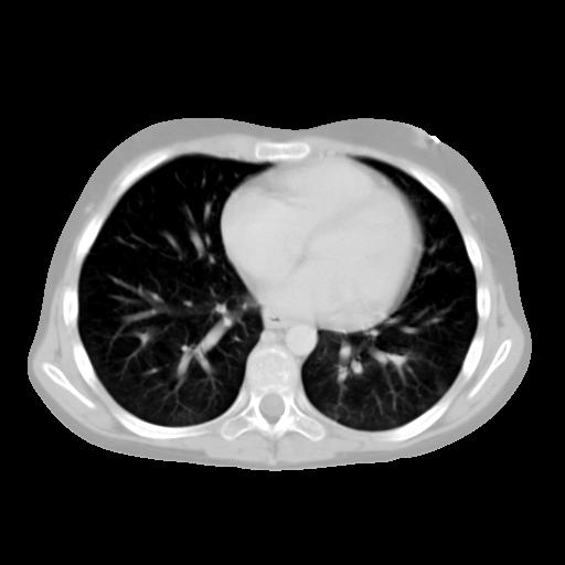
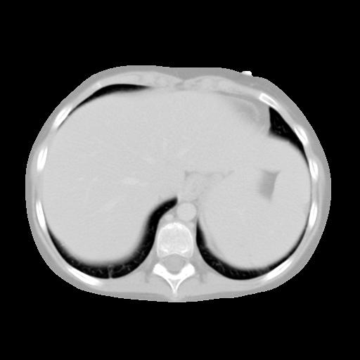
103 Segmentation of the Lungs: Results 103

104 Delineation of the Diaphragm Representation of the diaphragm using LLS: right-dome surface left-dome surface 104

105 Delineation of the Diaphragm Representation of the diaphragm using LLS and active contours: combined surface after applying active contour 105

106 Delineation of the Diaphragm Representation of the diaphragm using LLS and active contours: Segmented lungs and the diaphragm 106

107 Results: Diaphragm --- contours drawn by a radiologist --- contours obtained by the proposed methods 107

108 Results: Diaphragm Quantitative assessment: Number of CT exams: 11 (of six patients) Number of selected slices: 109 Average MDCP in 3D: 6.05 mm Average maximum Hausdorff distance in 3D: mm 108

109 Removal of the Thoracic Cavity 109

110 Delineation of the Pelvic Girdle Automatic detection of seed voxels using information related to the spinal canal, the vertebral column, and the peripheral fat boundary. 110

111 Delineation of the Pelvic Girdle Automatic segmentation performed using fuzzy mapping and opening-by-reconstruction (in 3D). 111

112 Results: Pelvic Girdle -- contours drawn by a radiologist -- contours obtained by the proposed methods 112

113 Results: Pelvic Girdle Quantitative assessment: Number of CT exams: 13 (of six patients) Number of selected slices: 277 Average MDCP in 3D: 0.53 mm Average maximum Hausdorff distance in 3D: 5.95 mm 113

114 Modeling the Upper Surface of the Pelvic Girdle Representation of the upper surface of the pelvic girdle using the LLS model and active contours: Linear least-squares model Refined pelvic surface 114

115 Removal of the Pelvic Cavity 115

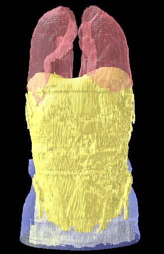
116 Results: Landmarks Identified 116

117 Application to the Segmentation of Neuroblastic Tumors Neuroblastoma Malignant tumor Originates along the sympathetic ganglia or in the adrenal medulla. Accounts for 8 10% of all childhood cancers. 65% of the tumors are located in the abdomen. Sympathetic Ganglia Pelvis Adrenal Medulla 117

118 CT Image of Neuroblastoma Abdominal tumors are most common: the worst prognosis. Generally heterogeneous, with a mixture of: calcification viable tumor necrosis necrosis (low density), viable tumor (medium density), calcification (high density). 118

119 Tumor Response to Therapy Tumor shrinks Intermediate density: active or viable tumor Low density: necrosis High density: calcified tissue April 2001 June 2001 September

120 Tumor mass enclosing the aorta: unresectable 120

121 Clinical and Image-based Analysis 121

122 Original CT volume Removal of external air, peripheral artifacts, and the skin layer Removal of the peripheral fat region Removal of the peripheral muscle Segmentation of the rib structure Segmentation of the vertebral column Segmentation of the spinal canal; removal of the vertebral column Delineation of the pelvic girdle; removal of the pelvic cavity Removal of the spinal canal Segmentation of the lungs Delineation of the diaphragm; removal of the thoracic cavity Fuzzy segmentation of the tumor; threshold Segmented tumor volume 122

123 Segmentation of the Tumor 1. A region within the tumor mass manually selected. 2. Region statistics, µ R and σ R, calculated. 3. Data volume mapped using fuzzy mapping function f M ( r) = exp 1 2 r µ R σ R 2 where r is an arbitrary pixel in the image. 123

124 Segmentation of the Tumor 4. The selected region is used as a region marker 5. Reconstruction performed to obtain graded connected components using fuzzy-mapped image as mask and the region marker 6. Image thresholded using R R T = µ + 0.5σ 124

125 Segmentation of Neuroblastoma: Homogeneous Tumor a b a. tumor segmented by a radiologist c d b. user-selected region marker c. result of openingby-reconstruction d. final result of segmentation 125

126 Segmentation of Neuroblastoma: Heterogeneous Tumor a c b d a. tumor segmented by a radiologist b. user-selected region marker c. result of openingby-reconstruction d. final result of segmentation 126

127 Segmentation of Neuroblastoma: Diffuse Tumor a b a. tumor segmented by a radiologist c d b. user-selected region marker c. result of openingby-reconstruction d. final result of segmentation 127

128 Result of Segmentation: Homogeneous Tumor Tumor segmented by a radiologist Initial result of tumor segmentation After removal of the thoracic cavity After removal of regions below the pelvic surface 128

129 Result of Segmentation: Heterogeneous Tumor Tumor segmented by a radiologist Initial result of tumor segmentation After removal of the thoracic cavity After removal of regions below the pelvic surface 129

130 Result of Segmentation: Diffuse Tumor Tumor segmented by a radiologist Initial result of tumor After removal of the segmentation thoracic cavity After removal of regions below the pelvic surface 130

131 Results 131

132 Results Effect of removal of the thoracic cavity: false-positive rate reduced by 8.3%, on the average, over 10 CT exams of four patients. Effect of removal of the vertebral column and the regions below the pelvic surface: false-positive rate reduced by 10.3%, on the average. True-positive rate: 82.1%, on the average. 132

133 Conclusion The proposed methods: separate the thoracic, abdominal, and pelvic cavities for further consideration; facilitate atlas-based and landmark-based approaches to segmentation of medical images; aid in reducing the false-positive error rate in the result of segmentation of tumors. 133

134 Future work Incorporation of other abdominal, thoracic, and pelvic landmarks. Extension of the methods to other imaging modalities. Implementation of competitive region growing for segmentation of multiple organs and tumors. Estimation of tissue composition in tumor mass using Gaussian mixture model. 134

135 Thank you This work is supported by a grant from the Natural Sciences and Engineering Research Council (NSERC) of Canada. We thank Hanford Deglint and Randy Vu for their contributions to this project.