Clustering Data That Resides on a Low-Dimensional Manifold in a High-Dimensional Measurement Space. Avinash Kak Purdue University

Transcription

1 Clustering Data That Resides on a Low-Dimensional Manifold in a High-Dimensional Measurement Space Avinash Kak Purdue University February 15, :37am An RVL Tutorial Presentation Originally presented in Fall 2008 Revised (minor) in February 2016 c 2016 Avinash Kak, Purdue University 1

2 CONTENTS Page PART I 4 1 Why Manifolds for Data Clustering and 5 Machine Learning? 2 Thinking of a Nonlinear Manifold as 18 a Collection of Hyperplanes 3 Understanding the Notions of Subspace 20 and Reconstruction Error 4 The Basic Algorithm for Data Clustering 23 on a Manifold by Minimizing the Reconstruction Error 5 Why a 2-Phase Approach to Clustering by 27 Minimization of Reconstruction Error? 6 Using Graph Partitioning to Merge Small 30 Clusters 7 Summary of the Overall Algorithm 37 8 The Perl Module 43 Algorithm::LinearManifoldDataClusterer Fail-First Bias of the Module Some Results Obtained with the Perl Module 53 Algorithm::LinearManifoldDataClusterer continued on next page... 2

3 CONTENTS (contd.) PART II Calculating Manifold-based Geodesic 63 Distances from Measurement-Space Distances 12 The ISOMAP Algorithm for Estimating the 68 the Geodesic Distance 13 Using MDS along with D M Distances to 70 Construct Lower-Dimensional Representation for the Data 14 Computational Issues Related to ISOMAP Dimensionality Reduction by Locally Linear 81 Embedding (LLE) 16 Estimating the Weights for Locally Linear 82 Embedding of the Measurement Space Data Points 17 Invariant Properties of the Reconstruction 87 Weights 18 Constructing a Low-Dimensional 89 Representation from the Reconstruction Weights 19 Some Examples of Dimensionality Reduction 93 with LLE 20 Acknowledgments 96 3

4 PART I: Clustering on Nonlinear Manifolds by Minimization of Reconstruction Error 4

5 1: Why Manifolds for Data Clustering and Machine Learning? If you are new to machine learning and data clustering on linear and nonlinear manifolds, your first question is likely to be: What is a manifold? A manifold is a space that is locally Euclidean. And a space is locally Euclidean if it allows for the points in a small neighborhood to be represented by, say, Cartesian coordinates and if the distances between the points in the neighborhood are given by the Euclidean metric. For example, the set of ALL points on the surface of a sphere does NOT constitute a Euclidean space. Nonetheless, if you confined your attention to a small enough neighborhood around a point, the space would seem to be locally Euclidean. [As you know, the ancients believed that the earth was flat.] 5

6 The surface of a sphere is a 2-dimensional manifold embedded in a 3-dimensional space. A plane in a 3-dimensional space is also a 2-dimensional manifold. You would think of the surface of a sphere as a nonlinear manifold, whereas a plane would be a linear manifold. However, note that any nonlinear manifold is locally a linear manifold. That is, given a sufficiently small neighborhood on a nonlinear manifold, you can always think of it as a locally flat surface. As to why we need machine learning and data clustering on manifolds, there exist many important applications in which the measured data resides on a nonlinear manifold. 6

7 For example, when you record images of a human face from different angles, all the image pixels taken together fall on a lowdimensional surface in a high-dimensional measurement space. The same is believed to be true for the satellite images of a land mass that are recorded with the sun at different angles with respect to the direction of the camera. Reducing the dimensionality of the sort of data mentioned above is critical to the proper functioning of downstream classification algorithms, and the most popular traditional method for dimensionality reduction is the Principal Components Analysis (PCA) algorithm. 7

8 However, using PCA is tantamount to passing a linear least-squares hyperplane through the surface on which the data actually resides. As to why that might be a bad thing to do, just imagine the consequences of assuming that your data falls on a straight line when, in reality, it falls on a strongly curving arc. [This is exactly what happens with PCA it gives you a linear manifold approximation to your data that may actually reside on a curved surface.] In the rest of this section, I ll provide a more phenomenological explanation for why certain kinds of data gives rise to shaped surfaces in the measurement space. Toward that end, consider the two-pixel images formed as shown in the next figure. We will assume that the object surface is Lambertian and that the object is lighted with focused illumination as shown. 8

9 x 1 x 2 Data on Manifolds Tutorial Orthographic Projection Camera Direction of Illumination We will record a sequence of images as the object surface is rotated vis-a-vis the illumination. We will assume that the pixel x 1 in each image is roughly a quarter of the width from the left edge of each image and the pixel x 2 about a quarter of the width from the right edge. We will further assume that the sequence of images is taken with the object rotated through all of 360 around the axis shown. 9

10 Because of Lambertian reflection, the two pixels in an image indexed i will be roughly as (x 1 ) i = Acosθ i (x 2 ) i = Bcos(θ i +45 ) where θ i is the angle between the surface normal at the object point that is imaged at pixel x 1 and the illumination vector and where we have assumed that the two panels on the object surface are at a 45 angle. So as the object is rotated, the image point in the 2D feature space formed by the pixels (x 1,x 2 ) will travel a trajectory as shown in the next figure. [Note that the beginning and the end points of the curve in the feature space are not shown as being the same because we may not expect the reflectance properties of the back of the object to be the same as those of the front. ] 10

11 A x 2 B x 1 The important point to note is that when the data points in a feature space are as structured as shown in the figure above, we cannot use Euclidean metric in that space as a measure of similarity. Two points, such as A and B marked in the figure, may have short Euclidean distance between them, yet they may correspond to patterns that are far apart from the standpoint of similarity. 11

12 The situation depicted in the figure on the previous slide can be described by saying that the patterns form a 1D manifold in an otherwise 2D feature space. That is, the patterns occupy a space that has, locally speaking, only 1 DOF. It would obviously be an error to use linear methods like those based on, say, PCA for data clustering in such cases. Let s now add one more motion to the object in the imaging setup shown on Slide 9. In addition to turning the object around its long axis, we will also rock it up and down at its back edge while not disturbing the front edge. The second motion is depicted in the next figure. Let s also now sample each image at three pixels, as shown in the next figure. 12

13 Orthographic Projection Camera Random Rocking Direction of Illumination x 1 Random Rotations x 3 x 2 Note again, the pixels do not correspond to fixed points on the object surface. Rather, they are three pixels of certain prespecified coordinates in the images. So each image will be now be represented by the following 3-vector: x i = x 1 x 2 x 3 13

14 We will assume that the data is generated by random rotations and random rocking motions of the object between successive image captures by the camera. Each image will now be one point is a 3-dimensional space. Since the brightness values at the pixels x 1 and x 3 will always be nearly the same, we will see a band-like spread in the (x 1,x 3 ) plane. These images will now form a 2D manifold in the 3D (x 1,x 2,x 3 ) space as shown in the figure below. x 2 x 3 x 1 14

15 Another example of the data points being distributed on a manifold is shown in the figure shown below. This figure represents three dimensional data that is sampled from a two-dimensional manifold. [A manifold s dimensionality is determined by asking the question: How many independent basis vectors do I need to represent a point inside a local neighborhood on the surface of the manifold?] 15

16 To underscore the fact that using straightline Euclidean distance metric makes no sense when data resides on a manifold, the distribution presented in the previous figure shows two points that are connected by a straight-line distance and a geodesic. The straight-line distance could lead to the wrong conclusion that the points represent similar patterns, but the geodesic distance tells us that those two points correspond to two very different patterns. In general, when data resides on a manifold in an otherwise higher dimensional feature space, we want to compare pattern similarity and establish neighborhoods by measuring geodesic distances between the points. 16

17 Again, in our discussion, a manifold will be a lower-dimensional surface in a higherdimensional space. And, the geodesic distance between two points on a given manifold is the shortest distance between the two points on the manifold. As you know, the shortest distance between any two points on the surface of the earth is along the great circle that passes through those points. So the geodesic distances on the earth are along the great circles. 17

18 2: Thinking of a Nonlinear Manifold as a Collection of Hyperplanes Since a nonlinear manifold is locally linear, we can think of each data cluster on a nonlinear manifold as falling on a locally linear portion of the manifold, meaning on a hyperplane. So our goal should be to find find a set of hyperplanes that best describes the data, with each hyperplane derived from a local data cluster. This would be like constructing a piecewise linear approximation to data that falls on a curve as opposed to constructing a single straight line approximation to all of the data. 18

19 So whereas the frequently used PCA algorithm gives you a single hyperplane approximation to all your data, what we want to do is to calculate a set of hyperplane approximations, with each hyperplane derived by applying the PCA algorithm locally to a data cluster. That brings us to the problem of how to actually discover the best set of hyperplane approximations to the data. What is probably the most popular algorithm today for that purpose is based on the following key idea: Given a set of subspaces to which a data element can be assigned, you assign it to that subspace for which the reconstruction error is the least. But what do we mean by a subspace and what is reconstruction error? These notions are explained in the next section. 19

20 3: Understanding the Notions of Subspace and Reconstruction Error To understand the notions of subspace and reconstruction-error, let s revisit the traditional approach of dimensionality reduction by the PCA algorithm. The PCA algorithm consists of: (1) Subtracting from each data element the global mean of the data; (2) Calculating the covariance matrix of the data; (3) Carrying out an eigendecomposition of the covariance matrix and ordering the eigenvectors according to decreasing values of the corresponding eigenvalues; (4) Forming a subspace by discarding the trailing eigenvectors whose corresponding eigenvalues are relatively small; and, finally, (5) projecting all the data elements into the subspace so formed. 20

21 The error incurred in representing a data element by its projection into the subspace is known as the reconstruction error. This error is the projection of the data element into the space spanned by the discarded trailing eigenvectors. In linear-manifold based machine learning, instead of constructing a single subspace in the manner described above, we construct a set of subspaces, one for each data cluster on the nonlinear manifold. After the subspaces have been constructed, a data element is assigned to that subspace for which the reconstruction error is the least. On the face of it, this sounds like a chickenand-egg sort of a problem: You need to have already clustered the data in order to construct the subspaces at different places on the manifold so that you can figure out which cluster to place a data element in. 21

22 Such problems, when they do possess a solution, are best tackled through iterative algorithms in which you start with a guess for the final solution, you rearrange the measured data on the basis of the guess, and you then use the new arrangement of the data to refine the guess. Subsequently, you iterate through the second and the third steps until you do not see any discernible changes in the new arrangements of the data. This forms the basis of the clustering algorithm that is described under Phase 1 in the section that follows. This algorithm was first proposed in the article Dimension Reduction by Local Principal Component Analysis by Kambhatla and Leen that appeared in the journal Neural Computation in

23 4. The Basic Algorithm for Data Clustering on a Manifold by Minimizing the Reconstruction Error Let s say we have N data points in a multidimensional space: X = {x i i = 1,2,...,N } Assume for a moment that this data has somehow been partitioned into K disjoint clusters: X = X 1 X 2... X K X i X j = 0 i j Let S = { S i i = 1,2,...,K } represent a set of K subspaces that correspond to the clusters X i,i = 1,K. 23

24 The subspace S i is constructed by first calculating the mean and the covariance of the data points in X i : C i = 1 N i N i 1 (x j m i )(x j m i ) T, x j X i j=0 where m i is the cluster mean as given by m i = 1 N i N i 1 i=0 x j, x j X i For constructing the subspace S i, we carry out an eigendecomposition of the covariance matrix C i and use the P leading eigenvectors for defining the local coordinate frame for the subspace S i. We will use the notation WP i to denote the matrix formed by the P leading eigenvectors of C i and the notation W i P to denote the remaining (meaning the trailing) eigenvectors of C i. 24

25 For any data element x k X, the error in representing it by its projection in the subspace S i is given by e = W i P T (x k m i ) We can write the following form for the square-magnitude of this error: d 2 err (x k,s i ) = e 2 = e T e = (x k m i ) T W i P W i T P (x k m i ) As shown on the next slide, we will now re-partition X into K clusters on the basis of the minimization of the error function shown above. 25

26 Using the primed notation for the new clusters, we seek X = X 1 X 2... X M with X i X j = 0 i j such that X i = { } x j derr (x j,s i ) < d err (x j,s k ),k i We keep track of the reconstruction error incurred in assigning each data element to its cluster and characterize each iteration of the algorithm on the basis of the sum of these errors. We stop the iterations when the change in these summed errors falls below a threshold. 26

27 5. Why a 2-Phase Approach to Clustering by Minimization of the Reconstruction Error? Unfortunately, experiments show that the algorithm as proposed by Kambhatla and Leen is much too sensitive to how the clusters are seeded initially. One possible way to get around this limitation of the algorithm is by using a two phased approach as described below. In the first phase, you construct clusters but by looking for more clusters than are actually present in the data. This increases the odds that each original cluster will be visited by one or more of the randomly selected seeds at the beginning. 27

28 Subsequently, one can merge the clusters that belong together in order to form the final clusters. That work can be done in the second phase. For the cluster merging operation in the second phase, we can model the clusters as the nodes of a graph in which the weight given to an edge connecting a pair of nodes measures the similarity between the two clusters corresponding to the two nodes. Subsequently, as described in Section 6, we can use a modern graph partitioning algorithm to merge the most similar nodes in our quest to partition the data into the desired number of clusters. These algorithms require us to define pairwise similarity between the nodes of the graph. 28

29 With regard to the pairwise similarity matrix required by a graph partitioning algorithm, we know that the smaller the overall reconstruction error when all of the data elements in one cluster are projected into the other s subspace and vice versa, the greater the similarity between two clusters. Additionally, the smaller the distance between the mean vectors of the clusters, the greater the similarity between two clusters. The overall similarity between a pair of clusters is a combination of these two similarity measures. 29

30 6. Using Graph Partitioning for Merging Small Clusters Before reading this section, you might want to go through the very readable survey paper A Tutorial on Spectral Clustering by Luxburg that appeared in the journal Statistics and Computing in It is available for free download on the web. As to the reason for why we need graph partitioning, as mentioned earlier, a plain vanilla iterative implementation of the logic of Section 4 results in clustering that is too sensitive to how the clusters are initialized at the beginning of the first iteration. [As the reader would recall, if you expect to see N clusters in your data, the clusters are initialized by picking N data elements randomly to serve as cluster centers and then partitioning the rest of the data on the basis of the least Euclidean distance from the randomly selected cluster centers.] 30

31 As a hedge against this sensitivity to how the clusters are initialized with random selection of cluster centers, we go for the 2-phased approach described in Section 4. If we expect to see, say, K clusters in the data, in the first phase we actually look for M K clusters with M > 1 with the expectation that the random seeding of the M K clusters will increase the odds that every one of the actual K will be seen by at least one seed. So our goal in Phase 2 is to apply a merging step to the M K clusters returned by Phase 1 so that we end up with just K clusters we expect to see in the data. This is exactly the problem that is solved by the algorithms described in the article by Luxburg mentioned at the beginning of this section. 31

32 What we want to do is to represent all of the clusters that are output by Phase 1 as the nodes of a graph G = (V,E) in which the set of nodes V = {v 1,v 2,...,v n } stands for the clusters. Given a graph G, we associate with each edge {v i,v j } a non-negative weight w i,j that tells us how similar node v i is to node v j, meaning how similar the cluster indexed i is to the cluster indexed j. In our context, we can base cluster-to-cluster similarity on two considerations that are equally relevant to the problem at hand: one based on the reconstruction error and the other based on the distance between the means to the two clusters as explained on the next side. 32

33 We say that smaller the overall reconstruction error when all of the data elements in one cluster are projected into the other s subspace and vice versa, the greater the similarity between two clusters. And we say that the smaller the distance between the mean vectors of the clusters, the greater the similarity between two clusters. The overall similarity between a pair of clusters can then be a combination of these two similarity measures. Should it happen that w i,j = 0, that means that the nodes v i and v j are not connected. The matrix formed by these weights, denoted W, is called the similarity matrix for the graph. (This matrix is also known as the weighted adjacency matrix for a graph.) 33

34 We associate with each node v i a degree d i defined by d i = n j=1 w i,j. We place all node degrees in an n n diagonal matrix D, called the degree matrix, whose i th element is d i. The algorithms described in Luxburg s article partition a graph G into disjoint collections of nodes so that the nodes in each collection are maximally similar, while, at the same time, the collections are maximally dissimilar from one another. More specifically, we want the total weight of the edges in each collection to be as large as it can be, while, at the same time, we want the total weight of the edges that are between the collections to be as small as it can be. All graph spectral clustering algorithms use the notion of a graph Laplacian. 34

35 Given the similarity matrix W and the degree matrix D as defined above, the Laplacian of a graph G is defined as L = D W. The Laplacian of a graph as defined above has some very interesting properties: (1) It is symmetric and positive-definite; (2) Its smallest eigenvalue is always 0 and the corresponding eigenvector a unit vector, meaning a vector all of whose elements are 1 s; and (3) All of its eigenvalues are non-negative. (See Luxburg s paper for proofs.) My personal favorite algorithm for graph partitioning is the Shi-Malik algorithm. It is based on the symmetric normalized Laplacian defined as L sym = D 1 2(D W)D 1 2. Just like the Laplacian L, L sym also possesses some very interesting properties that you ll see listed in Luxburg s article. 35

36 If we use W(G 1,G 2 ) = u G 1,v G 2 w u,v to denote the total similarity weight in the edges that connect any of the nodes in G 1 with any of the nodes in G 2, and if we use vol(g i ) = v G i d v to denote the total similarity weight emanating from all the nodes in the partition G i, the Shi-Malik algorithm can be used to optimally bipartition G using the eigenvector of L sym that corresponds to the second smallest eigenvalue. This bipartition minimizes the normalized graph cut: Ncut(H, H) = W(H, H vol(h) + W(H, H vol( H) Finer partitions of a graph can be created by invoking the Shi-Malik algorithm recursively. 36

37 7. Summary of the Overall Algorithm I will now present a summary of the two phases of the algorithm implemented in my Perl module that is presented in the next section. In what follows, an important role is played by what we will later refer to as the constructor parameter cluster search multiplier. It is only when the integer value given to this parameter is greater than 1 that Phase 2 of the algorithm kicks in. In this summary presentation, this parameter will be denoted M. We will also use the parameter P to denote the dimensionality of the manifold. PHASE 1: In this phase, we invoke the algorithm described in Section 4 to partition the data into clusters. The number of clusters formed is the product of K, which is the number of clusters expected by the user, and the parameter M mentioned above to induce over clustering of the data. 37

38 Step 1: Randomly choose M K data elements to serve as the seeds for that many clusters. Step 2: Construct initial M K clusters by assigning each data element to that cluster whose seed it is closest to. Step 3: Calculate the mean and the covariance matrix for each of the M K clusters and carry out an eigendecomposition of the covariance matrix. Order the eigenvectors in decreasing order of the corresponding eigenvalues. The first P eigenvectors define the subspace for that cluster. Use the space spanned by the remaining eigenvectors we refer to them as the trailing eigenvectors for calculating the reconstruction error. 38

39 Step 4: Taking into account the mean associated with each cluster, re-cluster the entire data set on the basis of the least reconstruction error. That is, assign each data element to that subspace for which it has the smallest reconstruction error. Calculate the total reconstruction error associated with all the data elements. (See the definition of the reconstruction error in Section 4.) Step 5: Stop iterating if the change in the total reconstruction error from the previous iteration to the current iteration is less than the value specified by the constructor parameter delta reconstruction error. Otherwise, go back to Step 3. PHASE 2: This phase of the algorithm uses graph partitioning to merge the M K clusters back into the K clusters you expect to see in your data. 39

40 Since the algorithm whose steps are presented below is invoked recursively, let s assume that we have N clusters that need to be merged by invoking the Shi-Malik spectral clustering algorithm as described below: Step 1: Form a graph whose N nodes represent the N clusters. (For the very first invocation of this step, we have N = M K.) Step 2: Construct an N N similarity matrix for the graph. The (i,j)-th element of this matrix is the similarity between the clusters indexed i and j. Calculate this similarity using two criteria: (1) The total reconstruction error when the data elements in the cluster indexed j are projected into the subspace for the cluster indexed i and vice versa. And (2) The distance between the mean vectors associated with the two clusters. 40

41 Step 3: Calculate the symmetric normalized Laplacian of the similarity matrix. We use A to denote the symmetric normalized Laplacian. Step 4: Do eigendecomposition of the A matrix and choose the eigenvector corresponding to the second smallest eigenvalue for bipartitioning the graph on the basis of the sign of the values in the eigenvector. Step 5: If the bipartition of the previous step yields one-versus-the-rest kind of a partition, add the one cluster to the output list of clusters and invoke graph partitioning recursively on the rest by going back to Step 1. On the other hand, if the cardinality of both the partitions returned by Step 4 exceeds 1, invoke graph partitioning recursively on both partitions. Stop when the list of clusters in the output list equals K. 41

42 Step 6: In general, the K clusters obtained by recursive graph partitioning will not cover all of the data. So, for the final step, assign each data element not covered by the K clusters to that cluster for which its reconstruction error is the least. The 2-Phase algorithm described in this section is implemented in the Perl module described in the next section. 42

43 8. The Perl Module Algorithm::LinearManifoldDataClusterer-1.01 The goal of this section is to introduce the reader to some of the more important functions in my Perl module Algorithm::LinearManifoldDataClusterer that can be downloaded from 0/lib/Algorithm/LinearManifoldDataClusterer.pm Please read the documentation at the CPAN site for the API of this software package. [The URL shown above is supposed to be one continuous string. You can also just do a Google search on the string Algorithm::LinearManifoldDataClusterer and go to Version 1.01 when you get to the CPAN page for the module.] 43

44 The module defines two classes: LinearMani folddataclusterer and DataGenerator, the former for clustering data on nonlinear manifolds by assuming to be piecewise linear and the latter for generating synthetic data for experimenting with the clusterer. The data file presented to the module must be in CSV format and each record in the file must include a symbolic tag for the record. Here is an example of what a typical data file would look like: d_161, , , a_59, , , a_225, , , a_203, , , What you see in the first column d_161, a_59, a_225>, a_203 are the symbolic tags associated with four 3-dimensional data records. 44

45 The module also expects that you will supply a mask that informs the module as to which columns of the numerical data it should use for clustering. An example of a mask when the first column contains the symbolic tag and the next three columns the numerical data would be N111. In order to use the module for clustering, you must first create an instance of the clusterer though a call like this: my $clusterer = Algorithm::LinearManifoldDataClusterer->new( datafile => $datafile, mask => $mask, K=> 3, P=> 2, max_iterations => 15, cluster_search_multiplier => 2, delta_reconstruction_error => 0.001, terminal_output => 1, visualize_each_iteration => 1, show_hidden_in_3d_plots => 1, make_png_for_each_iteration => 1, ); 45

46 In the constructor call shown on the previous slide, the parameter K specifies the number of clusters you expect to find in your data and the parameter P is the dimensionality of the manifold on which the data resides. The parameter cluster_search_ multiplier is for increasing the odds that the random seeds chosen initially for clustering will populate all the clusters. Set this parameter to a low number like 2 or 3. The parameter max_iterations places a hard limit on the number of iterations that the algorithm is allowed. The actual number of iterations is controlled by the parameter delta_reconstruction_error. The iterations stop when the change in the total reconstruction error from one iteration to the next is smaller than the value specified by delta_reconstruction_error. After the constructor call, you can read in the data and initiate clustering, as shown on the next slide. 46

47 You get the module to read the data for clustering through the following call: $clusterer->get_data_from_csv(); Now you can invoke linear manifold clustering by: my $clusters = $clusterer->linear_manifold_clusterer(); The value returned by this call is a reference to an array of anonymous arrays, with each anonymous array holding one cluster. If you wish, you can have the module write the clusters to individual files by the following call: $clusterer->write_clusters_to_files($clusters); 47

48 If you want to see how the reconstruction error changes with the iterations, you can make the call: $clusterer-> \ display_reconstruction_errors_as_a_function_of_iterations(); When your data is 3-dimensional and when the clusters reside on a surface that is more or less spherical, you can visualize the clusters by calling $clusterer-> \ visualize_clusters_on_sphere( final clustering, $clusters); where the first argument is a label to be displayed in the 3D plot and the second argument the value returned by calling linear_ manifold_clusterer(). 48

49 9. Fail-First Bias of the Module As you would expect for all such iterative algorithms, the module carries no theoretical guarantee that it will give you correct results. But what does that mean? Suppose you create synthetic data that consists of Gaussian looking disjoint clusters on the surface of a sphere, would the module always succeed in separating out the clusters? The module carries no guarantees to that effect especially considering that Phase 1 of the algorithm is sensitive to how the clusters are seeded at the beginning. 49

50 Although this sensitivity is mitigated by the cluster merging step when greater-than-1 value is given to the constructor option cluster_search_multiplier, a plain vanilla implementation of the steps in Phase 1 and Phase 2 would nonetheless carry significant risk that you ll end up with incorrect clustering results. To further reduce this risk, the module has been programmed so that it terminates immediately if it suspects that the cluster solution being developed is unlikely to be fruitful. The heuristics used for such terminations are conservative since the cost of termination is only that the user will have to run the code again, which at worst only carries an element of annoyance with it. 50

51 The three Fail First heuristics currently programmed into the module are based on simple unimodality testing, testing for congruent clusters, and testing for dominant cluster support in the final stage of the recursive invocation of the graph partitioning step. The unimodality testing is as elementary as it can be it only checks for the number of data samples within a certain radius of the mean in relation to the total number of data samples in the cluster. When the program terminates under such conditions, it prints out the following message in your terminal window: Bailing out! 51

52 Given the very simple nature of testing that is carried for the Fail First bias, do not be surprised if the results you get for your data simply look wrong. If most runs of the module produce wrong results for your application, that means that the module logic needs to be strengthened further. The author of this module would love to hear from you if that is the case. 52

53 10. Some Results Obtained with the Perl Module Algorithm::LinearManifoldDataClusterer This section presents some results obtained with the Algorithm::LinearManifoldDataClusterer module. In this tutorial, I will show manifold based clustering results obtained with the first two of the following four canned scripts that you will find in the examples directory of the module: example1.pl example2.pl example3.pl example4.pl These scripts use the following data files that are also in the examples directory: 3_clusters_on_a_sphere_498_samples.csv 3_clusters_on_a_sphere_3000_samples.csv 4_clusters_on_a_sphere_1000_samples.csv (used in example1.pl and example4.pl) (used in example2.pl) (used in example3.pl) 53

54 With regard to the data files listed on the previous slide, even though the first two of these files both contain exactly three clusters, the clusters look very different in the two data files. The clusters are much more spread out in 3_clusters_on_a_sphere_3000_ samples.csv. The code in example4.pl is special because it shows how you can call the auto_retry_ clusterer() method of the module for automatic repeated invocations of the clustering program until success is achieved. [The value of the constructor parameter cluster search multiplier is set to 1 in example4.pl, implying that when you execute example4.pl you will not be invoking Phase 2 of the algorithm. You might wish to change the value given to this parameter to see how it affects the number of attempts needed to achieve success.] 54

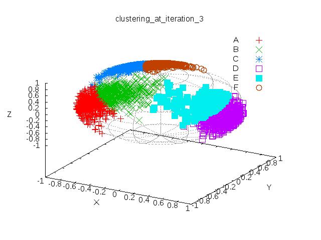
55 We will start with the results obtained with the script example1.pl. We use the following constructor parameters in this script: K => 3, # number of clusters P => 2, # manifold dimensionality max_iterations => 15, cluster_search_multiplier => 2, delta_reconstruction_error => 0.001, Note, in particular, the value of 2 given to the parameter cluster search multiplier. This implies that Phase 1 of the algorithm will look for 6 clusters. Subsequently, in Phase 2, these would go through a merging step to yield the final 3 clusters. The next four figures show: (1) The initial clustering of the data at the outset of the iterations when the cluster centers are chosen randomly; (2) Clustering results after 3 iterations of the Phase 1 algorithm; (3) Clustering achieved after the merge operation of Section 5; and (4) The final result. 55

56 56

57 57

58 The results shown next were obtained with the example2.pl in the examples directory of the module. As mentioned previously, this script uses the data that is in the file 3 clusters on a sphere 3000 samples.csv. The example2.pl script uses the following constructor parameters: K => 3, # number of clusters P => 2, # manifold dimensionality max_iterations => 15, cluster_search_multiplier => 2, delta_reconstruction_error => 0.012, which, except for the value given to delta reconstruction error, are the same as for example1.pl. [IMPORTANT: In general, the value you would need to give to delta reconstruction error would be larger, the larger number of data samples that need to be clustered.] In this case, we have 3000 samples. 58

59 Since the value given to the parameter cluster search multiplier is 2, this implies that Phase 1 of the algorithm will look for 6 clusters. Subsequently, in Phase 2, these would go through a merging step to yield the final 3 clusters. The next four figures show: (1) The initial clustering of the data at the outset of the iterations when the cluster centers are chosen randomly; (2) Clustering results after 3 iterations of the Phase 1 algorithm; (3) Clustering achieved after the merge operation of Section 5; and (4) The final result. 59

60 60

61 61

62 Part II: A Review of the ISOMAP and LLE Algorithms Part II of this tutorial is based on (1) A Global Geometric Framework for Nonlinear Dimensionality Reduction, by Tenenbaum, de Silva, and Lengford, Science, Dec. 2000; (2) Nonlinear Dimensionality Reduction by Locally Linear Embedding, by Roweis and Saul, Science, Dec. 2000; and (3) other related publications by these authors. 62

63 11: Calculating Manifold-based Geodesic Distances from Measurement-Space Distances We will now address the following problem regarding the measurement of distances on a manifold: How to calculate the geodesic distances between any two given points on the manifold? Theoretically, the problem can be stated in the following manner: Let M be a d-dimensional manifold in the Euclidean space R D. Let s now define a distance metric between any two points x and y on the manifold by d M ( x, y) = inf γ { length(γ) } 63

64 where γ varies over the set of arcs that connect x and y on the manifold. To refresh your memory, infimum of a set means to return an element that stands for the greatest lower bound vis-a-vis all the elements in the set. In our case, the set consists of the length values associated with all the arcs that connect x and y. The infimum returns the smallest of these length values. Our goal is to estimate d M ( x, y) given only the set of points { x i } R D. We obviously have the ability to compute the pairwise Euclidean distances x, y in R D. We can use the fact that when the data points are very close together according to, say, the Euclidean metric, they are also likely to be close together on the manifold (if one is present in the feature space). 64

65 It is only the medium to large Euclidean distances that cannot be trusted when the data points reside on a manifold. So we can make a graph of all of the points in a feature space in which two points will be directly connected only when the Euclidean distance between them is very small. To capture this intuition, we define a graph G = {V,E} where the set V is the same as the set of data points { x i } and in which { x i, x j } E provided x i, x j is below some threshold. 65

66 We next define the following two metrics on the set of measured data points. For every x and y in the set { x i }, we define: d G ( x, y) = d S ( x, y) = min( x 0 x x p 1 x p ) P min(d M (x 0,x 1 ) d M (x p 1,x p )) P where the path P = ( x 0 = x, x 1, x 2,... x p = y) varies over all the paths along the edges of the graph G. As previously mentioned, our real goal is to estimate d M ( x, y). We want to be able to show that d G d M. We will establish this approximation by first demonstrating that d M d S and then that d S d G. 66

67 To establish these approximations, we will use the following inequalities: d M ( x, y) d S ( x, y) d G ( x, y) d S ( x, y) The first follows from the triangle inequality for the metric d M. The second inequality holds because the the Euclidean distances x i x i+1 are smaller than the arc-length distances d M ( x i, x i+1 ). The proof of the approximation d M d G is based on demonstrating that d S is not too much larger than d M and that d G is not too much smaller than d S. 67

68 12: The ISOMAP Algorithm for Estimating the Geodesic Distances The ISOMAP algorithm can be used to estimate the geodesic distances d M ( x, y) on a lower-dimensional manifold that is inside a higher-dimensional Euclidean measurement space R D. ISOMAP consists of the following steps: Construct Neighborhood Graph: Define a graph G over all the set { x i } of all data points in the underlying D-dimensional features space R D by connecting the points x and y if the Euclidean distance x y is smaller than a pre-specified ǫ (for ǫ-isomap). In graph G, set edge lengths equal to x y. 68

69 Compute Shortest Paths: Use Floyd s algorithm for computing the shortest pairwise distances in the graph G: Initialize d G (x,y) = x y if {x,y} is an edge in in graph G. Otherwise set d G (x,y) =. Next, for each node z {x i }, replace all entries d G (x,y) by min{d G (x,y), d G (x,z)+ d G (z,y)}. The matrix of final values D G = {d G (x,y)} will contain the shortest path distances between all pairs of nodes in G. Construct d-dimensional embedding: Now use classical MDS (Multidimensional Scaling) to the matrix of graph distances D G and thus construct an embedding in a d-dimensional Euclidean space Y that best preserves the manifold s estimated intrinsic geometry. 69

70 13: Using MDS along with D M Distances to Construct Lower-Dimensional Representation for the Data MDS finds a set of vectors that span a lower d-dimensional space such that the matrix of pairwise Euclidean distances between them in this new space corresponds as closely as possible to the similarities expressed by the manifold distances d M (x,y). Let this new d-dimensional space be represented by R d. Our goal is to map the dataset {x i } from the measurement Euclidean space R D into a new Euclidean space R d. 70

71 For convenience of notation, let x and y represent two arbitrary points in R D and also the corresponding points in in the target space R d. Our goal is to find the d basis vector for R d such that following cost function is minimized: E = D M D R d F where D R d( x, y) is the Euclidean distance between mapped points x and y and where F is the Frobenius norm of a matrix. Recall that for N measured data points in R D, both D M and D R d will be N N. [For a matrix A, its Frobenius norm is given by A F = i,j A ij 2 ] 71

72 In MDS algorithms, it is more common to minimize the normalized E = D M D R d F D M F Quantitative psychologists refer to this normalized form as stress. A classical example of MDS is to start with a matrix of pairwise distances between a set of cities and to then ask the computer to situate the cities as points on a plane so that visual placement of the cities would be in proportion to the inter-city distances. 72

73 For algebraic minimization of the cost function, the cost function is expressed as E = τ(d M ) τ(d R d) F where the τ operator coverts the distances to inner products. It can be shown that the solution to the above minimization consists of the using the largest d eigenvectors of the sampled τ(d M ) (or, equivalently, the estimated approximation τ(d G )) as the basis vectors for the reduced dimensionality representation of R d. The intrinsic dimensionality of a feature space is found by creating the reduced dimensionality mappings to R d for different values of d and retaining that value for d for which the residual E more or less the same as d is increased further. 73

74 When ISOMAP is applied to the synthetic Swiss roll data shown in the figure on Slide 15, we get the plot shown by the filled circles in the upper right-hand plate of the next figure that is also from the publication by Tenenbaum et al. As you can see, when d = 2, E goes to zero, as it should. The other curve in the same plate is for PCA. For curiosity s sake, the graph constructed by ISOMAP from the Swiss roll data is shown in the figure on the next slide. 74

75 In summary, ISOMAP creates a low-dimensional Euclidean representation from a measurement space in which the data resides on a manifold surface which could be a folded or a twisted surface. The other plots in the figure on the previous slide are for the other datasets for which Tenenbaum et al. have demonstrated the power of the ISOMAP algorithm for dimensionality reduction. 75

76 Tenenbaum et al. also experimented with a dataset consisting of images of a human head (a statue head). The images were recorded with three parameters, left-to-right orientation of the head, topto-bottom orientation of the head, and by changing the direction of illumination from left to right. Some images from the dataset are shown in the figure below. One can claim that even when you represent the images by vectors in R 4096, the dataset has only three DOF intrinsically. This is borne out by the output of ISOMAP shown in the upper-left of the plots on Slide

77 Another experiment by Tenenbaum et al. involved a dataset consisting of images of a human hand with two intrinsic degrees of freedom: one created by the rotation of the wrist and other created by the unfolding of the figures. The measurement space in this case is again R Some of the images in the dataset are shown in the figure below. The lower-left plate in the plots on Slide 74 corresponds to this dataset. 77

78 Another experiment carried out by Tenenbaum et al. used 1000 images of handwritten 2 s, as shown in the figure below. Two most significant features of how most humans write 2 s are referred to as the bottom loop articulation and the top arch articulation. The authors say they did not expect a constant low-dimensionality to hold over the entire dataset. 78

79 14: Computational Issues Related to ISOMAP ISOMAP calculation is nonlinear because it requires minimization of a cost function an obvious disadvantage vis-a-vis linear methods like PCA that are simple to implement. In general, it would require much trial and error to determine the best thresholds to use on the pairwise distances D( x, y) in the measurement space. Recall that when we construct a graph from the data points, we consider two nodes directly connected when the Euclidean distance between them is below a threshold. 79

80 ISOMAP assumes that the same distance threshold would apply everywhere in the underlying high-dimensional measurement space R D. ISOMAP also assumes implicitly that the same manifold would be a good fit for all of the measured data. 80

81 15: Dimensionality Reduction by Locally Linear Embedding (LLE) This is also a nonlinear approach, but does not require a global minimization of a cost function. LLE is based on the following two notions: When data resides on a manifold, any single data vector can be expressed as a linear combination of its K closest neighbors using a coefficient matrix whose rank is less than the dimensionality of the measurement space R D. The reconstruction coefficients discovered in expressing a data point in terms of its neighbors on the manifold can then be used directly to construct a lowdimensional Euclidean representation of the original measured data. 81

82 16: Estimating the Weights for Locally Linear Embedding of the Measurement Space Data Points Let x i be the i th data point in the measurement space R D and let { x j j = 1...K} be its K closest neighbors according to the Euclidean metric for R D, as depicted in the figure below. x 2 x i x 3 x 1 82

83 The fact that a data point can be expressed as a linear combination of its K closest neighbors can be expressed as x i = j w ij x j The equality in the above relationship is predicated on the assumption that the K closest data points are sufficiently linearly independent in a coordinate frame that is local to the manifold at x i. In order to discover the nature of linear dependency between the data point x i on the manifold and its K closest neighbors, it would be more sensible to minimize the following cost function: E i = x i j w ij x j 2 83

84 Since we will be performing the same calculations each measured data point x i, in the rest of the discussion we will drop the suffix i and let x stand for any arbitrary data point on the manifold. So for a given x, we want to find the best weight vector w = (w 1,...,w K ) that would minimize E( w) = x j w j x j 2 In the LLE algorithm, the weights w are found subject to the condition that jw j = 1. This constraint a sum-to-one constraint is merely a normalization constraint that expresses the fact that we want the proportions contributed by each of the K neighbors to any given data point to add up to one. 84

85 We now re-express the cost function at a given measured point x as E( w) = x j w j x j 2 = j w j ( x x j ) 2 where the second equality follows from the sum-to-unity constraint on the weights w j at all measured data points. Let s now define a local covariance at the data point x by C jk = ( x x j ) T ( x x k ) The local covariance matrix C is obviously an K K matrix whose (j,k) th element is given by inner product of the Euclidean distance between x and x j, on the one hand, and the distance x and x k, on the other. 85

86 In terms of the local covariance matrix, we can write for the cost function at a given measured data point x: E = j,k w j w k C jk Minimization of the above cost function subject to the constraint jw j = 1 using the method of Lagrange multipliers gives us the following solution for the coefficients w j at a given measured data point: w j = kc 1 jk i jc 1 ij 86

87 17: Invariant Properties of the Reconstruction Weights The reconstruction weights, as represented by the matrix W of the coefficients at each measured data point x, are invariant to the rotations of the measurement space. This follows from the fact that the scalar products that form the elements are of the local covariance matrix involve products of Euclidean distances in a small neighborhood around each data point. Those distances are not altered by rotating the entire manifold. The reconstruction weights are also invariant to the translations of the measurement space. This is a consequence of the sumto-one constraint on the weights. 87

88 We can therefore say that the reconstruction weights characterize the intrinsic geometrical properties in each neighborhood, as opposed to properties that depend on a particular frame of reference. 88

89 18: Constructing a Low-Dimensional Representation from the Reconstruction Weights The low-dimensional reconstruction is based on the idea we should use the same reconstruction weights that we calculated on the manifold that is, the weight represented by the vector w at each data point to reconstruct the measured data point in a low dimensional space. Let the low-dimensional representation of each measured data point x i be y i. LLE is founded on the notion that the previously computed reconstruction weights will suffice for constructing a representation of each y i in terms of its K nearest neighbors. 89

90 That is, we place our faith in the following equality in the to-be-constructed lowdimensional space: y i = j w ij y j But, of course, so far we do not know what these vectors y i are. So far we only know how they should be related. We now state the following mathematical problem: Considering together all the measured data points, find the best d-dimensional vectors y i for which the following global cost function is minimized Φ = i y i j w ij y j 2 If we assume that we have a total of N measured data points, we need to find N low-dimensional vector y i by solving the above minimization. 90

91 The form shown above can be re-expressed as Φ = i where j M ij y T i y j M ij = δ ij w ij w ji + k w ki w kj where δ ij is 1 when i = j and 0 otherwise. As it is, the above minimization is ill-posed unless the following two constraints are also used. We eliminate one degree of freedom in specifying the origin of the low-dimensional space by specifying that all of the new N vectors y i taken together be centered at the origin: i y i = 0 91

92 We require that the embedding vectors have unit variance with outer products that satisfy: 1 N i y i y T i = I where I is a d d identity matrix. The minimization problem is solved by computing the trailing d+1 eigenvectors of the M matrix and then discarding the last. The remaining d eigenvectors are the solution we are looking for. Each eigenvector has N components. When we arrange these eigenvectors in the form of a d N matrix, the column vectors of the matrix are the N vectors y i we are looking for. Recall N is the total number of measured data points. 92

93 19: Some Examples of Dimensionality Reduction with LLE In the example shown in the figure below, the measured data consists of 600 samples taken from an Swiss roll manifold. The calculations for mapping the measured data to a two-dimensional space was carried out with K = 12. That is, the local intrinsic geometry at each data point was calculated from the 12 nearest neighbors. 93

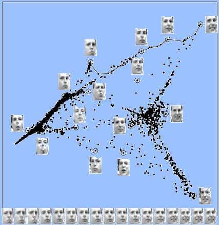
94 The next example was constructed from 2000 images (N = 2000) of the same face, with each image represented by a array of pixels. Therefore, the dimensionality of the measurement space is 560. The parameter K was again set to 12 for determining the intrinsic geometry at each 560 dimensional data point. The figure shows a 2-dimensional embeddings constructed from the data. Representative faces are shown next to circled points. The faces at the bottom correspond to the solid trajectory in the upper right portion of the figure. 94

95 95