COMP3421. Global Lighting Part 2: Radiosity

Transcription

1 COMP3421 Global Lighting Part 2: Radiosity

2 Recap: Global Lighting The lighting equation we looked at earlier only handled direct lighting from sources: We added an ambient fudge term to account for all other light in the scene. Without this term, surfaces not facing a light source are black.

3 Global lighting In reality, the light falling on a surface comes from everywhere. Light from one surface is reflected onto another surface and then another, and another, and... Methods that take this kind of multi-bounce lighting into account are called global lighting methods.

4 Raytracing and Radiosity There are two main methods for global lighting: Raytracing models specular reflection and refraction. Radiosity models diffuse reflection. Both methods are computationally expensive and are rarely suitable for real-time rendering.

5 Radiosity Radiosity is a global illumination technique which performs indirect diffuse lighting. direct lighting + ambient global illumination

6 Radiosity Direct lighting techniques only take into account light coming directly from a source. Raytracing takes into account specular reflections of other objects. Radiosity takes into account diffuse reflections of everything else in the scene.

7 Ray tracing vs Radiosity incoming light incoming light n reflected light Specular reflection reflected light Diffuse reflection

8 Ray tracing vs Radiosity incoming light incoming light n reflected light Specular reflection view Diffuse reflection

9 Finite elements We can solve the radiosity problem using a finite element method. We divide the scene up into small patches. We then calculate the energy transfer from each patch to every other patch.

10 Energy transfer The basic equation for energy transfer is: where ρ is the diffuse reflection coefficient.

11 Energy transfer The light input to a patch is a weighted sum of the light output by every other patch. Bi is the radiosity of patch i Ei is the energy emitted by patch i ρi is the reflectivity of patch i Fij is a form factor which encodes what fraction of light from patch j reaches patch i.

12 Form factors The form factors Fij depend on the shapes of patches i and j the distance between the patches the relative orientation of the patches Aj ni r θj nj θi Ai

13 Form factors Mathematically: Calculating form factors in this way is difficult and does not take into account occlusion. Aj ni r θj nj θi Ai

14 Nusselt Analog An easier equivalent approach: 1.render the scene onto a unit hemisphere from the patch's point of view. 2.project the hemisphere orthographically on a unit circle. 3.divide by the area of the circle

15 Nusselt Analog Aj Fij = A/B

16 The hemicube method A simpler method is to render the scene onto a hemicube and weight the pixels to account for the distortion.

17 Solving The system of equations can be expressed as a matrix equation: 1 ρ 1 F 11 ρ 1 F 12! ρ 1 F 1N ρ 2 F 21 1 ρ 2 F 22! ρ 2 F 2 N!! "! ρ N F N1 ρ N F N 2! 1 ρf NN B 1 B 2! B N = E 1 E 2! E N In practice n is very large making exact solutions impossible.

18 Iterative approximation One simple solution is merely to update the radiosity values in multiple passes: for each iteration: for each patch i: Bnew[i] = E[i] for each patch j: Bnew[i] += rho[i] * F[i,j] * Bold[j]; swap Bold and Bnew

19 F F 01 = F 10 = cos(30) cos(60) 0.37 B 0 B

20 Iterative approximation Using direct rendering for each iteration: for each patch i: Bnew[i] = E[i] S = RenderScene(i,Bold) B = Sum of pixels in S Bnew[i] += rho[i]*b swap Bold and Bnew

21 Iterative approximation first pass (direct lighting) second pass (one bounce) third pass (two bounces)

22 16 th Pass

23 Progressive refinement The iterative approach is inefficient as it spends a lot of time computing inputs from patches that make minimal or no contribution. A better approach is to prioritise patches by how much light they output, as these patches will have the greatest contribution to the scene.

24 Progressive refinement for each patch i: B[i] = db[i] = E[i] iterate: select patch i with max db[i]: calculate F[i][j] for all j for each patch j: drad = rho[j] * B[i] * F[i][j] * A[j] / A[i] B[j] += drad db[j] += drad db[i] = 0

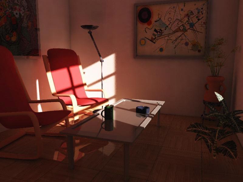
25 In practice Radiosity is computationally expensive, so rarely suitable for real-time rendering. However, it can be used in conjunction with light mapping.

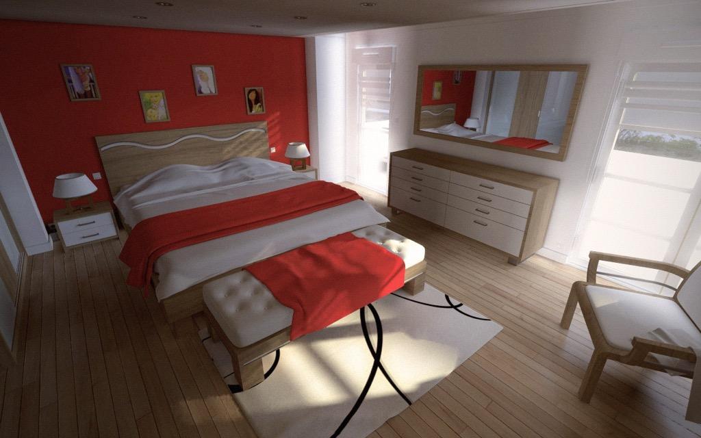
26 The payoff

27

28

29 Geometric light sources

30 Real-time Global Illumination v=pq39xb7odh8

31 Sources radiosity.htm gr_lectures.html HyperGraph/radiosity/overview_2.htm gpugems2_chapter39.html

32 COMP3421 B-Splines

33 Quick Recap: Curves We want a general purpose solution for drawing curved lines and surfaces. It should: Be easy and intuitive to draw curves Support a wide variety of shapes, including both standard circles, ellipses, etc and "freehand" curves. Be computationally cheap.

34 Bézier curves Have the general form: where m is the degree of the curve and P0...Pm are the control points.

35 Bernstein polynomials where: is the binomial function.

36 Bernstein polynomials For the most common case, m = 3:

37 Problems Local control - Moving one control point affects the entire curve. Incomplete - No circles, elipses, conic sections, etc.

38 Problem: Local control These curves suffer from non-local control. Moving one control point affects the entire curve. Each Bernstein polynomial is active (non-zero) over the entire interval [0,1]. The curve is a blend of these functions so every control point has an effect on the curve for all t from [0,1]

39 Splines A spline is a smooth piecewise-polynomial function (for some measurement of smoothness). The places where the polynomials join are called knots. A joined sequence of Bézier curves is an example of a spline.

40 Local control A spline provides local control. A control point only affects the curve within a limited neighbourhood.

41 Bézier splines We can draw longer curves as sequences of Bézier sections with common endpoints:

42 Parametric Continuity A curve is said to have C n continuity if the nth derivative is continuous for all t: C 0: the curve is connected. C 1: a point travelling along the curve doesn't have any instantaneous changes in velocity. C2: no instantaneous changes in acceleration

43 Geometric Continuity A curve is said to have G n continuity if the normalised derivative is continuous for all t. G 1 means tangents to the curve are continuous G 2 means the curve has continuous curvature.

44 Continuity Geometric continuity is important if we are drawing a curve. Parametric continuity is important if we are using a curve as a guide for motion.

45 Bézier splines If the control points are collinear, the the curve has G 1 continuity:

46 Drawing

47 Bézier splines If the control points are collinear and equally spaced, the curve has C 1 continuity:

48 Motion

49 B-splines We can generalise Bézier splines into a larger class called basis splines or B-splines. A B-spline of degree m has equation: where L is the number of control points, with

50 B-splines The function is defined recursively: (Note: this formulation differs slightly from the one in the textbook)

51 Knot vector The sequence is called the knot vector. The knots are ordered so Knots mark the limits of the influence of each control point. Control point Pk affects the curve between knots tk and tk+m+1.

52 Number of Knots The number of knots in the knot vector is always equal to the number of control points plus the order of the curve. E.g., a cubic (m=3) with five control points has 9 items in the knot vector. For example: (0,0.125,0.25,0.375,0.5,0.625,0.75,0.875,1)

53 Uniform / Non-uniform Uniform B-splines have equally spaced knots. Non-uniform B-splines allow knots to be positioned arbitrarily and even repeat. A multiple knot is a knot value that is repeated several times. Multiple knots create discontinuities in the derivatives.

54 Continuity A polynomial of degree m has C m continuity. A knot of multiplicity k reduces the continuity by k. So, a uniform B-spline of degree m has C m-1 continuity.

55 Interpolation A uniform B-spline approximates all of its control points. A common modification is to have knots of multiplicity m+1 at the beginning and end in order to interpolate the endpoints. This is called clamping.

56 Moving Controls and Knots Moving Controls: Adjacent control points on top of one another causes the curve to pass closer to that point. With m adjacent control points the curve passes through that point. Moving Knots: Across a normal knot the continuity for and degree curve is C m-1. Each extra knot with the same value reduces continuity at that value by one.

57 Quadratic and Cubic The most commonly used B-splines are quadratic (m=2) and cubic (m=3). Uniform quadratic splines have C 1 (and G 1 ) continuity. Uniform cubic splines have C 2 (and G 2 ) continuity.

58 Bezier and B-Spline A Bézier curve of degree m is a clamped uniform B-spline of degree m with L=m+1 control points. A Bézier spline of degree m is a sequence of bezier curves connected at knots of multiplicity m. A quadratic piecewise Bézier knot vector with 9 control points will look like this (0,0,0,0.25,0.25,0.5,0.5,0.75,0.75,1,1,1).

59 Incomplete Conic sections are the intersection between cones and planes.

60 Rational Bézier Curves We can create a greater variety of curve shapes if we weight the control points: A higher weight draws the curve closer to that point. This is called a rational Bézier curve.

61 Rational Bézier Curves Rational Bézier curves can exactly represent all conic sections (circles, ellipses, parabolas, hyperbolas). This is not possible with normal Bézier curves. If all weights are the same, it is the same as a Bezier curve

62 Rational B-splines We can also weight control points in B-splines to get rational B-splines:

63 NURBS Non-uniform rational B-splines are known as NURBS. NURBS provide a power yet efficient and designer-friendly class of curves.

64

65 Closed curves A unclamped uniform B-spline of degree m is a closed loop if the first m control points match the last m control points.

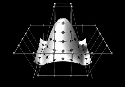
66 Surfaces

67 Surfaces We can create 2D surfaces by parameterising over two variables: Where is any particular spline function we choose (Bezier, B-spline, NURBS) and denote an LxM array of control points.

68 COMP3421 Colour Theory

69 What is colour? The experience of colour is complex, involving: Physics of light, Electromagnetic radiation Biology of the eye, Neuropsychology of the visual system.

70

71

72

73 Physics of light Light is an electromagnetic wave, the same as radio waves, microwaves, X-rays, etc. The visible spectrum (for humans) consists of waves with wavelength between 400 and 700 nanometers.

74 Non-spectral colours Some light sources, such as lasers, emit light of essentially a single wavelength or pure spectral light (red,violet and colors of the rainbow). Other colours (e.g. white, purple, pink,brown) are non-spectral. There is no single wavelength for these colours, rather they are mixtures of light of different wavelengths.

75 Colour perception The retina (back of the eye) has two different kinds of photoreceptor cells: rods and cones. Rods are good at handling low-level lighting (e.g. moonlight). They do not detect different colours and are poor at distinguishing detail. Cones respond better in brighter light levels. They are better at discerning detail and colour.

76 The Eye resources/second-look-series/materials

77 Tristimulus Theory Most people have three different kinds of cones which are sensitive to different wavelengths.

78 Colour blending As a result of this, different mixtures of light will appear to have the same colour, because they stimulate the cones in the same way. For example, a mixture of red and green light will appear to be yellow.

79 Colour blending We can take advantage of this in a computer by having monitors with only red, blue and green phosphors in pixels. Other colours are made by mixing these lights together.

80 Colour blending Can we make all colours this way? No. Some colours require a negative amount of one of the primaries (typically red).

81 Colour blending What does this mean? Algebraically, we write: to indicate that colour C is equivalent (appears the same as) r units of red, g units of green and b units of blue.

82 Colour blending A colour with wavelength 500nm (cyan/teal) has: We can rearrange this as: So if we add 0.3 units of red to colour C, it will look the same as the given combination of green and blue. Data source: C X 0.3 R 0.49 G X 0.11 B

83 Tristimulus Theory and Colour Blending applets/locus.html applets/colormatching.html

84 Complementary Colors Colours that add to give white (or at least grey) are called complementary colours eg red and cyan Retinal fatigue causes complementary colours to be seen in after-images light/complementary-colours.htm

85 Describing colour We can describe a colour in terms of its: Hue - the colour of the dominant wavelength such as red Luminance - the total power of the light (related to brightness) Saturation - the purity of the light i.e the percentage of the luminance given by the dominant hue (the more grey it is the more unsaturated)

86 Spectral Density Hue is the peak or dominant wavelength Luminance is related to the intensity or area under the entire spectrum Saturation is the percentage of intensity in the dominant area

87 Physics vs Perception We need to be careful with our language. Physical and perceptual descriptions of light differ. A red light and a blue light of the same physical intensity will not have the same perceived brightness (the red will appear brighter). Intensity, Power = physical properties Luminance, Brightness = perceptual properties

88 Describing colour Computer science offers a few poorer cousins to these perceptual spaces that may also turn up in your software interface, such as HSV and HLS. They are easy mathematical transformations of RGB, and they seem to be perceptual systems because they make use of the hue-lightness/value-saturation terminology. But take a close look; don t be fooled. Perceptual color dimensions are poorly scaled by the color specifications that are provided in these and some other systems. For example, saturation and lightness are confounded, so a saturation scale may also contain a wide range of lightnesses (for example, it may progress from white to green which is a combination of both lightness and saturation). Likewise, hue and lightness are confounded so, for example, a saturated yellow and saturated blue may be designated as the same lightness but have wide differences in perceived lightness. These flaws make the systems difficult to use to control the look of a color scheme in a systematic manner. If much tweaking is required to achieve the desired effect, the system offers little benefit over grappling with raw specifications in RGB or CMY.

89 Standardisation A problem with describing colours as RGB values is that depends on what wavelengths we define as red, green and blue. Different displays emit different frequencies, which means the same RGB value will result in slightly different colours. We need a standard that is independent of the particular display.

90 The CIE standard The CIE standard, also known as the XYZ model, is a way of describing colours as a three dimensional vector (x,y,z) with: X, Y and Z are called imaginary colours. It is impossible to create pure X, it is just a useful mathematical representation.

91 The CIE standard Spectral colours Non-spectral colours E = (1/3, 1/3, 1/3)

92 Gamut Any output device has a certain range of colours it can represent, which we call its gamut. We can depict this as an area on the CIE chart. If a monitor has red, green and blue phosphors then the gamut is the interior of the triangle joining those points.

93 RGB Gamut

94 RGB Gamut What is wrong with this picture?

95 Gamut mapping How do we map an (x, y, z) colour from outside the gamut to a colour we can display? We want to maintain: Approximately the same hue Relative saturation to other colours in the image.

96 Rendering intents There are four standard rendering intents which C describe approaches to gamut mapping. The definitions are informal. Implementations vary.

97 Absolute colormetric Map C to the nearest point within C C' the gamut. Distorts hues. Does not preserve relative saturation.

98 Relative colormetric Desaturate C until it lies in the gamut. C Maintains hues more C' closely. Does not preserve relative saturation.

99 Perceptual C1 C2 Desaturate all colours until they all lie in the gamut. C1' C2' Maintains hues. C3 C3' Preserves relative saturation. Removes a lot of saturation.

100 Saturation Attempt to maintain saturated colours. C1 C2 C2' There appears to be C1' no standard C3 algorithmic C3' implementation.

101 Demo applets/gamutmapping.html

102 Colour space Standard colour representations: RGB = Red, Green, Blue CMYK = Cyan, Magenta, Yellow, Black HSV = Hue, Saturation, Value (Brightness) HSL = Hue, Saturation, Lightness

103 RGB Colour is expressed as the addition of red, green and blue components. This is called additive colour mixing. It is the most common model for computer displays.

104 CMY CMY is a subtractive colour model, typically used in describing printed media. Cyan, magenta and yellow are the contrasting colours to red, green and blue respectively. I.e.: Cyan pigment/ink absorbs red light.

105 CMYK Real coloured inks do not absorb light perfectly, so darker colours are achieved by adding black ink to lower the overall brightness. The K in CMYK stands for "key" and refers to black ink.

106 HSV HSV (aka HSB) is an attempt to describe colours in terms that have more perceptual meaning (but see earlier proviso). H represents the hue as an angle from 0 (red) to 360 (red) S represents the saturation from 0 (grey) to 1 (full colour) V represents the value/brightness form 0 (black) to 1 (bright colour).

107 HSL HSL (aka HLS) replaces the brightness parameter with a (perhaps) more intuitive lightness value. H represents the hue as an angle from 0 (red) to 360 (red) S represents the saturation from 0 (grey) to 1 (full colour) L represents the lightness form 0 (black) to 1 (white).

108 Video v=z9sen1htu5o