Intensity Transformations and Spatial Filtering

Transcription

1 77 Chapter 3 Intensity Transformations and Spatial Filtering Spatial domain refers to the image plane itself, and image processing methods in this category are based on direct manipulation of pixels in an image. Two principal categories of spatial processing are intensity transformations and spatial filtering. Intensity transformations operate on single pixels of an image for the purpose of contrast manipulation and image thresholding. Spatial filtering deals with performing operations, such as image sharpening, by working in a neighbourhood of every pixel in an image. 3.1 Background The Basics of Intensity Transformations and Spatial Filtering Generally, spatial domain techniques are more efficient computationally and require less processing resources to implement. The spatial domain processes can be denoted by the expression g( x, y) = T[ f ( x, y)] (3.1-1) where f(x, y) is the input image, g(x, y) is the output image, and T is an operator on f defined over a neighbourhood of point (x, y). The operator can apply to a single image or to a set of images.

2 78 Typically, the neighbourhood is rectangular, centered on (x, y), and much smaller than the image. Example: Suppose that the neighbourhood is a square of size 3 3 and the operator T is defined as compute the average intensity of the neighbourhood. At an arbitrary location in an image, say (10, 15), the output g(10, 15) is computed as the sum of f(10, 15) and its 8-neighbourhood is divided by 9. The origin of the neighbourhood is then moved to the next location and the procedure is repeated to generate the next value of the output image g.

3 The smallest possible neighbourhood is of size 1 1. Example: 79

4 3.2 Some Basic Intensity Transformation Functions 80 Intensity transformations are among the simplest of all image processing techniques. We use the following expression to indicate a transformation s = T( r) where T is a transformation that maps a pixel value r into a pixel value s. Image Negatives The negative of an image with intensity levels in the range [0, L 1] is obtained by using the negative transformation shown in Figure 3.3, which is given by s = L 1 r (3.2-1)

5 Example: 81 The negative transformation can be used to enhance white or gray detail embedded in dark regions of an image. Log Transformations The general form of the log transformations is s = clog(1 + r) (3.2-2) where c is a constant, and r 0. The log transformation maps a narrow range of low intensity values in the input into a wider range of output levels. We use the transformation of this type to expend the values of dark pixels in an image while compress the higher-level values. The opposite is true of the inverse log transformation.

6 82 Example: Figure 3.5(a) shows a Fourier spectrum with values in the range 6 0 to Figure 3.5(b) shows the result of applying (3.2-2) to the spectrum values, which will rescale the values to a range of 0 to 6.2, and displaying the results with an 8-bit system. Power-Law (Gamma) Transformations Power-law transformations have the basic form s = cr γ (3.2-3) where c and γ are positive constants. A variety of devices used for image capture, printing, and display according to a power-law. By convention, the exponent in the power-law equation is referred to as gamma.

7 83 Unlike the log function, changing the value of γ will obtain a family of possible transformations. As shown in Figure 3.6, the curves generated with values of γ > 1 have exactly the opposite effect as those generated with values of γ < 1. The process used to correct these power-law response phenomena is called gamma correction.

8 Example: 84 Gamma correction is important if displaying an image accurately on a computer screen is of concern. Gamma correction has become increasingly important as the use of digital images over the Internet has increased. In addition to gamma correction, power-law transformations are very useful for general-purpose contrast manipulation.

9 85 Example 3.1: Contrast enhancement using power-law transformations.

10 86 Example 3.2: Another illustration of power-law transformations. Figure 3.9(a) shows the opposite problem of Figure 3.8(a).

11 Piecewise-Linear Transformation Functions 87 A complementary approach to the abovementioned methods is to use piecewise linear functions. Contrast stretching One of the simplest piecewise linear functions is a contraststretching transformation. Contrast-stretching transformation is a process that expands the range of intensity levels in an image so that it spans the full intensity range of the recording medium or display device. Example:

12 Intensity-level slicing 88 Highlighting a specific range of intensities in an image often is of interest. The process, often called intensity-level slicing, can be implemented in several ways, though basic themes are mostly used. One approach is to display in one value all the values in the range of interest and in another all other intensities, as shown in Figure 3.11 (a). Another approach is based on the transformation in Figure 3.11(b), which brightens (or darkens) the desired range of intensities but leaves all other intensities levels in the image unchanged.

13 Example 3.3: Intensity-level slicing 89 Figure 3.12 (b) shows the result of using a transformation of the form in Figure 3.11 (a), with the selected band near the top of the scale, because the range of interest is brighter than the background. Figure 3.12 (c) shows the result of using the transformation in Figure 3.11 (b) in which a band of intensities in the mid-gray region around the mean intensity was set to black, while all other intensities were unchanged.

14 Bit-plane slicing 90 Instead of highlighting intensity-level ranges, we could highlight the contribution made to total image appearance by specific bits. Figure 3.13 shows an 8-bit image, which can be considered as being composed of eight 1-bit planes, with plane 1 containing the lowest-order bit of all pixels in the image and plane 8 all the highest-order bits. Example:

15 91 Note that each bit plane is a binary image. For example, all pixels in the border have values , which is the binary representation of decimal 194. Those values can be viewed in Figure 3.14 (b) through (i). Decomposing an image into its bit planes is useful for analyzing the relative importance of each bit in the image. Example:

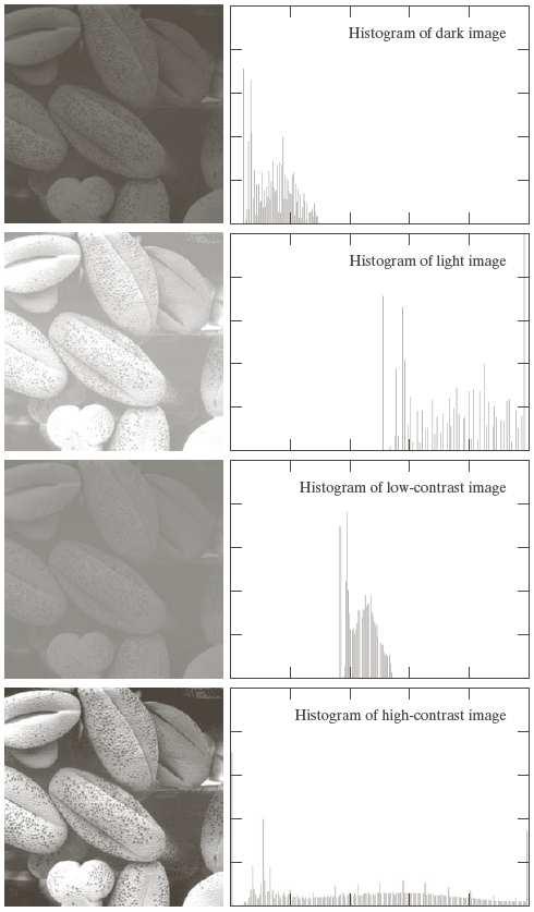
16 3.3 Histogram Processing 92 The histogram of a digital image with intensity levels in the range [0, L 1] is a discrete function h( rk ) = nk, where r k is the kth intensity value and n k is the number of pixels in the image with intensity r k. It is common practice to normalize a histogram by diving each of its components by the total number of pixels in the image, denoted by MN, where M and N are the row and column dimensions of the image. A normalized histogram is given by nk p( rk ) =, for k = 0,1,2,..., L 1. MN p( r k ) can be seen as an estimate of the probability of occurrence of intensity level r k in an image. The sum of all components of a normalized histogram is equal to 1. Histograms are the basic for numerous spatial domain processing techniques. Example: Figure 3.16, which is the pollen image of Figure 3.10 shown in four basic intensity characteristics: dark, light, low contrast, and high contrast, shows the histograms corresponding to these image. The vertical axis corresponds to value of h( rk ) = nk or p( r ) = n / MN if the values are normalized. k k

17 93

18 Histogram Equalization 94 We consider the continuous intensity values and let the variable r denote the intensities of an image. We assume that r is in the range [0, L 1]. We focus on transformations (intensity mappings) of the form s = T( r) 0 r L 1 (3.3-1) that produce an output intensity level s for every pixel in the input image having intensity r. Assume that (a) T( r ) is a monotonically increasing function in the interval 0 r L 1, and (b) 0 T( r) L 1 for 0 r L 1. In some formations to be discussed later, we use the inverse r = T 1 ( s) 0 s L 1 (3.3-2) in which case we change condition (a) to (a ') T( r ) is a strictly monotonically increasing function in the interval 0 r L 1. Figure 3.17 (a) shows a function that satisfies conditions (a) and (b).

19 95 From Figure 3.17 (a), we can see that it is possible for multiple values to map to a single value and still satisfy these two conditions, (a) and (b). That is, a monotonic transformation function can perform a one-to-one or many-to-one mapping, which is perfectly fine when mapping from r to s. However, there will be a problem if we want to recover the values of r uniquely from the mapped values. As Figure 3.17 (b) shows, requiring that T( r ) be strictly monotonic guarantees that the inverse mappings will be single valued. This is a theoretical requirement that allows us to derive some important histogram processing techniques. The intensity levels in an image may be viewed as random variables in the interval [0, L 1]. A fundamental descriptor of a random variable is its probability density function (PDF). Let pr ( r) and ps ( s ) denote the probability density functions of r and s. A fundamental result from basic probability theory is that if pr ( r ) and T( r ) are known, and T( r ) is continuous and differentiable over the range of values of interest, then the PDF of the transformed variable s can be obtained using the formula

20 dr ps( s) = pr (r) ds (3.3-3) 96 A transformation function of particular importance in image processing has the form r s = T(r) = ( L 1) pr ( ω) dω (3.3-4) where ω is a dummy variable of integration. 0 The right side of (3.3-4) is recognized as the cumulative distribution function of random variable r. Since PDFs always are positive, the transformation function of (3.3-4) satisfies condition (a) because the area under the function cannot decreases as r increases. When the upper limit in (3.3-4) is r = ( L 1), the integral evaluates to 1 (the area under a PDF curve always is 1), so the maximum value of s is ( L 1) and condition (b) satisfies as well. Using (3.3-3) and recalling the Leibniz s rule that saying the derivative of a definite integral with respect to its upper limit is the integrand evaluated at the limit, we have ds dt ( r) = dr dr d = ( L 1) p ( ) d dr = ( L 1) p ( r) r r 0 r ω ω (3.3-5) Substituting this result for dr / ds in (3.3-3), yields

21 dr ps( s) = pr ( r) ds 97 1 = pr ( r) ( L 1) p ( r ) 1 = 0 s L 1 L 1 r (3.3-6) which shows the that ps( s ) always is uniform, independently of the form of pr ( r ). Example 3.4: Illustration of (3.3-4) and (3.3.6) Suppose that the continuous intensity values in an image have the PDF pr ( r) = 0 2r ( L 1) 2 for 0 r L 1 otherw ise

22 From (3.3-4), 98 r s = T( r) = ( L 1) pr ( ω) dω (3.3-4) r 2 2 r = ωdω = ( L 1) L Consider an image in which L = 10, and suppose that a pixel at ( x, y ) in the input image has intensity r = 3. Then, the pixel at 2 ( x, y ) in the new image is s = T( r) = r / 9 = 1. We can versify that the PDF of the intensities in the new image is uniform by substituting pr ( r ) into (3.3-6) and using the facts that s = r 2 / ( L 1), r is nonnegative, and L > 1: dr ps( s) = pr ( r) ds (3.3-6) 2r = ( L 1) 2 ds dr 1 2 2r d r = 2 ( L 1) dr L r ( L 1) 1 = = 2 ( L 1) 2r L 1

23 99 For discrete values, we deal with probabilities (histogram values) and summations instead of probability density functions and integrals. The probability of occurrence of intensity level r k in a digital image is approximated by nk pr ( rk ) = k = 0,1,2,..., L 1 (3.3-7) MN where MN is the total number of pixels in the image, n k is the number of pixels having intensity r k, and L is the number of possible intensity levels in the image. The discrete form of the transformation in is r s = T( r) = ( L 1) pr ( ω) dω (3.3-4) s = T( r ) = ( L 1) p ( r ) k k r j j= 0 j= 0 0 k k ( L 1) = n j k = 0,1,2,..., L 1 MN (3.3-8) The transformation (mapping) ( ) k T r in (3.3-8) is called a histogram equalization transformation.

24 100 Example 3.5: A simple illustration of history equalization. Suppose that a 3-bit image ( L = 8) of size pixels ( MN = 4096 ) has the intensity distribution shown in Table 3.1. The histogram of our hypothetical image is sketched in Figure 3.19 (a). By using (3.3-8), we can obtain values of the histogram equalization function: 0 s = T( r ) = 7 p ( r ) = 7 p ( r ) = 1.33, 0 0 r j r 0 j= 0

25 101 1 s = T( r ) = 7 p ( r ) = 7 p ( r ) + 7 p ( r ) = 3.08, 1 1 r j r 0 r 1 j= 0 s 2 = 4.55, s 3 = 5.67, s 4 = 6.23, s 5 = 6.65, s 6 = 6.86 s 7 = This function is shown in Figure 3.19 (b). Then, we round them to the nearest integers: , and s = s = s = s = s = s = s = s = which are the values of the equalized histogram. Observe that there are only five distinct levels: s0 1 : 790 pixels s1 3 : 1023 pixels s2 5 : 850 pixels s3 6 : 985 ( ) pixels s5 7 : 448 ( ) pixels Total: 4096 Dividing these numbers by MN = 4096 would yield the equalized histogram shown in Figure 3.19 (c). Since a histogram is an approximation to probability density function, and no new allowed intensity levels are created in the process, perfectly flat histograms are rare in practical applications of histogram equalization. Therefore, in general, it cannot be proved that discrete histogram equalization results in a uniform histogram.

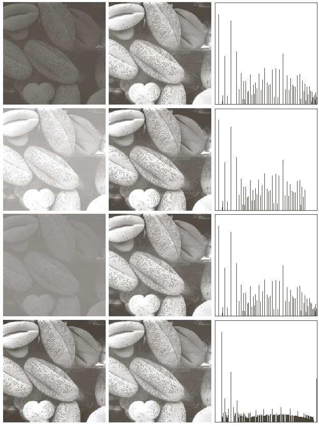
26 102 Given an image, the process of histogram equalization consists simply of implementing s k ( L 1) k = n j MN, (3.3-8) j = 0 which is based on information that can be extracted directly from the given image, without the need for further parameter specifications. The inverse transformation from s back to r is denoted by r = T 1 ( s ) k = 0,1,2,..., L 1 (3.3-9) k k Although the inverse transformation is not used in the histogram equalization, it plays a central role in the histogram-matching scheme. Example 3.6: Histogram equalization The left column in Figure 3.20 shows the four images from Figure The center column in Figure 3.20 shows the result of performing histogram equalization on each of the images in left. The histogram equalization did not have much effect on the fourth image because the intensities of this image already span the full intensity scale.

27 103

28 104 Figure 3.21 shows the transformation functions used to generate the equalized images in Figure 3.20.