3 Dimensional modeling of shelf margin clinoforms of the southwest Karoo Basin, South Africa.

Transcription

1 3 Dimensional modeling of shelf margin clinoforms of the southwest Karoo Basin, South Africa. Joshua F Dixon A. Introduction The Karoo Basin of South Africa contains some of the best exposed shelf margin strata in the world. These strata outcrop as sandy deltaic wedges interbedded with fine grained material. Little detailed work has been carried out in the shelf edge successions in this area and as such, correlation of the different stratigraphic levels throughout the region remains problematic. Due to the arid climate in the southwest Karoo, the area has little vegetation and a thin soil cover. This contributes to a characteristic erosional profile in which the erosion resistant deltaic sand wedges form cliffs capped by plateaus whereas areas of fine grained material are characterized by low gradient slopes. The objective of this project is to map 2 of these these sandy wedges (stratigraphic horizon 1 and 2 ) throughout the region. The maps generated will be useful for 1) aiding in the correlation of sand bodies between different mountains, 2) identifying areas with outcrop and, 3) determining clinoform gradient. B. Dataset 1. Requirements As a large component of this project will involve spatial analysis of elevation data, a detailed digital elevation model (DEM) will be required. This elevation data will be supplemented with point data collected with a handheld global positioning system (GPS) device in Spring 2009 and available topographic maps. 2. Data Acquisition The highest resolution DEM data available in a non US region such as South Africa is acquired using the Advanced Spaceborne Thermal Emission and Reflection Radiometer (ASTER) instrument. Two ASTER 0.85x0.85decimal degree raster datasets were downloaded from bin/api/ims.cgi?mode=mainsrch&js=1 centered around the area of interest at approximately ( 32 50, ). Four 1:50,000 topographic map rasters were downloaded from East View Cartographic centered on the area of interest. A waypoint dataset was collected in the field in Spring Each point was collected whilst walking out specific sand bodies. These data were collected relative to the WGS 84 datum in decimal degrees with a Garmin etrex VISTA unit. C. Data Conversion All data must be converted to the UTM coordinate with the following properties. Property Value Spatial Reference WGS_1984_UTM_Zone34S Linear Unit Meter ( ) 1

2 Angular Unit Degree ( ) False Easting False Northing Central Meridian 21 Scale Factor Latitude of Origin 0 Datum D_WGS_1984 D. Data Processing The goal of this project is to ultimately produce maps of the cliffs which define sandstone outcrops, as such; this is an exercise of identification and correlation of cliffs which are fundamentally areas of high gradient. The cliffs are not clearly expressed in either the topographic maps or unprocessed DEM data. This is illustrated in the figures below. Stratigraphic Unit 2 Clearly recognizable cliff, c.15m high. In Stratigraphic Unit 1 (above) Aerial photograph facing north east (courtesy, Asle Strøm) 2

3 Approximate field of view of aerial photograph. No clear indication of cliff in topomap Topographic map of same area, approximate location of cliff highlighted. 3

4 No clear indication of cliff in DEM DEM of same area, approximate area of cliff highlighted. To identify the cliffs, the DEM data must be processed 1. Initially the gradient was extracted from the DEM data (ArcToolbox/Spatial Analyst Tools/Surface/Slope). A new slope raster was created from both original rasters. Output measurement=degree, Z factor=1. The area highlighted in the figures above is now shown below featuring the new slope rasters. 4

5 Slope map of the same area shown above. Light green represents low gradients, dark blue represents high gradient. The cliff top is thus the contact between light green (low gradient areas) and dark blue (high gradients). 2. A second method was also tried using the curvature tool (ArcToolbox/Spatial Analyst Tools/Surface/curvature). This function extracts the second derivative of the surface (slope of the slope), returning negative values for the convex up rollover at the top of a cliff and a negative value for the concave up curvature at the base of a cliff. The maps generated were not used any further as they contained low signal to noise ratios and as such did not produce laterally correlative values associated with cliff locations. E. Additional Controls on Picking of Surfaces The slope maps generated do not yield maps with laterally continuous (correlatable) bands of high surface gradient. Several scenarios which cause this lateral discontinuity include: i. The case in which 2 cliffs formed by 2 sand wedges converge such that one is stacked above the other to form 1 cliff ii. Cases in which a cliff or series of cliffs are buried by a landslide iii. Finally, the most common, areas in which the cliffs are below the vertical resolution of the data or are simply so low relief that the gradient recorded in these low resolution data is indistinguishable from flat land 5

6 Because of this, other control points will be required push the correlations into areas of poor data, and to complete correlations between areas of good quality data. 1. The first additional data source is the GPS dataset collected in the field. These waypoint data were collected whilst walking out the two stratigraphic levels of interest. With spacing below 100m in most cases these will serve as a accurate constraint when correlating the cliffs. The problem with the GPS point data is that they were only collected on one mountain within the region. As such, other constraints will be needed to expand the correlations to adjacent mountains. 2. A second constraint on cliff location can be generated remotely from the DEM data in ArcMap. Using 3D Analyst, lines were interpolated and profile graphs were generated. The lines were positioned at various locations on various mountains within the area of interest. Lines were drawn from summits to the valleys below (see map below). These were then exported to Excel where the different cliffs could be identified by comparing the elevation of slope breaks in different profiles beginning with profiles which were within the area with GPS datapoint coverage. The elevations of these slope breaks and their position along the profile was then noted. These elevation points along the profiles would act as inferred data points on the stratigraphic horizons. Mountain Side Elevation Profiles, Southwest Karoo Basin, South Africa Elevation (m) Distance along profile (m) *2 1 *3 1 *4 1 *2 7 *6 5 *3 5 *10 9 *8 9 *8 5 *8 15 *13 15 *14 15 *20 19 *16 19 *18 17 Elevation profiles for 16 transects in the area of interest. Each transect is labeled with reference to its start and end points. See map below for location data of these points. Highlighted on this figure are the cliffs corresponding to the 2 stratigraphic levels (sand wedges 1 and 2 ). 6

7 Topographic map with DEM and end points for topographic profiles overlain. F. Picking Stratigraphic Horizons n the X Y Plane Now that we have an increased data point control for the position (in x,y and z coordinates) we can correlate the horizons between these known and inferred points using the slope maps created in a previous step. One potential cause of error is the correlation of two areas of high gradient which are close together in the x y plane but correspond to separate cliffs vertically. this problem is illustrated below; 7

8 a b The figure above is a slope map within the area of interest. Highlighted are 2 possible correlations of the high gradient areas (cliffs). Correlation in this area is problematic as several high gradient areas converge and split producing several possible interpretations. As gradient does not indicate slope direction, it is not possible to distinguish an isolated high circled by cliffs (interpretation a) or an isolated low circled by cliffs (alternate explanation for a) from a terrace or ledge that defines a stepped profile (interpretation b). 1. The following method was devised to remove this potential error i. Reclassify the slope raster to give values of 1 for areas with gradient (defined as areas with slope greater than 6 ) and values of 0 for areas with gradient less than 6. ii. The raster calculator was then used to multiply the reclassified raster from step 1 by the DEM raster. iii. The calculation output is now essentially a DEM clipped to areas with significant slope (see below). 8

9 Horizon 1 Horizon 2 Now we can see plateaus (or terraces/steps) that are bound by high gradient areas. Because the map shows elevation, we can differentiate slopes dipping in different directions, and also sloped areas at different elevations. This figure confirms that example b on the previous page was the correct example. 2. Now that we have removed this potential source of error, we can begin the correlation of the stratigraphic horizons of interest. i. First, 2 new shapefiles (feature type: polyline) were created in ArcCatalog. These will be used for the 2 respective stratigraphic levels of interest; 1 and 2. ii. Lines were plotted in the x y plane using the GPS waypoints, points derived from the topographic profiles and finally, the clipped DEM data as constraints. These lines were not continuous across the field area. The mapped lines are presented below. 9

10 Topographic map with traced stratigraphic horizon outcrop lines highlighted (red=1, blue=2). It is clear that the correlation was carried out with greater confidence within the area of GPS data coverage (highlighted by green polygon). G. Conversion of Correlated lines. The ultimate aim of this project is to produce maps of the 2 stratigraphic surface by 10

11 interpolating the elevation of the horizons between areas of outcrop. To do this, the line shapefiles must be converted so that the data can be manipulated. 1. The line vertices were converted to point files using ArcToolbox/Data Management Tools/Features/Feature vertices to points. This provides us with point location data which are much easier to manipulate to produce maps. 2. These point data however do not have elevation information. This problem was overcome using the tool: ArcToolbox/Spatial Analyst Tools/Extraction/Extract values to points. The elevation values from the DEM were extracted to each point datum adding an extra field to the attribute table (elevation). H. Contouring the Data. Several spatial interpolation techniques are available in ArcMap, for this project Natural Neighbor (ArcToolbox/Spatial Analyst Tools/Interpolation/Natural Neighbor) was chosen to interpolate the point data to creat elevation maps. This method was chosen as it does not produce peaks or pits not present in the data. Other attempts using various kriging, inverse distance weighting and spline produced stratigraphically unlikely outputs and were not explored further. The raster outputs of the interpolation were limited by the spacing of the data points such that the maps for each level had slightly different aerial extents. These are presented below. 11

12 Interpolated elevation map of stratigraphic horizon 1 with contol points overlain. 12

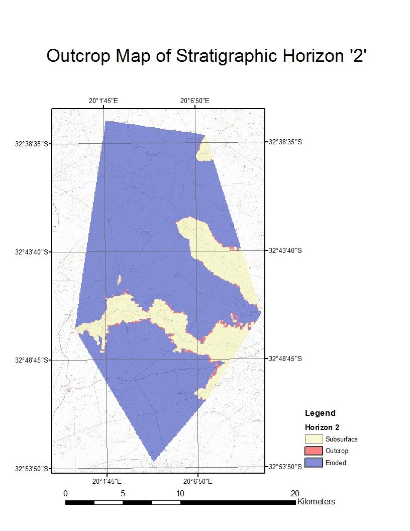
13 Interpolated elevation map of stratigraphic horizon 2 with contol points overlain. I. Final Manipulation of the Data. The maps generated in the previous step can now be manipulated to deliver the maps and information outlined at the outset of the project. The required maps incude: i. Isopach (thickness) maps between surfaces 1 and 2 ii. Predicted outcrop location maps for surfaces 1 and 2 iii. Gradient map of surface 1 1. Isopach map The creation of the isopach map was a simple process of using the raster calculater to subtract surface 1 from surface 2. The output was limited to areas with data coverage of both surfaces. This was not a big problem as the control points were positioned such that both maps would have a similar aerial extent. See appendix for map. 13

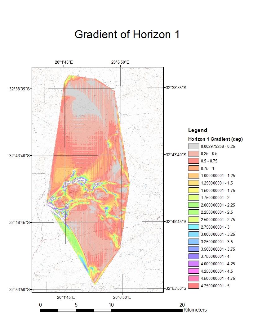
14 2. Predicted outcrop location map 2 maps were generated by subtracting the DEM raster from the elevation rasters of surface 1 and 2 respectively. This yields maps in the values represent the inferred vertical distance between the horizon and the earths surface. Positive values represent areas where the horizon has been eroded (above the earths surface) and negative values represent areas where the horizon is in the subsurface. These values were reclassified into 3 bins ( 1000 to 2; 2 to +2; +2 to +1000) these bins represent areas where the horizon is below the surface, near to surface or outcropping and above the surface respectively. Values of ±2 were added to the outcrop bin to account for the potential innacuracies in the interpolated values. See Appendix for map. 3. Gradient Map of Surface 1 This map was generated simply by applying the slope function (ArcToolbox/Spatial Analyst Tools/Surface/Slope) to the isopach map. This produces a map with the gradient of horizon 1 assuming that 2 was originally flat. See appendix for map. F. Appendix Notes on Maps Isopach Map of 2 1 Stratigraphic Interval This map shows a general thickening to the east with 2 anomalies. 1) at around E S (area of no color), thickness values are negative (interpolated surface one is above surface 2) this is disregarded as this is stratigraphically impossible and is a product of the interpolation process of surface 1 in an area with no data point control. 2)the area at the southwestern margin of data coverage reports values anomalously high given the regional thickening trend to the east. This is also attributed to lack of datapoint control at both surfaces in this area. Gradient of Horizon 1 This map contains a large amount of noise, most of which is attributed to local differences in elevation between closely spaced datapoints. For this reason, anomolously large gradients are mapped in areas of close datapoint coverage. The typical gradient of this surface relative to surface 2 is between 0.25 and 0.75 degrees, dipping to the north east. 14

15 15

16 16

17 17

18 18