Computer Vision II Lecture 4

Transcription

1 Computer Vision II Lecture 4 Color based Tracking Bastian Leibe RWTH Aachen leibe@vision.rwth-aachen.de

2 Course Outline Single-Object Tracking Background modeling Template based tracking Color based tracking Contour based tracking Tracking by online classification Tracking-by-detection Bayesian Filtering Multi-Object Tracking Articulated Tracking 2 Image source: Robert Collins

3 Recap: Estimating Optical Flow I(x,y,t 1) I(x,y,t) Optical Flow Given two subsequent frames, estimate the apparent motion field u(x,y) and v(x,y) between them. Key assumptions Brightness constancy: projection of the same point looks the same in every frame. Small motion: points do not move very far. Spatial coherence: points move like their neighbors. Slide credit: Svetlana Lazebnik 3

4 Recap: Lucas-Kanade Optical Flow Use all pixels in a K K window to get more equations. Least squares problem: Minimum least squares solution given by solution of Recall the Harris detector! Slide adapted from Svetlana Lazebnik 4

5 Recap: Iterative Refinement Estimate velocity at each pixel using one iteration of LK estimation. Warp one image toward the other using the estimated flow field. Refine estimate by repeating the process. estimate update estimate update x 0 x 0 Initial guess: Estimate: x Initial guess: Estimate: x Initial guess: estimate update Estimate: Iterative procedure Results in subpixel accurate localization. x 0 x Converges for small displacements. Slide adapted from Steve Seitz x 0 x 5

6 Recap: Coarse-to-fine Optical Flow Estimation u=1.25 pixels u=2.5 pixels u=5 pixels Image 1 u=10 pixels Image 2 Gaussian pyramid of image 1 Gaussian pyramid of image 2 Slide credit: Steve Seitz 6

7 Recap: Coarse-to-fine Optical Flow Estimation Run iterative LK Run iterative LK Warp & upsample... Image 1 Image 2 Gaussian pyramid of image 1 Gaussian pyramid of image 2 Slide credit: Steve Seitz 7

8 Recap: Shi-Tomasi Feature Tracker ( KLT) Idea Find good features using eigenvalues of second-moment matrix Key idea: good features to track are the ones that can be tracked reliably. Frame-to-frame tracking Track with LK and a pure translation motion model. More robust for small displacements, can be estimated from smaller neighborhoods (e.g., 5 5 pixels). Checking consistency of tracks Affine registration to the first observed feature instance. Affine model is more accurate for larger displacements. Comparing to the first frame helps to minimize drift. Slide credit: Svetlana Lazebnik J. Shi and C. Tomasi. Good Features to Track. CVPR

9 Recap: General LK Image Registration Goal Find the warping parameters p that minimize the sum-ofsquares intensity difference between the template image T(x) and the warped input image I(W(x;p)). LK formulation Formulate this as an optimization problem arg min p X 2 I(W(x; p)) T(x) x We assume that an initial estimate of p is known and iteratively solve for increments to the parameters p: arg min p X 2 I(W(x; p + p)) T(x) x 9

10 Recap: Step-by-Step Derivation Key to the derivation Taylor expansion around p I(W(x; p + p)) ¼ I(W(x; p)) p+o( p2 ) = I(W([x; y]; p 1 ; : : : ; p n )) i : : n : : n p 1 5 p p n to solve for Gradient Jacobian Increment parameters Slide credit: Robert Collins 10

11 Recap: LK Algorithm Iterate Warp I to obtain I(W([x, y]; p)) Compute the error image T([x, y]) I(W([x, y]; p)) Warp the gradient ri with W([x, y]; p) Evaluate at ([x, y]; p) (Jacobian) Compute steepest descent images Compute Hessian matrix Compute Compute P x p = H 1 P x Update the parameters p à p + p H = P h i T h i @p h i T T([x; y]) I(W([x; y]; p)) @p Until p magnitude is negligible 11 i T T([x; y]) I(W([x; y]; p)) [S. Baker, I. Matthews, IJCV 04]

12 12 [S. Baker, I. Matthews, IJCV 04] Recap: LK Algorithm Visualization

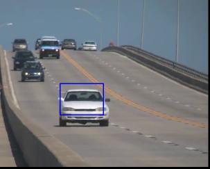
13 Example of a More Complex Warping Function Encode geometric constraints into region tracking Constrained homography transformation model Translation parallel to the ground plane Rotation around the ground plane normal W(x) = W obj P W t W α Q x Input for high-level tracker with car steering model. 13 [E. Horbert, D. Mitzel,, DAGM 10]

14 Today: Color based Tracking 14 Image source: Robert Collins

15 Topics of This Lecture Mean-Shift Mean-shift mode estimation Using mean-shift on color images Mean-Shift with Explicit Weight Images Histogram backprojection CAMshift approach Mean-Shift with Implicit Weight Images Comaniciu s approach Bhattacharyya distance Gradient ascent Comparison Qualitative intuition 15

16 Mean-Shift Mean-Shift Tracking Efficient approach to tracking objects whose appearance is defined by color. Actually, the approach is not limited to color. Can also use texture, motion, etc. Popular use for object tracking Very simple to implement Non-parametric method, does not make strong assumptions about the shape of the distribution Suitable for non-static distributions (as typical in tracking) Can be combined with dynamic models (Kalman filters, etc.) Good performance in practice 16

17 Mean-Shift: Intuitive Description Region of interest Center of mass Mean Shift vector Slide by Y. Ukrainitz & B. Sarel Objective: Find the densest region

18 Mean-Shift: Intuitive Description Region of interest Center of mass Mean Shift vector Slide by Y. Ukrainitz & B. Sarel Objective: Find the densest region

19 Mean-Shift: Intuitive Description Region of interest Center of mass Mean Shift vector Slide by Y. Ukrainitz & B. Sarel Objective: Find the densest region

20 Mean-Shift: Intuitive Description Region of interest Center of mass Mean Shift vector Slide by Y. Ukrainitz & B. Sarel Objective: Find the densest region

21 Mean-Shift: Intuitive Description Region of interest Center of mass Mean Shift vector Slide by Y. Ukrainitz & B. Sarel Objective: Find the densest region

22 Mean-Shift: Intuitive Description Region of interest Center of mass Mean Shift vector Slide by Y. Ukrainitz & B. Sarel Objective: Find the densest region

23 Mean-Shift: Intuitive Description Region of interest Center of mass Slide by Y. Ukrainitz & B. Sarel Objective: Find the densest region

24 Using Mean-Shift on Color Models Two main approaches 1. Explicit weight images Create a color likelihood image, with pixels weighted by the similarity to the desired color (best for unicolored objects). Use mean-shift to find spatial modes of the likelihood. 2. Implicit weight images Represent color distribution by a histogram. Use mean-shift to find the region that has the most similar color distribution. Slide credit: Robert Collins 24

25 Topics of This Lecture Mean-Shift Mean-shift mode estimation Using mean-shift on color images Mean-Shift with Explicit Weight Images Histogram backprojection CAMshift approach Mean-Shift with Implicit Weight Images Comaniciu s approach Bhattacharyya distance Gradient ascent Comparison Qualitative intuition 25

26 Mean-Shift on Weight Images Ideal case Want an indicator function that returns 1 for pixels on the tracked object and 0 for all other pixels. Instead Compute likelihood maps Value at a pixel is proportional to the likelihood that the pixel comes from the tracked object. Likelihood can be based on Color Texture Shape (boundary) Predicted location Slide credit: Robert Collins 26

27 Mean-Shift Tracking Idea Let pixels form a uniform grid of data points. Each pixel has a weight proportional to the likelihood that the pixel is on the object we want to track. Perform standard mean-shift using the weighted set of points. Slide credit: Robert Collins 27 Image source: Robert Collins

28 Mean-Shift Tracking A closer look at the procedure... Kernel weight evaluated at offset (a x) Weight from the likelihood image at pixel a Offset of pixel a to kernel center x Sum over all pixels a under kernel K Normalization term Mean-shift computes the weighted mean of all shifts (offsets), weighted by the likelihood under the kernel function. 28

29 Duality Property Duality Running mean-shift with kernel K on weight image w is equivalent to performing gradient ascent in a (virtual) image formed by convolving w by some shadow kernel H. Note: mode we are looking for is mode of location (x,y) likelihood, NOT mode of color distribution. Slide credit: Robert Collins 29 Image source: Robert Collins

30 Example: Face Tracking using Mean-Shift G. Bradski, Computer Vision Face Tracking for use in a Perceptual User Interface, IEEE Workshop On Applications of Computer Vision, Princeton, NJ, 1998, pp Slide credit: Robert Collins 30 Image source: Gary Bradski

31 Explicit Weight Images Histogram backprojection Histogram is an empirical estimate of p(color object) = p(c o) Bayes rule says: Simplistic approximation: assume p(o)/p(c) is constant. Use histogram h as a lookup table to set pixel values in the weight image. If pixel maps to histogram bucket i, set weight for pixel to h(i). Slide credit: Robert Collins 31 Image source: Gary Bradski

32 Side Note: Color Histograms for Recognition Using color histograms for recognition Works surprisingly well In the first paper (1991), 66 objects could be recognized almost without errors 32 [Swain & Ballard, 1991]

33 Localization by Histogram Backprojection Where in the image are the colors we re looking for? Query: object with histogram M Given: image with histogram I Compute the ratio histogram : R reveals how important an object color is, relative to the current image. Color is frequent on the object large M i Color is frequent in the image large I i This value is projected back into the image (i.e. the image values are replaced by the values of R that they index). The result image is convolved with a circular mask the size of the target object. Peaks in the convolved image indicate detected objects. Does this sound familiar? 33

34 Object Localization Results Example result after backprojection Looking for blue pullover 34 [Swain & Ballard, 1991]

35 Bradski s CAMshift Idea Find x,y location of mode by mean-shift. Determine z, roll angle µ by fitting an ellipse to the mode found using mean-shift. Slide credit: Robert Collins 35 Image source: Gary Bradski

36 36 Image source: Visualization: Bradski s CAMshift in Action

37 Problem: Scale Changes Window always has the same size When the object size changes, does not fit anymore Tracking soon diverges... Image source: 37

38 38 Image source: Visualization: Scale Adaptation in CAMshift

39 CAMShift Results Face tracking Using a skin color model in HSV color space 39 Video source: Gary Bradski

40 Applications: Perceptual User Interfaces Head tracking as input modality Controlling a flight simulator by head gestures 40 Video source: Gary Bradski

41 Topics of This Lecture Mean-Shift Mean-shift mode estimation Using mean-shift on color images Mean-Shift with Explicit Weight Images Histogram backprojection CAMshift approach Mean-Shift with Implicit Weight Images Comaniciu s approach Bhattacharyya distance Gradient ascent Comparison Qualitative intuition 41

42 Using Mean-Shift on Color Models Two main approaches 1. Explicit weight images Create a color likelihood image, with pixels weighted by the similarity to the desired color (best for unicolored objects). Use mean-shift to find spatial modes of the likelihood. 2. Implicit weight images Represent color distribution by a histogram. Use mean-shift to find the region that has the most similar color distribution. Slide credit: Robert Collins 42

43 Implicit Weight Images Sometimes the weight is not explicitly created Example: Mean-shift Tracking by Comaniciu et al. Weight is embedded into the matching procedure Comes out as a side effect of matching two pdfs. Interesting consequence Implicit weight image changes between iterations of mean-shift, as compared to iterating to convergence on an explicit weight image! We ll take a look at their approach and see how this works. D. Comaniciu, V. Ramesh, P. Meer. Kernel-Based Object Tracking, PAMI, Vol. 25(5), pp , Slide credit: Robert Collins 43

44 Mean-Shift Object Tracking Main idea: Match the pdf of the target object Slide by Y. Ukrainitz & B. Sarel 44

45 Mean-Shift Object Tracking Slide by Y. Ukrainitz & B. Sarel 45

46 Approach Color histogram representation Measuring distances between histograms Distance as a function of window location y where is the Bhattacharyya coefficient Slide credit: Robert Collins 46

47 Approach Compute histograms via Parzen estimation where k( ) is some radially symmetric smoothing kernel profile, x i is the pixel at location i, and b(x i ) is the index of its bin in the quantized feature space. Consequence of this formulation Gathers a histogram over a neighborhood Also allows interpolation of histograms centered around an off-lattice location. Slide credit: Robert Collins 48

48 Finding the Object Goal: Find the location y that maximizes the Bhattacharyya coefficient Taylor expansion around current values p u (y 0 ) This does not depend on y Just need to maximize this. Note: It s a KDE!!! where Slide credit: Robert Collins 49

49 Finding the Object Taylor expansion around current values p u (y 0 ) This does not depend on y Just need to maximize this. Note: It s a KDE!!! Find the mode of the second term by mean-shift iterations Slide credit: Robert Collins 50

50 Finding the Object At each iteration, perform which is just standard mean-shift on (implicit) weight image w i. Let s look at the weight image more closely. For each pixel x i If pixel x i s value maps to histogram bucket B, then This is only 1 once in the summation Slide credit: Robert Collins 51

51 Finding the Object Summary If model histogram is q 1, q 2,..., q m and current data histogram is p 1, p 2,..., p m Form weights q 1 /p 1, q 2 /p 2,..., q m /p m Do histogram backprojection of these values into the image to get the weight image w i. (Note: this is done implicitly) Note In each iteration, p 1, p 2,..., p m change, and therefore so does the weight image w i. Different from applying mean-shift to fixed likelihood image! 52

52 Results: Mean-Shift Tracking Configuration Feature space: quantized RGB Target manually selected in 1 st frame Average mean-shift iterations per frame: 4 D. Comaniciu, V. Ramesh, P. Meer. Kernel-Based Object Tracking, PAMI, Vol. 25(5), pp , Slide adapted from Ukrainitz & Sarel 53 Video source: Dorin Comaniciu

53 Results: Mean-Shift Tracking Difficulties Partial occlusion Distraction Motion blur Mean-shift still performs robustly despite those. Slide adapted from Ukrainitz & Sarel 54

54 Topics of This Lecture Mean-Shift Mean-shift mode estimation Using mean-shift on color images Mean-Shift with Explicit Weight Images Histogram backprojection CAMshift approach Mean-Shift with Implicit Weight Images Comaniciu s approach Bhattacharyya distance Gradient ascent Comparison Qualitative intuition 55

55 Qualitative Intuition Bradski s Mean-Shift procedure Assume that an object is 60% red and 40% green. I.e., q 1 = 0.6, q 2 = 0.4, q i = 0 for all other i. If we just did histogram backprojection of these likelihood values (a la Bradski), we would get this weight image: Mean-shift does a weighted center-of-mass computation at each iteration. Window will be biased towards the region of red pixels, since they have higher weight! Slide credit: Robert Collins 56

56 Qualitative Intuition Comaniciu s approach Let s assume the data histogram is perfectly located q 1 = 0.6, q 2 = 0.4, q i = 0 for all other i. p 1 = 0.6, p 2 = 0.4, p i = 0 for all other i. w 1 = sqrt(0.6/0.6), w 2 = sqrt(0.4/0.4), w i = 0 for all other i. Resulting weight image: Much better! Perfect object indicator function. Slide credit: Robert Collins 57

57 References and Further Reading The original CAMshift paper G. Bradski, Computer Vision Face Tracking for use in a Perceptual User Interface, IEEE Workshop On Applications of Computer Vision, Princeton, NJ, 1998, pp The Mean-Shift Tracking paper by Comaniciu D. Comaniciu, V. Ramesh, P. Meer. Kernel-Based Object Tracking, PAMI, Vol. 25(5), pp ,