Contour Analysis And Visualization

Transcription

1 Contour Analysis And Visualization Objectives : stages The objectives of Contour Analysis and Visualization can be described in the following 1. To study and analyse the contour 2. Visualize the contour lines in 3 Dimensional view Application : There are many fields of interest in which Contour analysis and visualization can be applied. One of the applications of this project is to visualize the mountain in 3 D view. By this visualization we can analyse and obtain the views of both the steep slope and the gentle slope that are present in the mountain. This analysis helps us in identifying the possible regions of mountain that will be suitable for step cultivation and highlight those regions. The contour analysis and visualization can mainly be used to visualize the pressure prevailing all over the huge mass of land. The air pressure over the land varies with temparature and flow of air. Hence it causes a drastic change in our climate and atmosphere. These changes can be analysed with the help of contour lines by using the readings obtained from air pressure sensors which is located all over our country. The sensors produce the readings as per the density of the air pressure over the various land masses.these readings are used to generate the contour lines. The working of contour visualiztion of air pressure is as follows.

2 STAGE 1- Study and Analysis of Contour What is Contour? Contour is line drawn on a map connecting points of equal height. Contour lines connect a series of points of equal elevation and are used to illustrate topography, or relief, on a map. They show the height of ground above Mean Sea Level (M.S.L.) in either feet or metres and can be drawn at any desired interval. For example, numerous contour lines that are terrain; when far apart, they represent a gentler slope. close together indicate hilly or mountainous BASICS OF CONTOUR LINES The contour line represented by the shoreline separates areas that have elevations above sea level from those that have elevations below sea level. We refer to contour lines in terms of their elevation above or below sea level. Contour lines are useful because they allow us to show the shape of the land surface (topography) on a map.the two diagrams below illustrate the same island. The diagram on the left is a view from the side (cross profile view) such as you would see from a ship offshore. The diagram at right is a view from above (map view) such as you would see from an airplane flying over the island.

3 Normal View (0 ft contour line): The shape of the island is shown by location shoreline on the map.remember this shore line is a contour line. It separates areas that are above sea level from those that are below sea level.the shoreline itself is right at zero so we will call it the 0 ft. contour line (we could use m.,cm., in., or any other measurement for elevation). The shape of the island is more complicated than the outline of the shoreline shown on the map above From the profile it is clear that the islands topography varies (that is some parts are higher than others). This is not obvious on map with just one contour line. But contour lines can have elevations other than sea level.we can picture this by pretending that we can change the depth of the ocean. The diagram below shows an island that is getting flooded as we raise the water level 10 ft above the original sea level. 10 ft contour line view : The new island is obviously smaller than the original island.all of the land that was less than 10 ft. above the original sea level is now under water. Only land where the elevation was greater than 10 ft. above sea level remains out of the water.the new shoreline of the island is a contour line because all of the points along this line have the same elevation, but the elevation of this contour line is 10 ft above the elevation of the original shoreline. We repeat this processes in the two diagrams below. By raising water levels to 20 ft and 30 ft above the original see level we can find the location of the 20ft and 30 ft contour lines. Notice our islands gets smaller and smaller.

4 20 ft contour line view : Fortunately we do not really have to flood the world to make contour lines. Unlike shorelines, contour lines are imaginary. They just exist on maps. If we take each of the shorelines from the maps above and draw them on the same map we will get a topographic map (see map below). Taken all together the contour lines supply us with much information on the topography of the island. From the map (and the profile) we can see that this island has two "high" points. 30 ft contour line view : The highest point is above 30 ft elevation (inside the 30 ft contour line). The second high point is above 20 ft in elevation, but does not reach 30 ft. These high points are at the ends of a ridge that runs the length of the island where elevations are above 10 ft. Lower elevations, between the 10 ft contour and sea level surround this ridge. Over all contour lines view :

5 Reading Elevations : A common use for a topographic map is to determine the elevation at a specified locality. The map below is an enlargement of the map of the island from above. Each of the letters from A to E represent locations for which we wish to determine elevation. Use the map and determine (or estimate) the elevation of each of the 5 points. (Assume elevations are given in feet) Point A = 0 ft Point A sits right on the 0 ft contour line. Since all points on this line have an elevation of 0 ft, the elevation of point A is zero. Point B = 10 ft. Point B sits right on the 10 ft contour line. Since all points on this line have an elevation of 10 ft, the elevation of point B is 10 ft. Likewise Point C ~ 15 ft, Point D ~ 25 ft & Point E ~ 8 ft. Reference : We can find the Latitude and Longitude of the any location in the world using global position system (GPS) via gps enabled mobile. We can plot the points to draw the contour lines using the combination of Latitude, Longitude and Altitude values.

6 STAGE 2 Visualization of the contour lines in 3 Dimensional view Visualize : In our Project, we will be visualizing the contour maps using Mayavi, an open source 3D visualization tool and Vtk, a library for several visualization tools. Visualize the contour lines into 3 Dimensional view : Step 1: Write the program to generate the 3 D view from contour values and to generate vtk file. Step 2 : Getting the real world contour values. Here we are going to get contour values of one mountain using GPS. Step 3: Visualize those contour values into Mayavi. Mayavi Mayavi is a 3D Scientific Data Visualization and Plotting. The Mayavi project includes two related packages for 3-dimensional visualization: Mayavi2: A tool for easy and interactive visualization of data, with seamless integration with Python scientific libraries. TVTK: A Traits-based wrapper for the Visualization Toolkit, a popular open-source visualization library. Mayavi2 Mayavi2 seeks to provide easy and interactive visualization of 3-D data. It offers: An (optional) rich user interface with dialogs to interact with all data and objects in the visualization. A simple and clean scripting interface in Python, including one-liners, or an object-oriented programming interface. Mayavi integrates seamlessly with numpy and scipy for 3D plotting and can even be used in IPython interactively, similarly to Matplotlib. The power of the VTK toolkit, harnessed through these interfaces, without forcing you to learn it. Additionally Mayavi2 is a reusable tool that can be embedded in your applications in different ways or combined with the Envisage application-building framework to assemble domain-specific tools.

7 TVTK TVTK wraps VTK objects to provide a convenient, Pythonic API, while supporting Traits attributes and NumPy/SciPy arrays. TVTK is implemented mostly in pure Python, except for a small extension module. Developers typically use TVTK to write Mayavi modules, and then use Mayavi to interact with visualizations or create applications. The above figure is an example for 3D visualiztion generated by Mayavi using some scientific data VTK The Visualization Toolkit (VTK) is an open-source, freely available software system for 3D computer graphics, image processing and visualization. VTK consists of a C++ class library and several interpreted interface layers including Tcl/Tk, Java, and Python. VTK supports a wide variety of visualization algorithms including: scalar, vector, tensor, texture, and volumetric methods; and advanced modeling techniques such as: implicit modeling, polygon reduction, mesh smoothing, cutting, contouring, and Delaunay triangulation.

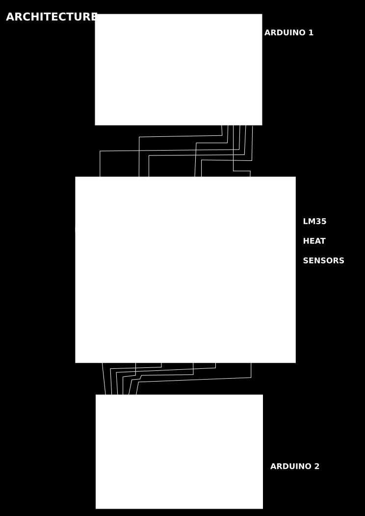
8 VTK has an extensive information visualization framework, has a suite of 3D interaction widgets, supports parallel processing, and integrates with various databases on GUI toolkits such as Qt and Tk. VTK is cross-platform and runs on Linux, Windows, Mac and Unix platforms. All VTK classes are wrapped with a Pythonic API supporting Traits. Classes are generated at install time on the installed platform. Elementary pickle support. Handles Numeric/numarray/scipy arrays/python lists transparently. Support for a pipeline browser, ivtk and a high-level mlab like module. Envisage plugins for a tvtk scene and the pipeline browser. tvtk is free software with a BSD style license. Demonstration of contour lines formation : Process : The demonstration will show the dynamic changes of contour values and its views. We are going to generate the contour lines from varying heat values, dynamically. Arranging many heat sensors in particular manner. Connect all the sensors into Arduino board to getting dynamic heat values of sensors. And arrange few moving Heat emitting object [say LED] which will generate the heat and is absorbed by the sensors and are converted into values using Arduino. The converted heat values are plotted dynamically and contours are generated. The variation in the distance between the Heat emitting source and each sensors will produce variations in heat values. This variation is considered as the altitude of the contour. Now, we have the values for latitude, longitude and altitude for the contour. When the Heat emitting source is moved dynamically between the sensors, the altitude values of each sensor will vary dynamically resulting in a dynamic contour. By this way, we can get the heat contour values dynamically and plotting those contour lines into computerised view. So we are going to view the dynamic changes of the contour values.

9 Detailed view of process : Take one square plywood. Set 12 (LM35) heat sensors on the plywood by the following manner. Fix four rows containing three sensors in each row of the board. The arrangement is as follows We can give six analog inputs into single arduino board. So we can connect six LM35 heat sensors into single arduino board. Using two arduino boards, we can get 12 heat sensors value.

10

11 Connect those two arduino boards into computer via two USB cables. By this way, we can get the heat sensors value (analog value) in the digital manner (digital value). Make arrangement to move one LED on the plywood by setting some path. We have to arrange the same to move more than one LED on the plywood board. Mark each sensors X-axis and Y-axis. While developing contour maps for this heat sensors values, the X-axis is set as Latitude and Y-axis is set as Longitude for each sensors. These values are assumed to be constants throughout the contour generation process. The heat value sensed by the each sensor are set as the altitude. In contour map, The altitude value is assumed to be the Z-axis which is a dynamic value. The point from the origin is plotted first and the altitude is used as the distance from that point to make a contour circle by assuming the point as the center. For example if (0,0) is the origin, then the point (x1,y1) is plotted from the origin. Then the altitude or heat value z1 is considered as the distance ( height in 3 dimension ) and point (x1,y1) as center to draw the contour circles. All the dynamically generated altitude values are fed into a program. The program inturn is embedded in Mayavi to produce a Dynamic 3 Dimensional View. The digital contour map lines varies dynamically when the Heat emitting source is moved randomly within the sensors range.

12

13

14 When two light emitting sources are placed on different positions over the heat sensor board,it produces a merged effect of contours with two high altitude points. The obtained result is depicted in the following figure.

15 The contours get transformed dynamically from one state to another when the heat source is placed in different positions over the heat sensors. The LED is moved over the path to make dynamic heat changing values which is sensed by all the sensors. The various transition states of LED are as follows.

16 The various transition states contour results are as follows.

17 APPLICATION OF CONTOUR ANALYSIS AND VISUALIZATION:

18 Software Requirements: Open Source Operating system Python language Mayavi2 TVTK Hardware Requirements: GPS Data Logger Few Arduino Boards Heat sensors ( LM35 ) Wires and Fixtures