NONPARAMETRIC REGRESSION TECHNIQUES

Transcription

1 NONPARAMETRIC REGRESSION TECHNIQUES C&PE 940, 28 November 2005 Geoff Bohling Assistant Scientist Kansas Geological Survey Overheads and other resources available at: 1

2 Modeling Continuous Variables: Regression In regression-style applications we are trying to develop a model for predicting a continuous-valued (numerical) response variable, Y, from one or more predictor variables, X, that is Y = f ( X ) In more classical statistical terminology, the X variables would be referred to as independent variables, and Y as the dependent variable. In the language of the machine learning community, the X s might be referred to as inputs and the Y as an output. We will limit our discussion to: Supervised learning: In which the response function, f, is learned based on a set of training data with known X & Y values. Deterministic X: That is, the noise or measurement error is considered to be strictly in the Y values, so that regression (in the general sense) of Y on X is the appropriate approach, rather than an approach aiming to minimize error in both directions (e.g., RMA regression). In other words, we are looking at the case where each observed response, y i, is given by y = f i x i ( ) + εi where x i is the corresponding vector of observed predictors and i ε is the noise or measurement error in the i th observation of y. 2

3 f is not known exactly and we instead substitute some convenient approximating function, f ˆ( X ;θ ), with a set of parameters, θ, that we can adjust to produce a reasonable match between the observed and predicted y values in our training data set. In typical statistical modeling, the form of ( X ) What constitutes a reasonable match is measured by an objective function, some measure of the discrepancy between y i and f ˆ( x i ;θ ) averaged over the training dataset. Ideally, the form of the objective function would be chosen to correspond to the statistical distribution of the error values, ε i, but usually this distribution is also unknown and the form of the objective function is chosen more as a matter of convenience. By far the most commonly used form is the sum of squared deviations between observed and predicted responses, or residual sum of squares: N ( i x i ) ( ) = y fˆ ( ; θ ) R θ. i= 1 If the errors are independent and distributed according to a common normal distribution, N ( 0,σ ), then the residual sum of squares (RSS) is in fact the correct form for the objective function, in the sense that minimizing the RSS with respect to θ yields the maximum likelihood estimates for the parameters. Because of its computational convenience, least squares minimization is used in many settings regardless of the actual form of the error distribution. 2 3

4 A fairly common variant is weighted least squares minimization, with the objective function R (?) = N i= 1 y fˆ σ i x i ( ; θ ) i 2 which would be appropriate if each error value was distributed according to ε i ~ N ( 0, σ i ). However, we rarely have external information from which to evaluate the varying standard deviations, σ i. One approach to this problem is to use iteratively reweighted least squares (IRLS), where the σ i values for each successive fit are approximated from the computed residuals for the previous fit. IRLS is more robust to the influence of outliers than standard least squares minimization because observations with large residuals (far from the fitted surface) will be assigned large σ i values and thus downweighted with respect to other observations. Probably the only other form of objective function (for regressionstyle applications) that sees much use is the sum of absolute (rather than squared) deviations: R N (?) = y fˆ ( ; θ ) i= 1 i x i which is appropriate when the errors follow an exponential distribution, rather than a normal distribution. Minimizing the absolute residuals (the L 1 norm) is also more robust to outliers than minimizing the squared residuals (the L 2 norm), since squaring enhances the influence of the larger residuals. However, L 1 minimization is difficult, due to discontinuities in the derivatives of the objective function with respect to the parameters. 4

5 So, the basic ingredients for supervised learning are: A training dataset: Paired values of y i and x i for a set of N observations. An approximating function: We must assume some form for the approximating function, f ˆ( X ;θ ), preferably one that is flexible enough to mimic a variety of true functions and with reasonably simple dependence on the adjustable parameters, θ. An objective function: We must also assume a form for the objective function which we will attempt to minimize with respect to? to obtain the parameter estimates. The form of the objective function implies a distributional form for the errors, although we may often ignore this implication. Even if we focus solely on the least squares objective function, as we will here, the variety of possible choices for f ˆ( X ;θ ) leads to a bewildering array of modeling techniques. However, all of these techniques share some common properties, elaborated below. Another important ingredient for developing a reliable model is a test dataset independent from the training dataset but with known y i values on which we can test our model s predictions. Without evaluating the performance on a test dataset, we will almost certainly be drawn into overfitting the training data, meaning we will develop a model that reproduces the training data well but performs poorly on other datasets. In the absence of a truly independent test dataset, people often resort to crossvalidation, withholding certain subsets from the training data and then predicting on the withheld data. 5

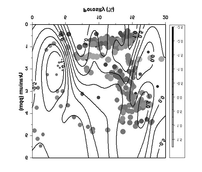
6 We will return to the Chase Group permeability example presented earlier by Dr. Doveton, except with a somewhat expanded (and messier) set of data. Here are the permeability data plotted versus porosity and uranium concentration. The circle sizes are proportional to the base 10 logarithm of permeability in millidarcies, with the permeability values ranging from md (LogPerm = -1.85) to 32.7 md (LogPerm = 1.52). The contours represent LogPerm predicted from a linear regression on porosity and uranium. The residuals from the fit, represented by the gray scale, range from to 1.27 with a standard deviation of For this dataset, the linear regression explains only 28% of the variation in LogPerm. 6

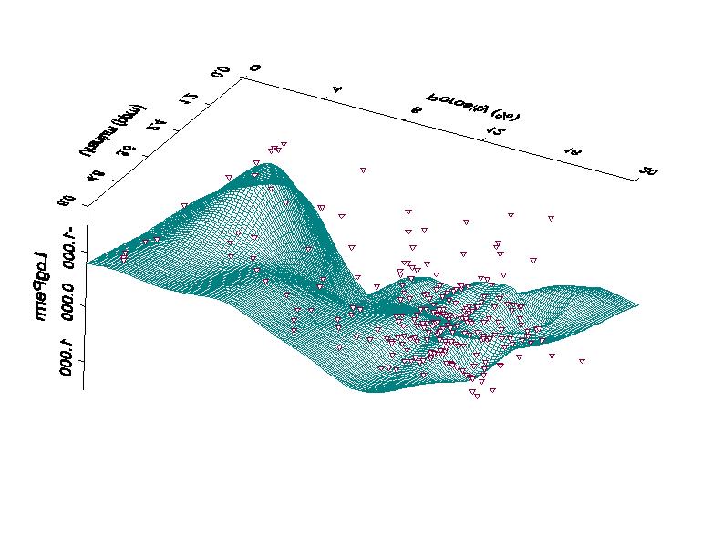
7 Here is a perspective view of the fitted surface followed by the prediction results versus depth: 7

8 To start thinking about different approaches for estimating Y = f ( X ), imagine sitting at some point, x, in the predictor space, looking at the surrounding training data points, and trying to figure out something reasonable to do with the y i values at those points to estimate y at x. Nearest-neighbor averaging: For each estimation point, x, select k nearest neighbors in training dataset and average their responses: Yˆ ( x) = 1 k Nk y ( x ) i ( x) N k means the neighborhood surrounding x containing k training data points. This approach is extremely simple. It is also very flexible in the sense that we can match any training dataset perfectly by choosing k = 1 (assuming there are no duplicate x i values with different y i values). Using one nearest neighbor amounts to assigning the constant value, y i, to the region of space that is closer to x i than to any other training data point the Thiessen polygon of x i. Why do we not just always use nearest-neighbor averaging? Because it does not generalize well, particularly in higher dimensions (larger numbers of predictor variables). It is very strongly affected by the curse of dimensionality... 8

9 The Curse of Dimensionality We are trying to map out a surface in the space of predictor variables, which has a dimension d equal to the number of predictor variables. Imagine that all the variables have been standardized to a common scale and that we are considering a hypercube with a side length of c in that common scale. The volume of this hypercube is given by d V = c So, the volume of the hypercube increases as a power of the dimension. This means that it becomes harder and harder for the training data to fill the volume as the dimensionality increases, and that the probability that an estimation point will fall in empty space far from any training data point increases as a power of the number of predictor variables. So, even a seemingly huge training dataset could be inadequate for modeling in high dimensions. Another way of looking at the curse of dimensionality is that if n training data points seem adequate for developing a onedimensional model (with a single predictor variable), then n d data points are required to get a comparable training data density for a d-dimensional problem. So, if 100 training data points were adequate for a 1-dimensional estimation problem, then = data points would be required to give a comparable density for a 10-dimensional problem. For any realistic training dataset, almost all of the predictor variable space would be far from the nearest data point and nearest-neighbor averaging would give questionable results. 9

10 A number of methods can be used to bridge the gap between a rigid global linear model and an overly flexible nearest-neighbor regression. Most of these methods use a set of basis or kernel functions to interpolate between training data points in a controlled fashion. These methods usually involve a large number of fitting parameters, but they are referred to as nonparametric because the resulting models are not restricted to simple parametric forms. The primary danger of nonparametric techniques is their ability to overfit the training data, at the expense of their ability to generalize to other data sets. All these techniques offer some means of controlling the trade-off between localization (representation of detail in the training data) and generalization (smoothing) by selection of one or more tuning parameters. The specification of the tuning parameters is usually external to the actual fitting process, but optimal tuning parameter values are often estimated via crossvalidation. Global regression with higher-order basis functions: The approximating function is represented as a linear expansion in a set h m x : of global basis or transformation functions, ( ) fˆ θ M ( x) = θ h ( x) m= 1 The basis functions could represent polynomial terms, logarithmic transformations, trigonometric functions, etc. As long as the basis functions do not have any fitting parameters buried in them in a nonlinear fashion, this is still linear regression that is, the dependence on the parameters is linear and we can solve for them in a single step using the standard approach for multivariate linear regression. The tuning here is in the selection of basis functions. For example, we could fit the training data arbitrarily well by selecting a large enough set of polynomial terms, but the resulting surface would flap about wildly away from data points. m m 10

11 Kernel Methods and Locally Weighted Regression: This involves weighting each neighboring data point according to a kernel function giving a decreasing weight with distance and then computing a weighted local mean or linear or polynomial regression model. So, this is basically the same as (smoothing) interpolation in geographic space, but now in the space of the predictor variables. The primary tuning parameter is the bandwidth of the kernel function, which is generally specified in a relative fashion so that the same value can be applied along all predictor axes. Larger bandwidths result in smoother functions. The form of the kernel function is of secondary importance. Smoothing Splines: This involves fitting a sequence of local polynomial basis functions to minimize an objective function involving both model fit and model curvature, as measured by the second derivative, expressed in one dimension as: RSS N 2 ( f, λ ) = { y f ( x )} + { f ( t) } i i λ i= i The smoothing parameter, λ, controls the trade-off between data fit and smoothness, with larger values leading to smoother functions but larger residuals (on the training data, anyway). The smoothing parameter can be selected through automated crossvalidation, choosing a value that minimizes the average error on the withheld data. The approach can be generalized to higher dimensions. The natural form of the smoothing spline in two dimensions is referred to as a thin-plate spline. The figures below show the optimal thin-plate spline fit for the Chase LogPerm data. The residuals from the fit range from to 1.42 with a standard deviation of 0.48 (compared to to 1.27 with a standard deviation of 0.61 for the linear regression fit). The spline fit accounts for 56% of the total variation about the mean, compared to 28% for the least-squares fit. 2 dt 11

12 12

13 Here are the measured and thin-plate spline predicted LogPerms versus depth: 13

14 Neural Networks: There is a variety of neural network types, but the most commonly applied form builds up the fitted surface as a summation of sigmoid (S-shaped) basis functions, each oriented along a different direction in variable space. A direction in variable space corresponds to a particular linear combination of the predictor variables. That is, for a set of coefficients, α, j = 1, K d, where j indexes the set of variables, plus an j, intercept coefficient, α 0, the linear combination α d 0 + α j = 1 represents a combined variable that increases in a particular direction in predictor space essentially a rotated axis in that space. For notational simplicity, we often add a column of 1 s to the set of predictor variables, that is, X 0 = 1 for every data point, so that the linear combination can be represented more compactly as d j = 0 jx j α = α X j X j The second expression shows the summation as the inner product of the coefficient vector and the variable vector. A typical neural network will develop some number, M, linear combinations like the one above meaning M different coefficient vectors, α m and pass each one through a sigmoid transfer function to form a new variable (basis function), Zm ( α X) = 1 ( 1+ ( α X) ) = σ exp m m 14

15 For continuous-variable prediction, the predicted output is then typically just a linear combination of the Z values: fˆ M = 0 m m ( X ) β + β Z = β Z = β Z m= 1 M m= 0 where again we have collapsed the intercept term into the coefficient vector by introducing Z 0 = 1. The complete expression for the approximating function is then fˆ M ( X ) = β mσ d m= 0 j = 0 α m m, j m X j 15

16 If we chose to use M = 4 sigmoid basis functions for the Chase example, the network could be represented schematically as: The input layer contains three nodes representing the bias term X 0 = 1 and the two input variables, porosity and uranium. The hidden layer in the middle contains the four nodes that compute the sigmoid transfer functions, Z m, plus the bias term Z 0 = 1. The lines connecting the input- and hidden-layer nodes represent the coefficients or weights α. The input to each hidden-layer m, j node (excluding the hidden-layer bias node) is one of the linear combinations of input variables and the output is one of the Z m values. The lines connecting the hidden layer node to the output 16

17 node represent the coefficients or weights β m, so the output node computes the linear combination β mz m, our estimate for LogPerm. M m = 0 Training the network means adjusting the network weights to minimize the objective function measuring the mismatch between predicted and observed response variables in a training data set. For continuous-variable prediction, this is usually the least-squares objective function introduced above. Adjusting the weights is an iterative optimization process involving the following steps: 0. Scale the input variables (e.g., to zero mean and unit standard deviation) so that they have roughly equal influence 1. Guess an initial set of weights, usually a set of random numbers 2. Compute predicted response values for the training dataset using current weights 3. Compute residuals or errors between observed & predicted responses 4. Backpropagate errors through network, adjusting weights to reduce errors on next go-round 5. Return to step 2 and repeat until weights stop changing significantly or objective function is sufficiently small Any of a number of algorithms suitable for large-scale optimization can be used -- meaning suitable for problems with a large number of unknown parameters, which are the network weights in this case. Given d input variables and M hidden-layer nodes (actually M+1 including the bias node) the total number of weights to estimate is N w = ( d + 1) M + ( M + 1) -- α s plus β s -- which can get to be quite a few parameters fairly easily. 17

18 Because we are trying to minimize the objective function in an N w - dimensional space, it is very easy for the optimization process to get stuck in a local minimum, rather than finding the global minimum, and typically you will get different results (find a different local minimum) starting from a different set of initial weights. Thus the neural network has a stochastic aspect to it and each set of estimated weights should be considered one possible realization of the network, rather than the correct answer. The most fundamental control on the complexity of the estimated function fˆ ( X ) is the choice of the number of hidden-layer nodes, M. (Usually the bias node is left out of the count of hidden-layer nodes.) We will refer to M as the size of the network. A larger network allows a richer, more detailed representation of the training data, with a smaller network yielding a more generalized representation. Here is the result of using a network with a single hidden-layer node just one sigmoid basis function for the Chase permeability example: 18

19 Here the network finds a rotated axis in Phi-U space oriented in the direction of the most obvious LogPerm trend, from lower values in the northwest to higher values in the southeast, and fits a very sharp sigmoid function practically a step function in this direction. If we use three basis functions, we might get a representation like the following: This looks like our first basis function plus one oriented roughly along the uranium axis, centered at about U = 1.2, and one oriented along an axis running from lower left to upper right, helping to separate out the low values in the southwest corner. 19

20 Quite often a term involving the magnitudes of the network weights is added to the objective function, so that the weights are now adjusted to minimize R ( α β ) + λj( α, β ) = y fˆ ( ; α, β ) N ( ) + λ( α ) i x i +, β i= 1 Minimizing this augmented function forces the network weights to be smaller than they would be in the absence of the second term, increasingly so as the damping or decay parameter, λ, increases. Forcing the weights to be smaller generally forces the sigmoid functions to be spread more broadly, leading to smoother representations overall. Here is the fit for a network with three hidden-layer nodes using a decay parameter of λ = 0. 01: You can see that the basis functions developed here are much less step-like than those developed before with no decay ( λ = 0). 20

21 Thus, the primary tuning parameters for this kind of neural network a single hidden-layer neural network with sigmoid basis functions are the size of network, M, and the decay parameter, λ. One strategy for choosing these might be to use a fairly large number of hidden-layer nodes, allowing the network to compute a large number of directions in predictor-variable space along which the response might show significant variation, and a large decay parameter, λ, forcing the resulting basis functions to be fairly smooth and also tending to reduce weights associated with directions of less significant variation. I have used crossvalidation to attempt to estimate the optimal values for M and λ for the Chase example, using an R-language script to run over a range of values of both parameters, M and λ and, for each parameter combination... Split the data at random into a training set (2/3 of the data) consisting of two-thirds of the data and a test set (remaining 1/3) Train a network on the training set Predict on the prediction set Compute the root-mean-squared residual on the prediction set. To account for the random variations due to the selection of training and testing data and due to the stochastic nature of the neural network, I have run the splitting-training-testing cycle 100 times over (different splits and different initial weights each time) for each parameter combination to yield... 21

22 The lines follow the median and upper and lower quartiles of the rms residual values for each parameter combination. The lowest median rmsr (0.341) occurs for a network size of 3 and a decay of 1 (Log10(decay) of 0), but the results for M = 10 and λ = 0.01 are slightly better in that the median rmsr is almost the same (0.342) and the upper and lower quartiles are a little lower. Using these values for M and λ and training on the whole dataset four different times leads to the following four realizations of the fitted surface: 22

23 The R 2 values (percent variation explained) for the above fits are 63% (upper left), 58% (upper right), 63% (lower left), and 62% (lower right). As with geostatistical stochastic simulation, the range of variation in results for different realizations of the network could be taken as a measure of the uncertainty in your knowledge of the true surface, f ( X ), leading to an ensemble of prediction results, rather than a single prediction for each value of X. You could of course average the predictions from a number of different network realizations. 23

24 Despite the varied appearance of the fitted surfaces vs. Phi-U, the results do not vary greatly at the data points and look much the same plotted versus depth: We would expect more variation at points in Phi-U space at some distance from the nearest training data point. However, in this case, predictions versus depth at a nearby prediction well also look quite similar for the four different networks. Reference T. Hastie, R. Tibshirani, and J. Friedman, The Elements of Statistical Learning: Data Mining, Inference, and Prediction, 2001, Springer. 24