Differential formulation of discontinuous Galerkin and related methods for compressible Euler and Navier-Stokes equations

Transcription

1 Graduate Theses and Dssertatons Graduate College 2011 Dfferental formulaton of dscontnuous Galerkn and related methods for compressble Euler and Naver-Stokes equatons Hayang Gao Iowa State Unversty Follow ths and addtonal works at: Part of the Aerospace Engneerng Commons Recommended Ctaton Gao, Hayang, "Dfferental formulaton of dscontnuous Galerkn and related methods for compressble Euler and Naver-Stokes equatons" (2011). Graduate Theses and Dssertatons Ths Dssertaton s brought to you for free and open access by the Graduate College at Iowa State Unversty Dgtal Repostory. It has been accepted for ncluson n Graduate Theses and Dssertatons by an authorzed admnstrator of Iowa State Unversty Dgtal Repostory. For more nformaton, please contact dgrep@astate.edu.

2 Dfferental formulaton of dscontnuous Galerkn and related methods for compressble Euler and Naver-Stokes equatons by Hayang Gao A dssertaton submtted to the graduate faculty In partal fulfllment of the requrements for the degree of DOCTOR OF PHILOSOPHY Maor: Aerospace Engneerng Program of Study Commttee: Z.J. Wang, Maor Professor Paul Durbn Hu Hu Halang Lu Alrc Rothmayer Iowa State Unversty Ames, Iowa 2011

3 TABLE OF CONTENTS LIST OF FIGURES LIST OF TABLES ABSTRACT v v v CHAPTER 1. General Introducton 1 Introducton 1 Dssertaton Organzaton 4 References 4 CHAPTER 2. The CPR Formulaton for Conservaton Laws 7 1. Revew of the Flux Reconstructon Method 7 2. Lftng Collocaton Penalty Formulaton 9 3. Numercal Results Conclusons 25 Reference 26 Appendx 27 CHAPTER 3. Dfferental Formulaton of Dscontnuous Galerkn and Related Methods for the Naver-Stokes Equatons 50 Abstract Introducton Governng Equatons and Numercal Formulatons Compact schemes for dscretzaton of the dffuson/vscous term Two-Dmensonal Fourer (Von Neumann) Analyss Numercal Results Conclusons 76

4 Acknowledgments 77 References 77 CHAPTER 4. A Study of Curved Boundary Representatons for 2D Hgh-order Euler Solvers 94 Abstract Introducton Interpolaton Polynomal Mappng (IP Mappng) Bezer Curve Based Geometry Mappng (Bezer Mappng) Numercal Tests Conclusons 103 Acknowledgement 104 References 104 CHAPTER 5. A Resdual-Based Procedure for hp-adaptaton on 2D Hybrd Meshes 115 Abstract Introducton Numercal Formulaton Mesh Adaptaton Numercal Tests Concluson 127 Acknowledgements 127 References 127 CHAPTER 6. General Concluson 137 ACKNOWLEDGEMENTS 138

5 v LIST OF FIGURES CHAPTER 2. The CPR Formulaton for Conservaton Laws Fgure 1. Soluton ponts (squares) and flux ponts (crcles) for k = Fgure 2. Soluton and flux ponts n a smplex for k = 1, 2, and Fgure 3. One of the weghtng functons for the spectral volume method, k = Fgure 4. Soluton and flux ponts for the 3 rd order CP scheme on hybrd meshes. 40 Fgure 5. Transformaton of a quadrlateral element to a standard element. 40 Fgure 6. Transformaton of a Curve Boundary Trangular Element to a Standard Element. 40 Fgure 7. Regular and Irregular "10x10x2" Computatonal Grds. 41 Fgure 8. Coarse mxed mesh for accuracy study. 41 Fgure 9. Trangular Mesh and 2 nd, 3 rd and 4 th Order Results for Flow around a Cylnder. 43 Fgure 10. Mxed Mesh #1 and 2nd, 3rd and 4th Order Results for Flow around a Cylnder. 45 Fgure 11. Mxed Mesh #2 and 4th Order Results for Flow around a Cylnder. 47 Fgure 12. The Mxed Grd n the Smulaton of Flow around NACA0012 Arfol. 47 Fgure 13. 2nd Order Soluton of the Flow around NACA0012 Arfol. 48 Fgure 14. 3rd Order Soluton of the Flow around NACA0012 Arfol. 48 Fgure 15. 4th Order Soluton of the Flow around NACA0012 Arfol. 49 Fgure 16. Entropy Error on the Upper Wall of NACA0012 Arfol. 49 CHAPTER 3. Dfferental Formulaton of Dscontnuous Galerkn and Related Methods for the Naver-Stokes Equatons Fgure 1. Soluton ponts (squares) and flux ponts (crcles) for k = Fgure 2. Soluton ponts for the 3rd order CPR scheme on hybrd meshes. 86 Fgure 3. Transformaton of a quadrlateral element to a standard element. 86 Fgure 4. Irregular trangular mesh for Posson s equaton on [0,1] X[0,1]. 87 Fgure 5. Meshes for potental flow over a cylnder. 87 Fgure 6. Soluton contours for potental flow over a cylnder (BR2, 3rd order, 20X20 mesh). 88

6 v Fgure 7. Convergence hstory of potental flow over a cylnder (4th order, 40x40 meshes): (a) quadrlateral mesh (b) trangular mesh. 88 Fgure 8. Mxed mesh used for Couette flow. 89 Fgure 9. Mxed mesh around an NACA0012 arfol. 89 Fgure 10. Mach number contours of flow around an NACA 0012 arfol. 90 Fgure 11. Cf on the upper surface of NACA0012 arfol for BR2, I-contnuous, nteror penalty and CDG. 91 Fgure 12. 4th order convergence hstory of lamnar flow over NACA0012 arfol n terms of (a) teratons (b) CPU tme. 92 Fgure 13. Mxed mesh for unsteady flow around a cylnder. 91 Fgure 14. Mach number contours for unsteady flow around a cylnder. 93 CHAPTER 4. A Study of Curved Boundary Representatons for 2D Hgh-order Euler Solvers Fgure 1. Smplfed quadratc and cubc trangular elements wth one curve sde. 106 Fgure 2. Bezer curves of varous degrees. 106 Fgure 3. Schematc of quadratc Bezer curve. 106 Fgure 4. Geometry mappng for a quadrlateral cell wth one curved sde. 107 Fgure 5. Constructon of a cubc Bezer curve boundary segment. 107 Fgure 6. (a) Tangental drectons due to a pont of nflecton and (b) resulted transformaton. 107 Fgure 7. Problematc nodes (n whte) for P-2 Bezer curves. 108 Fgure 8. (a) The tangental drectons where the curve boundary ends. (b) The fx to the sngularty problem by extrapolatng t 2 wth Fgure 9. Approxmatons of a crcular segment by dfferent approaches, the errors enlarged by 50 tmes. 108 Fgure 10. Comparson of the P-5 and P-3 Bezer representatons, wth errors enlarged by 20,000 tmes. 109 Fgure 11. Computatonal mesh used for flow over a cylnder. 109 Fgure 12. Entropy error dstrbutons on the cylnder wall, 6th order LCP. 110 Fgure 13. L2 entropy errors computed wth 2nd 6th order schemes. 110

7 v Fgure 14. A 4X6 mesh around the cylnder. 111 Fgure 15. Entropy error dstrbutons on a coarse mesh for the flow over a cylnder. 111 Fgure 16. A mxed mesh for NACA0012 test case. 112 Fgure 17. Entropy errors on the upper wall of NACA0012 arfol wth a 6th order scheme, computed wth exact geometry nformaton. 112 Fgure 18. Entropy error feld near the leadng edge of NACA0012 arfol wth the 6th order scheme. 113 Fgure 19. Entropy errors on the upper wall of NACA0012 arfol wth a 6th order scheme, computed wthout exact geometry nformaton. 114 CHAPTER 5. A Resdual-Based Procedure for hp-adaptaton on 2D Hybrd Meshes Fgure 1. The confguraton of soluton ponts (square) and flux ponts (crcle) of p-2 and p-3 CPR method. 130 Fgure 2. Demonstraton of a mortar face procedure for a p-nterface. 130 Fgure 3. The computatonal doman and mesh for the subsonc bump flow. 130 Fgure 4. The result of p-adaptaton for subsonc bump flow, fadapt Fgure 5. The Ma contours for the bump flow after p-adaptaton. 131 Fgure 6. The L2 entropy error from p-adaptaton and unform p-refnement. 132 Fgure 7. (a) Hybrd mesh for subsonc flow over NACA 0012 arfol. (b) Ma contour of the ntal 2nd order soluton. 132 Fgure 8. P-adpataton results for the subsonc flow over NACA0012 arfol. 133 Fgure 9. Ma contour of subsonc arfol flow after p-adaptaton. 133 Fgure 10 (a) L2 entropy error (b) drag coeffcent error for the subsonc arfol flow. 134 Fgure 11. Intal mesh for the transonc arfol flow. 135 Fgure 12. hp-adaptaton results for the transonc arfol flow. 135 Fgure 13. Densty contours for the transonc arfol flow after hp-adaptaton. 136

8 v LIST OF TABLES CHAPTER 2. The CPR Formulaton for Conservaton Laws Table 1. Test of CP-DG for ut ux u y 0, wth u0( x, y) sn ( x y), at t 1, for trangular mesh. 34 Table 2. Test of CP-SV for u u u 0, wth u0( x, y) sn ( x y), at t 1 t x y for trangular mesh. 35 Table 3. Test of CP-DG for ut uux uuy 0, wthu0( x, y) sn ( x y), at t. 1, for trangular mesh wth LP approach. 36 Table 4. Test of CP-DG for ut uux uuy 0, wthu0( x, y) sn ( x y), at t. 1, for trangular mesh wth CR approach. 37 Table 5. Test of CP-DG for Euler Equatons wth Vortex Propagaton Case, for trangular and mxed meshes. 38 CHAPTER 3. Dfferental Formulaton of Dscontnuous Galerkn and Related Methods for the Naver-Stokes Equatons Table 1. Mnmum egenvalues, orders of accuracy, and errors for schemes on a square mesh. 80 Table 2. Mnmum egenvalues, orders of accuracy, and errors for schemes on a trangular mesh. 81 Table 3. Accuracy results of Posson s equaton wth regular quadrlateral mesh (Interor Penalty s dentcal to BR2). 81 Table 4. Accuracy results of Posson s equaton wth rregular trangular mesh. 82 Table 5. Accuracy results for a potental flow over a cylnder wth quadrlateral meshes (Interor Penalty s dentcal to BR2). 82 Table 6. Accuracy results for a potental flow over a cylnder wth trangular meshes. 83 Table 7. Accuracy results of Couette flow wth hybrd mesh. 84 Table 8. Flow over a NACA0012 arfol pressure drag coeffcents C D,p. 84 Table 9. Flow over a NACA0012 arfol frcton drag coeffcents C D,f. 84 Table 10. Flow over a NACA0012 arfol separaton pont on the upper surface. 85 Table 11. P-refnement study for unsteady flow around a cylnder. 85

9 v ABSTRACT A new approach to hgh-order accuracy for the numercal soluton of conservaton laws ntroduced by Huynh and extended to smplexes by the current work s renamed CPR (correcton procedure or collocaton penalty va reconstructon). The CPR approach employs the dfferental form of the equaton and accounts for the umps n flux values at the cell boundares by a correcton procedure. In addton to beng smple and economcal, t unfes several exstng methods ncludng dscontnuous Galerkn (DG), staggered grd, spectral volume (SV), and spectral dfference (SD). The approach s then extended to dffuson equaton and Naver-Stokes equatons. In the dscretzaton of the dffuson terms, the BR2 (Bass and Rebay), nteror penalty, compact DG (CDG), and I-contnuous approaches are used. The frst three of these approaches, orgnally derved usng the ntegral formulaton, were recast here n the CPR framework, whereas the I-contnuous scheme, orgnally derved for a quadrlateral mesh, was extended to a trangular mesh. The current work also ncludes a study of hgh-order curve boundares representatons. A new boundary representaton based on the Bezer curve s then developed and analyzed, whch s shown to have several advantages for complcated geometres. To further enhance the effcency, the capablty of h/p mesh adaptaton s developed for the CPR solver. The adaptaton s drven by an effcent mult-p a posteror error estmator. P-adaptaton s appled to smooth regons of the flow feld whle h-adaptaton targets the non-smooth regons, dentfed by accuracy-preservng TVD marker. Several numercal tests are presented to demonstrate the capablty of the technque.

10 1 CHAPTER 1. General Introducton Introducton In today s CFD applcatons, almost all the producton solvers are based on second order methods. These solvers are capable of delverng desgn-qualty soluton to a lot of flow problems wth reasonable computng cost, thus have made a great mpact n many ndustry felds. However, for certan flow problems, second order schemes are held back by ther low accuracy and dsspatve nature. Such examples would nclude the wave propagaton n computatonal aero-acoustcs, complex flow structures n large eddy smulaton (LES) and drect numercal smulaton (DNS) of turbulence flows, and vortex domnated flows such as helcopter vortex blade nteracton. Hgh-order methods, on the other hand, show great promse n delverng much better soluton qualty wth comparable computng costs, and therefore have become the popular choce for applcatons that requre hgh accuracy and low dsspaton. For a hgh-order method to be appled to a wde varety of real lfe flow problems, there are several features to be desred. Frst of all, the method should be robust, most mportantly stable. To be appled to complex geometres, the method should be able to handle unstructured meshes, even mxed/hybrd meshes. A compact stencl s also very benefcal, for mplct schemes and parallel computng. Last but not the least, the deal hgh-order method should be effcent, preferably n a dfferental formulaton rather than an ntegral one. Numerous hgh-order methods for compressble flows have been developed n the last two decades. Here, we focus only on those that employ a polynomal to approxmate the soluton n each cell or element, and the polynomals collectvely form a functon whch s dscontnuous across cell boundares. These methods generally feature a compact stencl due to ther local soluton reconstructon, whch s also deal for use n unstructured meshes. Commonly used methods of ths type nclude dscontnuous Galerkn (DG) [3,4,7-9], staggered-grd (SG) [20], spectral volume (SV) [31-35], and spectral dfference (SD) [22-24]. Among these, DG and SV are usually formulated va the ntegral form of the equaton, whereas SG and SD, the dfferental one. Among these methods, DG s arguably the leader due to ts guaranteed stablty from ts weghted resdual formulaton, whle for other

11 2 methods, a unversal framework for stablty of all orders of accuracy n arbtrary types of element s stll lackng. Although the DG method s mathematcally well-defned and straghtforward, ts mplementaton mght be qute nvolved due to ts ntegral form. Huynh (2007) [18] ntroduced an approach to hgh-order accuracy called flux reconstructon (FR). The approach solves the equatons n dfferental form. It evaluates the frst dervatve of a dscontnuous pecewse polynomal functon by employng the straghtforward dervatve estmate together wth a correcton whch accounts for the umps at the nterfaces. The FR framework unfes several exstng methods: wth approprate correcton terms, t recovers DG, SG, SV and SD methods. In the current work, the FR method s extended to 2D and 3D smplexes, and appled to 2D mxed meshes. Intally ths method s called the lftng collocaton penalty (LCP) method. Later, due to ther tght connecton, the FR and LCP methods are renamed correcton procedures va reconstructon or CPR. The CPR formulaton does not nvolve numercal ntegratons; the mass matrx nverson s bult-n and therefore not needed; as a consequence, the approach s smpler and generally results n schemes more effcent than those by quadrature-based formulatons. The CPR formulaton s then extended to dffuson and Naver-Stokes equatons, whch nvolves the second dervatves. There are many approaches for the extenson. Here, only the ones wth a compact stencl are consdered. The four schemes of compact stencl employed are BR2 (Bass and Rebay) [5], compact DG or CDG [25], nteror penalty [11,16], and I-contnuous (the value and dervatve are contnuous across the nterface) [19]. The BR2 scheme, an mprovement of the non-compact BR1 [3], s the frst successful approach of ths type for the Naver-Stokes equatons. The CDG scheme s a modfcaton of the local DG or LDG [10] to obtan compactness for an unstructured mesh. The nteror penalty scheme s employed here wth a penalty coeffcent usng correcton functon [19]. The I-contnuous approach s hghly accurate for lnear problems on a quadrlateral mesh. Ncknamed poor man s recovery, t can be consdered as an approxmaton to the recovery approach of Van Leer and Nomura [27]. In the current work, all the four approaches are cast n the deferental formulaton of the CPR method for 2D mxed meshes. The capablty of the CPR framework for dffuson and Naver-Stokes equatons s

12 3 demonstrated. Comparsons are also made for the four approaches mentoned above n terms of accuracy and convergence. Another topc related to the hgh-order methods s the representaton of the curve wall boundares. As hgh-order methods become ncreasngly mature for real world applcatons, the hgh-order boundary treatment becomes a crtcal ssue. In manstream fnte volume solvers, the wall boundary of the geometry s usually represented by pecewse straght segments or planar facets. However, ths lnear boundary representaton s far from suffcent for hgh-order methods. The curvlnear element was ntroduced by Gordon and Hall [13-14] to solve the problem, whch was also used by Koprva [20] n the staggeredgrd method. Both Bass and Rebay [4], Wang and Lu [36] also addressed the mportance of curve boundary representaton n ther work on hgh-order methods. Prevously, hghorder boundary s represented by extra nterpolaton ponts added to a boundary face. The current work ntroduces a new mappng approach based on the Bezer curve, whch s able to reconstruct the boundary wth a contnuous slope, wthout ntroducng any sharp corners. Examnaton of ths technque shows ts advantage n reducng spurous entropy producton for complex geometres. Adaptve soluton technques are also developed wth the CPR method to acheve greater effcency. H-refnement stands for local mesh subdvson, whle p-refnement local polynomal degree enrchment. It has been shown that p-adaptaton s superor n regons where the soluton s smooth [21], whle h-adaptaton s preferred n non-smooth regons such as flow dscontnutes, where hgh-order methods become less effectve. Combned h/p-adaptaton offers even greater flexblty for complex problems. For an h/p-adaptaton scheme, two ndcators needs to be computed: a local error ndcator to serve as the adaptaton crtera, and a local smoothness ndcator, used to decde whether h- or p- adaptaton should be appled to a certan regon. Error ndcators are based error estmaton approaches, such as gradent or feature based error estmate [6,15], resdual-based error estmate [1,2,26], and adont-based error estmate [12,17,28-30]. In the present study, a resdual-based approach usng a mult-p error estmaton s adopted as the error ndcator. Ths error ndcator nvolves no ad-hoc parameters. It s also much more effcent to compute compared to the adont-based approach. The accuracy-preservng TVD (AP-TVD)

13 4 marker [37] s employed n the present study as the non-smoothness ndcator to dentfy the non-smooth regons. Dssertaton Organzaton The rest of ths dssertaton s organzed as follows. Chapter 2, The CPR formulaton for conservaton laws s on the dervaton of the CPR method and ts applcaton on conservaton laws ncludng Euler equatons for mxed meshes. Chapter 3, Dfferental Formulaton of Dscontnuous Galerkn and Related Methods for the Naver-Stokes Equatons s a paper submtted to the Journal of Scentfc Computng for publcaton. The paper detals the extenson the CPR formulaton to dffuson and Naver-Stokes equatons. I am the prmary author of the paper, responsble for most of the work and wrtng except Secton 4 on Fourer analyss. Chapter 4, A study of curved boundary representatons for 2D hgh order Euler solvers s a paper publshed n the Journal of Scentfc Computng. The paper s about the curved boundary representaton approach based on Bezer curve. I am the prmary author of the paper, responsble for most of the work and wrtng. Chapter 5, A Resdual-Based Procedure for hp-adaptaton on 2D Hybrd Meshes s a paper publshed n the 49th AIAA ASM conference proceedngs. The paper elaborates the development of h/p adaptaton procedure wth the CPR flow solver. I am the prmary author of the paper, responsble for most of the work and wrtng. Chapter 6 s devoted to general conclusons. References [1] M. Answorth, J.T. Oden, A unfed approach to a posteror error estmaton usng element resdual methods, Numer. Math. 65 (1993) [2] T.J. Baker, Mesh adaptaton strateges for problems n flud dynamcs. Fnte Elem Anal Des 1997;25: [3] F. Bass and S. Rebay, A hgh-order accurate dscontnuous fnte element method for the numercal soluton of the compressble Naver Stokes equatons. J. Comp. Phys. 1997;131(1): [4] F. Bass and S. Rebay, Hgh-order accurate dscontnuous fnte element soluton of the 2D Euler equatons, J. Comput. Phys. 138, (1997). [5] F.Bass and S. Rebay, GMRES Dscontnuous Galerkn Soluton of the Compressble Naver-Stokes Equatons. In Karnadaks Cockburn and Shu, edtors, 208. Sprnger, Berln, 2000.

14 5 [6] M. J. Berger and P. Collela, Local adaptve mesh refnement for shock hydrodynamcs, J. Comput. Phys., vol. 82, pp , [7] B. Cockburn and C.-W. Shu, TVB Runge-Kutta local proecton dscontnuous Galerkn fnte element method for conservaton laws II: general framework, Mathematcs of Computaton 52, (1989). [8] B. Cockburn, S.-Y. Ln and C.-W. Shu, TVB Runge-Kutta local proecton dscontnuous Galerkn fnte element method for conservaton laws III: one-dmensonal systems, J. Comput. Phys. 84, (1989). [9] B. Cockburn and C.-W. Shu, The Runge-Kutta dscontnuous Garlerkn method for conservaton laws V: multdmensonal systems, J. Comput. Phys., 141, , (1998). [10] B. Cockburn and C.-W. Shu, The local dscontnuous Galerkn methods for tme-dependent convecton dffuson systems, SIAM J. Numer. Anal., 35(1998), pp [11] V. Doleší, On the dscontnuous Galerkn method for numercal soluton of the Naver-Stokes equatons, Int. J. Numer. Methods Fluds, 45: , [12] M. B. Gles and N. A. Perce. Adont equatons n CFD: Dualty, boundary condtons and soluton behavor. AIAA paper , [13] W. J. Gordon and C. A. Hall, "Constructon of Curvlnear Co-ordnate Systems and Applcatons to Mesh Generaton," Int. J. Num. Meth. Engng., 7 (1973), pp [14] W. J. Gordon and C. A. Hall, Transfnte element methods and blendng functon nterpolaton over curved element domans. Numer. Math. 21(1973), [15] R. Harrs and Z.J. Wang, Hgh-order adaptve quadrature-free spectral volume method on unstructured grds, Computers & Fluds 38 (2009) [16] R. Hartmann and P. Houston, Symmetrc nteror penalty DG methods for the ncompressble Naver- Stokes Equatons I: Method formulaton. Int. J. Numer. Anal. Model., 1:1-20. [17] R. Hartmann and P. Houston. Adaptve dscontnuous Galerkn fnte element methods for the compressble Euler equatons. J. Comput. Phys., 183: , [18] H.T. Huynh, A flux reconstructon approach to hgh-order schemes ncludng dscontnuous Galerkn methods, AIAA Paper [19] H.T. Huynh, A Reconstructon Approach to Hgh-Order Schemes Includng Dscontnuous Galerkn for Dffuson, AIAA Paper [20] D.A. Koprva and J.H. Kolas, A conservatve staggered-grd Chebyshev multdoman method for compressble flows, J. Comp. Physcs, 125(1996), pp [21] Y. L, S. Premansuthan and A. Jameson, Comparson of h- and p-adaptatons for spectral dfference method, AIAA [22] Y. Lu, Vnokur M, and Wang ZJ. "Dscontnuous Spectral Dfference Method for Conservaton Laws on Unstructured Grds," n Proceedngs of the 3rd Internatonal Conference on Computatonal Flud Dynamcs, Toronto, Canada, July

15 6 [23] Y. Lu, Vnokur M, and Wang ZJ. "Dscontnuous Spectral Dfference Method for Conservaton Laws on Unstructured Grds," Journal of Computatonal Physcs Vol. 216, pp (2006). [24] G. May and A. Jameson, A spectral dfference method for the Euler and Naver-Stokes equatons, AIAA paper No , [25] J. Perare and P.-O. Persson, The compact dscontnuous Galerkn (CDG) method for ellptc problems, SIAM J. Sc. Comput., Vol. 30, No. 4 (2008) pp [26] Shh, T.I-P. and Qn, Y., A Posteror Method for Estmatng and Correctng Grd-Induced Errors n CFD Solutons Part 1: Theory and Method, AIAA Paper [27] B. van Leer and S. Nomura, Dscontnuous Galerkn for Dffuson, AIAA Paper [28] D.A. Vendtt, D.L. Darmofal, Adont error estmaton and grd adaptaton for functonal outputs: Applcaton to quas-one-dmensonal flow. J Comput. Phys. 2000;164: [29] D.A. Vendtt, D.L. Darmofal, Ansotropc grd adaptaton for functonal outputs: applcaton to twodmensonal vscous flows, J. of Comp. Phys, 187 (2003) [30] L. Wang and D. Mavrpls, Adont-based h-p Adaptve Dscontnuous Galerkn Methods for the Compressble Euler Equatons, AIAA [31] Z.J. Wang, Spectral (Fnte) volume method for conservaton laws on unstructured grds: basc formulaton, J. Comput. Phys. Vol. 178, pp , [32] Z.J. Wang, Hgh-order methods for the Euler and Naver-Stokes equatons on unstructured grds, Journal of Progress n Aerospace Scences, Vol. 43, pp. 1-47, [33] Z.J. Wang and Y. Lu, Spectral (fnte) volume method for conservaton laws on unstructured grds : one-dmensonal systems and partton optmzaton, Journal of Scentfc Computng, Vol. 20, No. 1, pp (2004). [34] Z.J. Wang and Y. Lu, Spectral (fnte) volume method for conservaton laws on unstructured grds : one-dmensonal systems and partton optmzaton, Journal of Scentfc Computng, Vol. 20, No. 1, pp (2004). [35] Z.J. Wang, L. Zhang and Y. Lu, Spectral (Fnte) Volume Method for Conservaton Laws on Unstructured Grds IV: Extenson to Two-Dmensonal Euler Equatons, Journal of Computatonal Physcs Vol. 194, No. 2, pp (2004). [36] Z.J. Wang, Y. Lu, Extenson of the spectral volume method to hgh-order boundary representon, J. Comput. Phys. 211 (2006) [37] M. Yang and Z.J. Wang, A parameter-free generalzed moment lmter for hgh-order methods on unstructured grds, AIAA

16 7 CHAPTER 2. The CPR Formulaton for Conservaton Laws 1. Revew of the Flux Reconstructon Method Ths revew presents the essental dea of the flux reconstructon developed by Huynh [4]. Consder the followng scalar conservaton law Q F( Q) 0, (1.1) t x where Q s the state varable and F s the flux. The computatonal doman [a, b] s dscretzed nto N elements, wth the th element defned by V x, x ]. Each [ 1/ 2 1/ 2 element can be transformed nto the standard element [-1, 1] usng a lnear transformaton. The DOFs at the th element are the nodal values of the state varable Q, at k+1 soluton ponts, x,, = 1,..., k+1. Then the soluton s approxmated by the followng degree k Lagrange nterpolaton polynomal k 1 h Q ( x) Q ( x) L( x) Q,, (1.2) 1 where L (x) s the Lagrange polynomal or shape functon. Gven ths numercal soluton, the flux at every pont s well defned,.e., F( Q h ( x)). For non-lnear conservaton laws, F( Q h ( x)) may not be a polynomal. Instead, F( Q h ( x)) s approxmated by the followng degree k flux polynomal k 1 h F ( x) L( x) F( Q ( x, )). (1.3) 1 Obvously, f the flux s a lnear functon of Q, F (x) s dentcal to F( Q h ( x)). Snce we do not explctly enforce contnuty at element nterfaces, the state varable s dscontnuous across the nterfaces. In order to update the DOFs, a new flux functon F ˆ ( x ) s reconstructed, whch must satsfy the followng crtera: F ˆ ( x ) s a degree k+1 polynomal,.e., one order hgher than the soluton polynomal;

17 8 F ˆ ( x ) s close to F (x) n some sense. In other words, some norm of the dfference Fˆ ( x) F ( x) s mnmzed; At both ends of the element, the flux takes on the value of the Remann fluxes,.e., ~ ~ F ˆ ( x ) F( Q ( x ), Q ( x )) F 1/ 2 1/ 2 1 1/ 2 1/ 2 1 1/ 2 1/ 2 1/ 2 ~ ~ F ˆ ( x ) F( Q ( x ), Q ( x )) F, 1/ 2 ~ where F ( Q, Q ) s any Remann flux gven the two dscontnuous solutons at the left and rght of the nterface. Once ths flux functon s found, the DOFs are updated usng the followng dfferental equaton Q t, Fˆ ( x x, ) 0. (1.4) Obvously the above crtera do not unquely defne F ˆ ( x ). As a matter of fact, only two condtons are gven. We need k extra condtons to defne the degree k+1 polynomal F ˆ ( x ). Usng specal polynomals such as the Radau and Legendre polynomals, Huynh [4] successfully recovered F ˆ ( x ) for the DG, SG (or SD/SV) methods, at least for lnear conservatons laws. The reconstructed flux s frst re-wrtten as Fˆ ( x) F ( x) ( x), (1.5) where (x) s a correcton flux polynomal, whch should be as close as possble to 0. The correcton s then further expressed to satsfy the two end condtons ~ ~ x) [ F F ( x )] g ( x) [ F F ( x )] g ( ), (1.6) ( 1 / 2 1/ 2 L 1/ 2 1/ 2 R x where g L (x) and g R (x) are both degree k+1 polynomals called correcton functons, and they satsfy g ( x L g ( x R 1/ 2 1/ 2 ) 1, ) 0, g ( x L g ( x R 1/ 2 1/ 2 ) 0 ) 1. (1.7) Eq. (1.4) then becomes Q, t h F ( x x, ) ~ [ F 1/ 2 F ( x 1/ 2 )] g ( x L, ~ ) [ F 1/ 2 F ( x 1/ 2 )] g ( x R, ) 0. (1.8)

18 9 Because of symmetry, we only need to consder g L (x), or smply g(x). It s more convenent to consder the correcton functon n the standard element g ( ) on [-1, 1]. Many correcton functons were presented n [4], correspondng to dfferent numercal methods. Several schemes are descrbed next. 1. If g s the rght Radau polynomal, the resultng scheme s actually the DG method! 2. If g has Chebyshev-Lobatto ponts as ts nteror roots, the resultng scheme s the SG method or the SD/SV method n 1D. The scheme, however, s mldly unstable, whch was also found by Van den Abeele et al [8]. 3. If g has a vanshng dervatve at the rght boundary as well as at the nteror Legendre- Lobatto ponts, the method results n a remarkably smple, yet stable scheme f one chooses the Legendre-Lobatto ponts as the soluton ponts snce the correctons for the nteror soluton ponts vansh! Huynh named ths scheme the g 2 scheme. 4. If g has the Legendre-Gauss ponts as ts nteror roots, the scheme s stable. Ths suggests that usng the Legendre-Gauss ponts and the two end ponts as flux ponts results n a stable SG method n 1D. As mentoned earler, the FR method has some remarkable propertes. Its DG formulaton looks lke a pseudo-dg. However, t s dentcal to the real DG formulaton! The natural queston next s how about smplex elements and other cell types? Ths s the focus of the current study. As can be seen above, reconstructng the full Fˆ ( x, ) s actually not necessary, snce eventually what s needed s the dervatve F ˆ ( ) / x, x,.e. the last two terms n the lefthand-sde of (1.8). Therefore, a more effcent approach s pursued when attemptng to extend ths method to 2D and 3D smplexes. The followng secton descrbes the basc dea. 3. Lftng Collocaton Penalty Formulaton 3.1 Basc Idea Rewrte the hyperbolc conservaton law as

19 10 where F ( F x, F y ) Q F( Q) 0, (2.1) t s the flux vector. Assume that the computatonal doman s dscretzed nto N non-overlappng trangular elements { V }. Let W be an arbtrary weghtng functon. The weghted resdual form of (2.1) on element V can be easly derved by multplyng (2.1) wth W and ntegratng over V to obtan Let Q Q F( Q) WdV WdV WF( Q) nds W F( Q) dv 0. t t (2.2) V V V V h Q be an approxmate soluton to Q at element. We assume that the soluton belongs h to the space of polynomals of degree k or less,.e., Q P k (whose dmenson s m), wthn each element wthout contnuty requrement across element nterfaces. In addton, we requre that the numercal soluton h Q must also satsfy (2.2),.e., h Q WdV h h WF ( Q ) nds W F ( Q ) dv 0. t (2.3) V V V A common Remann flux s used to replace the normal flux to provde element couplng,.e., where n h h n h h F ( Q ) F( Q ) n F ( Q, Q, n), (2.4) h Q s the soluton outsde the current element V. Then (2.3) becomes h Q WdV n h h h WF ( Q, Q, n ) ds W F ( Q ) dv 0. t (2.5) V V V Applyng ntegraton by parts to the last term on the LHS of (2.5), we obtan h Q WdV h n h h n h W F ( Q ) dv W F ( Q, Q, n ) F ( Q ) ds 0. t (2.6) V V V The last term on the left sde of (2.6) can be vewed as a penalty term,.e., penalzng the k normal flux dfferences. Introduce a correcton feld P, whch s determned from a lftng operator W dv W[ F] ds, (2.7) V V

20 11 where ~ ~ n h h n h [ F] F ( Q, Q, n) F ( Q ) (2.6), we obtan s the normal flux dfference. Substtutng (2.7) nto h Q h F( Q ) WdV 0. t (2.8) V k 1 If the flux vector s a lnear functon of the state varable, then F Q P. In ths case, the terms nsde the square bracket are all elements of P k. Because the test space s selected to ensure a unque soluton, Eq. (2.8) s equvalent to Q t h h FQ ( ) 0, (2.9) k For non-lnear conservaton laws, FQ s usually not an element of k result, we approxmate t by ts proecton onto P V, denoted by to defne ths proecton s Eq. (2.14) then reduces to d F Q P V. As a. One way F Q W V F Q WdV (2.10) V V Q t FQ ( ) 0. (2.11) Wth the ntroducton of the correcton feld, and a proecton of F Q for non-lnear conservaton laws, we have reduced the weghted resdual formulaton to a dfferental formulaton, whch nvolves no ntegrals. The performance of ths formulaton of course hnges on how effcently the correcton feld can be computed. To get a sense of ts form, lettng W = 1 n (2.7), we obtan or dv [ F] ds, (2.12) V V 1 [ F] ds V, (2.13) fv f

21 12 1 [ ~ F] ds, V f V f (2.13) ~ where s the volume averaged. We can assume that the flux dfference [F] s a ~ degree k polynomal on face f, and can be determned based on values of [ ] at a set of F f, l flux ponts usng a Lagrange nterpolaton, as shown n Fgure 1. Then the face ntegral can be computed exactly usng a quadrature formula such as 1 w [ Fˆ ] S, (2.14) l f, l f V f V l where w l s the quadrature weght for the surface ntegral, and S f s the area of face f. Next let the degrees-of-freedom (DOFs) be the solutons at a set of ponts, named soluton ponts (SPs), as shown n Fgure 1. Then equaton (2.9) must be true at the SPs,.e., r, Q t h, h, FQ ( ) 0, (2.15) h h where F( Q ) F( Q ) r,. ~ Let s examne (2.7) more carefully. If [F] s assumed to be degree k polynomals along the cell faces, and that the trangle has straght face, the correcton feld computed explctly n the followng form,, f, l f, l f V f V l can be 1 [ F] S, (2.16) where are constant coeffcents ndependent of the soluton, but dependent on the, f, l weghtng functon W. Substtutng (2.16) nto (2.15) we obtan the followng formulaton h Q, 1 F( Q ) [ F] S 0 t. (2.17) h, f, l f, l f V f V l Obvously, ths s a collocaton-penalty formulaton. In addton, a lftng operator s used to completely remove the weghtng functons, whch are used to compute the constant lftng coeffcents, f, l.

22 13 h Next, we focus on how to compute the proecton ( FQ ( )), a brute force mplementaton based on Eq.(2.11) requres hgh-order ntegral quadrature, and thus s expensve. Two more effcent approaches are presented here. Approach 1. Lagrange polynomal approach Based on the soluton at an SP, the flux vector at each SP can be computed. Then a degree k Lagrange nterpolaton polynomal for the flux vector s used to approxmate the nonlnear flux vector. SP where ( ) SP, F Q I F Q L r F Q (2.18) k L r s the Lagrange polynomal based on the soluton ponts r, proecton s computed usng SP, k. After that, the F Q I F Q L F Q (2.19) In ths case ( FQ ( )) s a degree k-1 polynomal, whch also belongs to P k. Numercal tests ndcate a slght loss of accuracy wth the LP approach. Approach 2. Chan rule (CR) approach It s recognzed that the dvergence of the flux vector can be computed analytcally gven the approxmate soluton by usng the chan rule,.e. where F Q F Q Q,, Q,, (2.20) FQ (, ) s the flux Jacoban matrces, whch can be computed analytcally, then the Q proecton s approxmated by the Lagrange nterpolaton polynomal of the flux vector dvergence at the soluton ponts,.e. SP F Q L r F Q,. (2.21) Numercal experments ndcate that the CR approach s much more accurate than the LP approach. Now that the CPR formulaton s complete, let s examne (2.17) a bt further. It s obvously a collocaton-lke formulaton, wth penalty-lke terms to provde the couplng

23 14 between elements. However, wth a specal choce of scheme coeffcents, f, l, we can show that (2.17) s equvalent to the DG method, at least n the lnear case. From (2.7), t s easy to show that s unquely defned once proper test functons W and the flux ponts are gven. Therefore, the locaton of the soluton ponts does not affect the soluton polynomal Q h h (r) (although Q, obvously depends on the locaton of r, ) or the correcton polynomal. Therefore, the most effcent choce s to make the soluton ponts concde wth the flux ponts because no data nterpolatons are then needed for flux computatons. Any convergent nodal sets wth enough ponts at the element nterface are good canddates, e.g., those found n [1,3,9]. Fgure 2 shows the locaton of the DOFs for k = 1, 2 and Connecton between the CP and DG, SV and SD Methods Let s frst express the soluton and the correcton n terms of the DOFs,.e., where Q L Q, (2.22) h h, L, (2.23), L s the Lagrange polynomal based on the soluton ponts. In the DG method, the weghtng functon W s set to be one of the Lagrange polynomal nto (2.7), we obtan the followng equatons Lk V Lk, dv Ll [ F] f, l f V f l L. Substtutng W L ˆ ds, k = 1,..., m. (2.24) The unknowns n (2.24), can be easly solved n terms of the normal flux umps at the flux ponts ˆ ] [ F f, l, and the coeffcents, f, l be determned, whch are constant for any straght-sded trangles. The coeffcents for the DG schemes are ncluded n Appendx 1. In the case of k = 1, the coeffcents for the frst the soluton pont are { }. Therefore, the formula for the correcton s 1 (2.5[ F ] 0.5[ F ] ) S ( 1.5[ F ] 1.5[ F ] ) S (0.5[ F ] 2.5[ F ] ) S. (2.25),1 1,1 1,2 1 2,1 2,2 2 3,1 3,2 3 V Although all the flux ponts concde wth the soluton ponts, as shown n Fgure 2, t s necessary to dstngush flux ponts accordng to whch face they are located on because

24 15 each face has a dfferent normal drecton. In addton, the flux ponts on each face are numbered ndependently for easy dentfcaton and mplementaton. In the SV method, the weghtng functon s 1 wthn a partton of the element, and 0 elsewhere, for example, as shown n Fgure 3 n the case of k = 1. Repeatng the same wth all the parttons, we obtan agan m equatons for m unknowns,, whch can be unquely solved. The coeffcents for several SV schemes are also ncluded n Appendx 1. The coeffcents for the frst soluton pont of the second order SV method are { }, correspondng to the followng formula 1 (2[ F ] 0.2[ F ] ) S ( 0.7[ F ] 0.7[ F ] ) S (0.2[ F ] 2[ F ] ) S.,1 1,1 1,2 1 2,1 2,2 2 3,1 3,2 3 V (2.26) In the SD method, the correcton feld s computed based on the drect dfferental of a reconstructed flux vector,.e., ˆ h [ F F( Q )], (2.27) where Fˆ s a reconstructed flux vector from the Remann fluxes at the element nterface and fluxes n the nteror of the element. The components of Fˆ are polynomals of degree k+1, one degree hgher than the soluton polynomal, so that s of degree k. The dervaton s a lttle more nvolved than those for the DG and SV method. We found that only on an equlateral trangular grd can the SD method degenerate nto the CPR form gven n (2.16). Ths s not surprsng because the SD method s generally not only dependent on the normal fluxes at element nterfaces, but also on the tangental fluxes. The k = 1 lnear case has the followng coeffcents at the frst soluton pont { }, resultng n the followng formula, f, l,1 1,1 1 2,1 2,2 2 3,2 3 V 1 2[ F ] S ( 0.5[ F ] 0.5[ F ] ) S 2[ F ] S. (2.28) Note that the coeffcents are qute dfferent for the DG, SV and SD methods. These schemes have been numercally confrmed to be equvalent to the DG, SV and SD methods for lnear conservaton laws.

25 16 Snce the DG method s the most popular among the hgh-order methods for compressble flow, let s compare the CPR formulaton wth the DG method n terms of cost, for the case of k = 2. Here are the man operatons n the conventonal DG methods wth surface and volume quadratures: Reconstruct the state varables at 6 volume quadrature ponts and 9 surface quadrature ponts. Compute the analytcal fluxes at the 6 volume quadrature ponts, and Remann fluxes at the 9 surface quadrature ponts. Multply the fluxes wth the quadrature weghts, and the weghtng functons or ther gradents to form the resdual; Multply the resdual by the nverse of the mass matrx. The man operatons n the CPR method nclude: Compute the analytcal fluxes at the 6 soluton ponts, and 9 Remann fluxes at surface flux ponts. Multply the fluxes wth the dfferental quadrature weghts to form the dvergence of the flux vector, and add the penalty terms to form the resdual. Due to the specal choce of DOFs, the reconstructon cost s completely avoded, and the mass matrx s avoded n the CPR method. In addton, t s not necessary to store the weghtng functons or ther gradents. Therefore, the CPR formulaton s more effcent n both memory and CPU tme. 3.3 Conservaton Constrants for Lftng Coeffcents It should not be a surprse that more choces of coeffcents are possble, and may even be benefcal, for example, to allow the largest possble tme step, or preserve certan range of frequency contents better than the standard methods. However, snce we are dealng wth conservaton laws, the schemes should be conservatve wth any coeffcents. In order to guarantee conservaton, the ntegral conservaton laws must be satsfes,.e., V h Q dv n h h F ( Q, Q, n ) ds 0 t (2.29) V

26 17 whch corresponds to (2.6) wth W = 1. Ths means the CPR method s fundamentally conservatve at the element level. Next let s derve the conservatve constrants whch must be satsfed by the lftng coeffcents. Assume the followng quadrature s used for the volume ntegral Q dv V v Q, (2.30) V h h, where v are the quadrature weghts for the volume ntegral. Then the frst term n (2.29) becomes h h Q Q, 1 h dv V v V v F ( Q, ), f, l[ F ] S f, l f. t (2.31) V t V f V l Snce the quadrature rule s exact for degree k (or less) polynomals, we have Accordng to (2.29), we obtan. (2.32) V v F( Q ) F( Q ) dv F ( Q ) ds h h n h, V V 1 n n h V v, f, l[ F] f, ls f F F ( Q ) ds w l[ F] f, ls f. V (2.33) f V l V f V l The LHS of (2.33) can be smplfed nto v [ F] S v [ F] S. (2.34), f, l f, l f, f, l f, l f f V l f V l Comparng (2.34) and (2.33), we obtan the followng condton w v. (2.35) l, f, l Ths s also the necessary and suffcent condton for the CPR formulaton to be conservatve. In the lnear case, w 1/ 2 and v 1/ 3, the conservaton condton s then whch s satsfed by the DG, SV and SD schemes. 3.4 Extenson to Mxed Grds l 3 2 3, (2.36) It s obvous that (2.9) s vald for arbtrary types of elements besdes trangles. For vscous flow problems, t s often advantageous to have quadrlateral cells or prsmatc cell near 1, f, l

27 18 sold walls to resolve vscous boundary layers. In the present study focusng on 2D problems, we address mxed grds ncludng both trangular and quadrlateral meshes. As mentoned earler, t s straghtforward to extend Huynh s FR approach [4] to quadrlateral meshes. In order to smplfy the mplementaton, we assume the polynomal degree k to be the same for both the trangular and quadrlateral meshes. Furthermore, the flux ponts along the element nterfaces are requred to match each other, as shown n Fgure 4. In order to acheve an effcent mplementaton, all elements are transformed from the physcal doman ( x, y) nto a standard square element (, ) [-1,1]x[-1,1] as shown n Fgure 5. The transformaton can be wrtten as x x, (2.37) K M (, ) y 1 y where K s the number of ponts used to defne the physcal element, x, y ) are the ( Cartesan coordnates of those ponts, and M (, ) are the shape functons. For the transformaton gven n (2.37), the Jacoban matrx J takes the followng form ( xy, ) x x J (, ) y y. (2.38) For a non-sngular transformaton, ts nverse transformaton must also exst, and the Jocoban matrces are related to each other accordng to ( x, y) x (, ) x y 1 J y Therefore the metrcs can be computed accordng to x y / J, y x / J, x y / J, y x / J. (2.39) The governng equatons n the physcal doman are then transformed nto the computatonal doman (standard element), and the transformed equatons take the followng form ~ Q F F 0. (2.40) t where ~ Q J Q (2.41).

28 19 ) ( y y x x F F J F (2.42) ) ( y y x x F F J F. (2.43) Let ), ( ),, ( y x y x J S J S. Then we have S F F S F F,. In our mplementaton, J and S S, are stored at the soluton ponts. Wthn the th element, the soluton polynomal s a tensor product of 1D Lagrange polynomals,.e., , ; ) ( ) ( ), ( k l k l h l h L L Q Q, (2.44) where h l Q, ; are the state varables at the soluton pont (,l), wth the ndex n drecton and l the ndex n drecton, ) ( L and ) ( l L are 1D Lagrange polynomals n and drectons. Based on the reconstructed soluton ), ( h Q, the fluxes can be defned usng ) ( ), ( h h Q F Q F. Agan, one can also choose to represent the fluxes wth Lagrange nterpolaton polynomals n the followng form: , ; ) ( ) ( ), ( k l k l l L L F F, (2.45a) , ; ) ( ) ( ), ( k l k l l L L F F. (2.45b) The reconstructed fluxes are only element-wse contnuous, but dscontnuous across cell nterfaces. Agan Remann fluxes are computed at all four element nterfaces n the normal drectons, whch are the same or opposte drectons of S or S. For example, at nterfaces 1, and 1, the outgong normals are S S n / 1. (2.46a) S S n / 1. (2.46b) Therefore the Remann flux correspondng to F s computed accordng to S n Q Q F F n ) ), 1, ( ), 1, ( ( ~ ) 1, ( ~, (2.47a) S n Q Q F F n ) ), (1, ), (1, ( ~ ) (1, ~. (2.47b) Fnally the DOFs are updated usng the followng equaton

29 20 0. ) (,1)] (,1) ( ~ [ ) ( 1)], ( 1), ( ~ [ ) ( )] (1, ) (1, ~ [ ) ( )] 1, ( ) 1, ( ~ [ ), ( ), ( ~,,,,,,,,,,,,,,,,, ; l R l l l L l l l R l l l L l l l l l l l g F F g F F g F F g F F F F t Q (2.48) Note that, the correcton s done n a one dmensonal manner. For example, 2, ] ~ [ f F n Fgure 4 only corrects the DOFs at the sold squares. In other words, for quadrlateral cells, the operatons are actually one-dmensonal, makng the method more effcent per DOF than for trangular cells. The flux dvergence n (2.48) can be obtaned usng ether the LP or the CR approach. Numercal tests show that the CR approach gves more accurate and unform results. In the present mplementaton, we choose ether the DG or the g 2 schemes from the FR famly [4]. The g 2 scheme s the smplest possble. For all nteror soluton pont, the correcton vanshes. In the case shown n Fgure 4, the correcton for 2, ] ~ [ f F needs only to apply to the soluton pont concdng wth the flux locaton! Recall that the soluton ponts for the g 2 approach are the Legendre-Lobatto ponts. Therefore, the soluton ponts for all trangular elements at each edge are also Legendre-Lobatto ponts along the edge tangental drecton to make the nterface treatment as smple as possble. 3.5 Extenson to Curved Boundary Cells In second-order CFD solvers, curved boundares are represented wth lnear lne segments or planar facets. However, for hgh order solvers, ths smple representaton may not be able to preserve the geometry well enough snce the computatonal grd s normally much coarser, and may even make the solvers unstable. The approach to solve the problem s to represent the curved boundary wth hgher order polynomals nstead of the lnear representaton for second order solvers. The change of boundary representatons actually does not alter the soluton technque, snce all we need to do s to transform the curved boundary cell nto a standard cell. For example, for a boundary element shown n Fgure 6, a quadratc transformaton s used to transform t to a standard element. After the transformaton, the governng equaton becomes (2.40) on the standard element, whch has straght edges. The CPR formulaton s

30 21 then appled to the transformed equaton on the standard rght trangle. Eq. (2.17) for the transformed equaton on a standard trangle becomes h Q, F ( Q ) 2 [ F ] S 0 t, (2.47) h,, f, l f, l f f V l where superscrpt mean the varables or operatons evaluated on the computatonal ~ doman. For example, [ ] are the normal umps of the transformed fluxes across the F f, l faces of the standard trangle. Note that when solvng Equaton (2.40), ~ Q J Q s the state vector, and s assumed to be a degree k polynomal n the computatonal doman nstead of Q. As a result, the dervatve of Q should be calculated n the followng way, Q 1 JQ J x J x x Q 1 JQ J y J y y Q, (2.48a) Q. (2.48b) Snce the transformaton s quadratc, J x and J y are non-zero. It s obvous that when the cell has straght faces, J s a constant n the element. Then (2.48) reduces to the usual dervatve evaluaton. For a quadrlateral cell, the curved boundary cells are treated n a smlar manner. Each cell s transformed to a standard square wth a hgh-order transformaton, and then (2.40) s solved n the computatonal doman on a standard element. 3. Numercal Results 3.1 Accuracy Study wth 2D Scalar Conservaton Laws Lnear Wave Equaton In ths case, we test the accuracy of the CPR method usng the two-dmensonal lnear equaton:

31 22 u u u 0, t x y 1 x 1, 1 y 1, u( x, y,0) u0 ( x, y), perodc boundary condton. (3.1) The ntal condton s u ( x, y) sn ( x ). Two types of computatonal meshes are 0 y used, one regular and the other rregular as shown n Fgure 7. The fner meshes are generated recursvely by cuttng each coarser grd cell nto four fner grd cells. The tme ntegraton schemes used are the TVD or SSP Runge-Kutta schemes of thrd or 4 th order accuracy [5,2,6]. The results are made tme step ndependent so that the spatal error s the domnant error source. The numercal smulaton s carred untl t = 1. The smulaton was ntalzed by nectng the exact ntal soluton nto the soluton ponts. The numercal solutons at the three vertces of all the trangular elements are then used to compute the L 2 error norm to measure the global soluton qualty Error L2 N 3 h e 2 ( Q, Q, ) 1 1 3N, (3.2) where e Q denotes the exact soluton. For lnear wave equatons, all DG formulatons are dentcal, so are all SV formulatons. In the present CPR famly, the DG and SV formulatons are denoted by CPR-DG and CPR-SV respectvely. Tables 1 and 2 present the computed errors wth both formulatons on the regular and rregular meshes. Note that optmal accuracy has been acheved for all the test cases, on both the regular and rregular meshes. The SD formulaton cannot completely degenerate nto the CPR, and therefore s not consdered n the accuracy study. 2D Burgers Equaton In ths case, we test the accuracy of the CPR method on the two-dmensonal non-lnear wave equaton: u t 2 u / 2 x 2 u y / 2 0, 1 1 u( x, y,0) sn ( x y), x 1, 1 y 1, perodc boundary condton. (3.3)

32 23 The ntal soluton s smooth. Due to the non-lnearty of the Burgers equaton, dscontnutes wll develop n the soluton. At t = 0.1, the exact soluton s stll smooth. The numercal smulaton s therefore carred out untl t = 0.1 on both the regular and rregular grds. In Table 3-4, we present the L 1, L2 and L errors produced usng the CPR-DG formulaton on rregular grds, wth both LP (Lagrange Polynomal, Table 3) approach and CR (chan-rule, Table 4) approach used n evaluatng the nteror flux dervatves and the accuracy of these two approaches s compared. Note n Table 3 and 4 that CR approach s better n every case and every norm of error consdered here, snce t not only produces smaller error, but also shows more consstency and better accuracy, especally for L norm, n grd refnement studes. 3.2 Accuracy Study wth Vortex Evoluton Problem Ths s an dealzed problem for the Euler equatons n 2D used by Shu [3]. The mean flow s {, u, v, p} = {1, 1, 1, 1}. An sotropc vortex s then added to the mean flow,.e., wth perturbatons n u, v, and temperature T = p/, and no perturbaton n entropy S = p/ : 2 0.5(1 r ) ( u, v) e ( y, x), 2 2 ( 1) 2 1r T e, 2 8 S 0, where r x y, and the vortex strength = 5. If the computatonal doman s nfntely bg, the exact soluton of the Euler equatons wth the above ntal condtons s ust the passve convecton of the sotropc vortex wth the mean velocty (1, 1). In the numercal smulaton, the computatonal doman s taken to be [-5,5]x[-5,5], wth characterstc nflow and outflow boundary condtons mposed on the boundares. The numercal smulatons were carred out untl t = 2 on two dfferent grds, one rregular trangular mesh and one mxed mesh as shown n Fgure 7b and Fgure 8. The fner rregular grds are generated recursvely by cuttng each coarser grd cell nto four fner grd cells, whle all mxed meshes are generated ndependently, whch s manly composed of rregular quadrlateral cell, wth a small number of trangular cells. For rregular trangular mesh, two tests are performed. In Test 1, the nteror flux dervatves are

33 24 evaluated usng the LP (Lagrange polynomal) approach, whle n Test 2, these dervatves are evaluated by the CR (chan rule) approach descrbed n Secton 3.1. For the mxed mesh, only the latter approach s used. The CP-DG scheme s used for trangular cells whle the FR-DG scheme s used for quadrlateral cells. For tme ntegraton, a 3-stage Runge-Kutta explct scheme s used for tme marchng n all the cases. In Table 5, the L 2 norms of densty error at the soluton ponts are presented for all three tests from 2 nd order to 4 th order. Comparng the results n Table 6, we fnd that the CR approach s much more accurate n every case. The CR approach not only produced the smaller errors, but also demonstrated more consstent order of accuracy n the grd refnement studes. In addton, the CPR method performs very well on the mxed grds, achevng the optmal order of accuracy on relatvely poor qualty meshes. Because the CR approach n evaluatng the nteror flux dervatves s shown superor to the LP approach, t s used n all other test cases presented next. 3.3 Flow Over a Cylnder To test the new method for curved wall boundares, the case of a subsonc flow at Mach 0.3 around a half-cylnder s smulated. For the curve wall, a quadratc wall representaton s used n the solver. Three grds are used, one trangular mesh, and two mxed mesh as shown n Fgure 9(a), 10(a) and 11(a). The frst mxed mesh s composed of regular quadrlateral cells near the wall boundary and rregular trangular cells elsewhere, whle the second mxed mesh s composed of fully mxed rregular quadrlateral and trangular cells, and has poor grd qualty near the wall. The 2 nd - 4 th order CPR-DG scheme s used for trangular cells and the 2 nd - 4 th order FR- DG scheme used for the quadrlateral cells. For tme ntegraton, a LU-SGS mplct solver s used wth 1 st order tme accuracy, and all the cases converged to machne zero. The 2 nd, 3 rd and 4 th order results for the 3 grds are shown n Fgure 9, 10 and 11. Note that whle 2 nd order solutons show some dscontnutes, smooth solutons are obtaned wth all the grds for 3 rd and 4 th order cases, even on Mxed Mesh #2, and all the 4 th order solutons agree well wth each other. The results show that the CPR method performs well for mxed mesh wth curve boundary elements, snce the smooth solutons across trangular

34 25 and quadrlateral cells can be obtaned as the order of accuracy ncreases. Furthermore, the hgh order solutons are also smooth near the curved boundary. 3.4 Flow Around NACA 0012 Arfol As the fnal test case for a more realstc geometry, the subsonc flow around a NACA 0012 arfol s smulated wth CPR method, wth 2 nd, 3 rd and 4 th order accuracy. The flow condtons are Mach = 0.3 and angle of attack = 5 degrees. Agan curved boundares are represented wth the quadratc polynomals. The mesh, shown n Fgure 12, s composed of regular quadrlateral mesh near the arfol whle rregular trangular and quadrlateral mesh elsewhere, wth a total of 1,510 cells. The outer boundary of the computatonal doman s about 20 chords from the center of the arfol. Agan, the CPR-DG scheme s used for trangular cells and FR-DG s used for quadrlateral cells. A LU-SGS solver s used for tme ntegraton, and all the cases converge to machne zero. The pressure and Mach number solutons from the 2 nd, 3 rd and 4 th order smulaton are shown n Fgure The computed soluton for the 2 nd order case s not smooth, wth vsble ump across cell boundares, due to the coarse mesh, whle n the 3 rd and 4 th order cases, the soluton s qute smooth. Besdes, the 3 rd and 4 th order results are almost the same wth only a lttle dfference near the tralng edge, whch ndcates a converged soluton. In Fgure 16, the entropy errors along the upper surface of the arfol s plotted for the 2 nd, 3 rd and 4 th order results as an ndcator of the accuracy. Obvously the error shows an exponental convergence as the order of the smulaton s ncreased. 4. Conclusons In the present study, a remarkably smple and effcent flux reconstructon formulaton developed by Huynh for conservaton laws s extended and generalzed to smplex cells. Instead of reconstructng the flux polynomal, the correcton polynomal s reconstructed usng a lftng operator. The new formulaton s therefore called a lftng collocaton penalty method. The fnal formulaton s free of weghtng functons, although the lftng coeffcents are dependent on the weghtng functons. Through a udcous selecton of soluton and flux ponts, soluton reconstructons can be completely avoded. In addton, the mass matrx s always dentty for arbtrary meshes. Furthermore, lke the FR formulaton, the dscontnuous Galerkn, spectral volume, and n a specal case the spectral

35 26 dfference method can all be recovered by the present formulaton wth dfferent choces of lftng coeffcents. The present formulaton s more effcent than the orgnal DG formulaton based on volume and surface ntegral quadratures. For non-lnear flux functons, the CPR method allows the nteror flux dervatves to be computed exactly usng the chan rule approach, whch appears to be benefcal n soluton accuracy. The extenson to curved boundares can be conducted n a straghtforward manner because no surface or volume ntegrals are requred. Numercal tests have been carred out for lnear, nonlnear scalar conservaton laws, and the 2D Euler equatons, for mxed trangular and quadrlateral meshes. These tests fully demonstrate the capablty of the CPR formulaton. The extenson to the Naver-Stokes equatons, and to 3D mxed meshes ncludng tetrahedral, prsmatc, pyramdal, and hexahedral cells s currently carred out, and wll be reported n future publcatons. Reference [1] Q. Chen and I. Babuska, Approxmate optmal ponts for polynomal nterpolaton of real functons n an nterval and n a trangle, Comput. Methods Appl. Mech. Engrg, 128, (1995). [2] Gottleb S, Shu CW. Total varaton dmnshng Runge Kutta schemes. Math Comput 1998;67: [3] Hesthaven JS. From electrostatcs to almost optmal nodal sets for polynomal nterpolaton n a smplex, SIAM J. Numer. Anal. Vol. 35 No. 2 (1998) [4] H.T. Huynh, A flux reconstructon approach to hgh-order schemes ncludng dscontnuous Galerkn methods, AIAA Paper [5] C.-W. Shu, Total-Varaton-Dmnshng tme dscretzatons, SIAM Journal on Scentfc and Statstcal Computng 9, (1988). [6] Spter, R.J., and Ruuth, S.J., (2002). A new class of optmal hgh-order strong-stabltypreservng tme dscretzaton methods. SIAM J. Numer. Anal. 40, [7] K Van den Abeele and C Lacor. An accuracy and stablty study of the 2D spectral volume method, submtted to Journal of Computatonal Physcs. [8] K Van den Abeele, C. Lacor and Z.J. Wang, "On the connecton between the spectral volume and the spectral dfference method, Journal of Computatonal Physcs, Volume 227, No. 2, pp (2007). [9] Z.J. Wang and Y. Lu, Spectral (fnte) volume method for conservaton laws on unstructured grds : one-dmensonal systems and partton optmzaton, Journal of Scentfc Computng, Vol. 20, No. 1, pp (2004).

36 27 Appendx The Coeffcents to Compute the Correcton at Soluton Ponts 2 nd Order Schemes Fgure A-1. Soluton ponts for k = 1 element Pont Locatons n Computatonal Doman Pont , f, l for 2 nd Order CPR-DG Scheme 1 Accordng to Equaton (2.14),,,, [ F], S V arbtrary trangular cell n the physcal doma,. When appled to a f l f l f f V l V s the area of cell, [ F] f, l s the normal flux dfference computed at l -th soluton ponts along face/edge f, and smply the length of face/edge f. As a conventon, faces are drectonal, and the 1 2 S f s drecton of the faces s such that the nteror of the cell s always on the left sde of any face. Faces are numbered that wthn any cell, Face 1 are the face from Pont 1 to Pont 2, Face 2 from Pont 2 to 3, and Face 3 from Pont 3 to 1, and here Pont 1, 2 and 3 are always the three vertces of the trangle. The numberng setup for 2 nd order scheme s shown n Fgure A-2.

37 28 [F] 3,1 [F] 2,2 3 Face 3 Face 2 [F] 3,2 Face [F] 2,1 [F] 1,2 [F] 1,2 Fgure A-2. Numberng Setup to Compute the Correcton for k = 1 element And, f, l are lsted n the followng table: f, l (1,1) 2.5 (1,2) 0.5 (2,1) -1.5 (2,2) -1.5 (3,1) 0.5 (3,2) The table shows that and from symmetry, 1 (2.5[ F ] A 0.5[ F ] A 1.5[ F ] A 1.5[ F ] A,1 1,1 1 1,2 1 2,1 2 2,2 2 V 0.5[ F] A 2.5[ F] A ) 3,1 3 3,2 3 1 (0.5[ F ] A 2.5[ F ] A 2.5[ F ] A 0.5[ F ] A,2 1,1 1 1,2 1 2,1 2 2,2 2 V 1.5[ F] A 1.5[ F] A ) 3,1 3 3,2 3

38 29 1 ( 1.5[ F ] A 1.5[ F ] A 0.5[ F ] A 2.5[ F ] A,3 1,1 1 1,2 1 2,1 2 2,2 2 V 2.5[ F] A 0.5[ F] A ) 3,1 3 3,2 3, f, l for 2 nd Order CPR-SV Scheme f, l, f, l for 2 nd Order CPR-SD Scheme f, l (1,1) 2.0 (1,2) 0.2 (2,1) -0.7 (2,2) -0.7 (3,1) 0.2 (3,2) 2.0 (1,1) 2.0 (1,2) 0.0 (2,1) -0.5 (2,2) -0.5 (3,1) 0.0 (3,2) rd Order Schemes Fgure A-3. Soluton ponts for k = 2 element

39 30 Pont Locatons n Computatonal Doman Pont , f, l for 3 rd Order CPR-DG Scheme f, l 1 4 (1,1) (1,2) (1,3) (2,1) (2,2) (2,3) (3,1) (3,2) (3,3)

40 31, f, l for 3 rd Order CPR-SV Scheme (wth the partton SV3P by Van den Abeele[7]) f, l 1 4 (1,1) (1,2) (1,3) (2,1) (2,2) (2,3) (3,1) (3,2) (3,3) The 4 th Order Schemes Fgure A-4. Soluton ponts for k = 3 element

41 32 Pont Locatons n the Computatonal Doman Pont , f, l for 4 th Order CPR-DG Scheme f, l (1,1) (1,2) (1,3) (1,4) (2,1) (2,2) (2,3) (2,4) (3,1) (3,2) (3,3) (3,4)

42 33, f, l for 4 th Order CPR-SV Scheme (wth the partton SV4P by Van den Abeele[7]) f, l (1,1) (1,2) (1,3) (1,4) (2,1) (2,2) (2,3) (2,4) (3,1) (3,2) (3,3) (3,4)

43 34 Table 1. Test of CP-DG for ut ux u y 0, wth u0( x, y) sn ( x y), at t 1, for trangular mesh. Polynomal degree k 1 Grd sze Regular Mesh Irregular Mesh L 2 error Order L 2 error Order 10x10x2 2.44e e-2-20x20x2 5.89e e x40x2 1.46e e x80x2 3.64e e x10x2 1.88e e-3-20x20x2 2.38e e x40x2 2.98e e x80x2 3.73e e x10x2 7.55e e-4-20x20x2 4.94e e x40x2 3.08e e x80x2 1.93e e x10x2 7.53e e-7-20x20x2 1.18e e x40x2 1.85e e

44 35 Table 2. Test of CP-SV for ut ux u y 0, wth u0( x, y) sn ( x y), at t 1 for trangular mesh. Polynomal degree k 1 Grd sze Regular Mesh Irregular Mesh L 2 error Order L 2 error Order 10x10x2 5.94e e-1-20x20x2 1.45e e x40x2 3.72e e x80x2 9.23e e x10x2 2.84e e-3-20x20x2 3.71e e x40x2 4.73e e x80x2 5.97e e x10x2 1.04e e-4-20x20x2 6.53e e x40x2 4.11e e x80x2 2.57e e

45 36 Table 3. Test of CP-DG for ut uux uuy 0, wthu0( x, y) sn ( x y), at t. 1, for trangular mesh wth LP approach. Polynomal degree k 1 Grd sze L1 error Order L 2 error Order L error Order 10x10x2 2.12e e e-2-20x20x2 6.96e e e x40x2 2.19e e e x80x2 6.79e e e x10x2 4.36e e e-2-20x20x2 7.76e e e x40x2 1.26e e e x80x2 1.93e e e x10x2 5.41e e e-3-20x20x2 4.70e e e x40x2 3.56e e e x80x2 2.65e e e x10x2 1.15e e e-4-20x20x2 2.94e e e x40x2 6.37e e e x80x2 1.23e e

46 37 Table 4. Test of CP-DG for ut uux uuy 0, wthu0( x, y) sn ( x y), at t. 1, for trangular mesh wth CR approach. Polynomal degree k 1 Grd sze L1 error Order L 2 error Order L error Order 10x10x2 1.34e e e-2-20x20x2 3.64e e e x40x2 9.39e e e x80x2 2.37e e e x10x2 1.57e e e-2-20x20x2 2.10e e e x40x2 2.62e e e x80x2 3.15e e e x10x2 1.31e e e-3-20x20x2 8.64e e e x40x2 5.70e e e x80x2 3.63e e e x10x2 2.42e e e-4-20x20x2 5.08e e e x40x2 8.17e e e x80x2 1.43e e e

47 38 Table 5. Test of CP-DG for Euler Equatons wth Vortex Propagaton Case, for trangular and mxed meshes. Polynomal degree k 1 Grd sze Irregular Trangular Mesh - Test 1 Irregular Trangular Mesh - Test 2 Mxed Mesh L 2 error Order L 2 error Order L 2 error Order 10x10x2 2.01e e e-2-20x20x2 6.67e e e x40x2 1.73e e e x80x2 4.84e e e x10x2 7.14e e e-3-20x20x2 1.07e e e x40x2 1.60e e e x80x2 2.29e e e x10x2 1.79e e e-4-20x20x2 1.40e e e x40x2 9.75e e e x80x2 6.96e e e

48 39 ˆ ] [ F f,3 ˆ ] [ F f,2 ˆ ] [ F f,1 Fgure 1. Soluton ponts (squares) and flux ponts (crcles) for k = 2. (a) k = 1 (b) k = 2 (c) k = 3 Fgure 2. Soluton and flux ponts n a smplex for k = 1, 2, and Fgure 3. One of the weghtng functons for the spectral volume method, k = 1.

49 40 ˆ ] [ F f,3 ˆ ] [ F f,2 ˆ ] [ F f,1 Fgure 4. Soluton and flux ponts for the 3 rd order CP scheme on hybrd meshes. (1, 1) (-1, -1) Fgure 5. Transformaton of a quadrlateral element to a standard element. Fgure 6. Transformaton of a Curve Boundary Trangular Element to a Standard Element.

50 41 (a) (b) Fgure 7. Regular and Irregular "10x10x2" Computatonal Grds. Fgure 8. Coarse mxed mesh for accuracy study.

51 42 (a) Mesh (b) Pressure Contour 2 nd order (c) Mach Number Contour 2 nd order (d) Pressure Contour 3 rd order (e) Mach Number Contour 3 rd order

52 43 (f) Pressure Contour 4 th order (g) Mach Number Contour 4 th order Fgure 9. Trangular Mesh and 2 nd, 3 rd and 4 th Order Results for Flow around a Cylnder. (a) Mesh

53 44 (b) Pressure Contour 2 nd order (c) Mach Number Contour 2 nd order (d) Pressure Contour 3 rd order (e) Mach Number Contour 3 rd order

54 45 (f) Pressure Contour 4 th order (g) Mach Number Contour 4 th order Fgure 10. Mxed Mesh #1 and 2 nd, 3 rd and 4 th Order Results for Flow around a Cylnder. (a) Mesh

55 46 (b) Pressure Contour 2 nd order (c) Mach Number Contour 2 nd order (d) Pressure Contour 3 rd order (e) Mach Number Contour 3 rd order

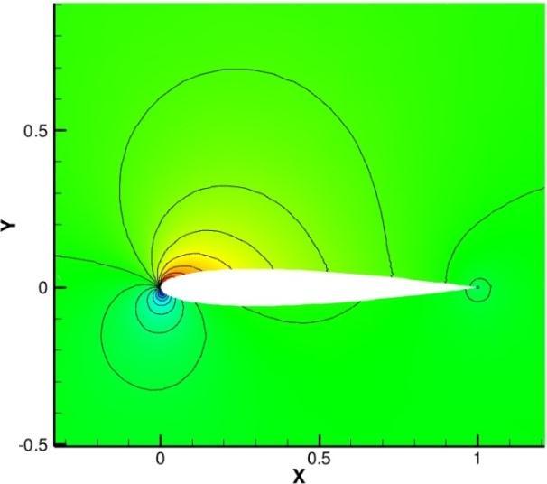
56 47 (d) Pressure Contour 3 rd order (e) Mach Number Contour 3 rd order Fgure 11. Mxed Mesh #2 and 4 th Order Results for Flow around a Cylnder. Fgure 12. The Mxed Grd n the Smulaton of Flow around NACA0012 Arfol.

57 48 (a) Pressure Contour (b) Mach Number Contour Fgure nd Order Soluton of the Flow around NACA0012 Arfol. (a) Pressure Contour (b) Mach Number Contour Fgure rd Order Soluton of the Flow around NACA0012 Arfol.

58 49 (a) Pressure Contour (b) Mach Number Contour Fgure th Order Soluton of the Flow around NACA0012 Arfol. Fgure 16. Entropy Error on the Upper Wall of NACA0012 Arfol.

59 50 CHAPTER 3. Dfferental Formulaton of Dscontnuous Galerkn and Related Methods for the Naver-Stokes Equatons A paper submtted to the Communcatons n Computatonal Physcs Hayang Gao, Z.J. Wang and H.T. Huynh Abstract A new approach to hgh-order accuracy for the numercal soluton of conservaton laws ntroduced by Huynh and extended to smplexes by Wang and Gao s renamed CPR (correcton procedure or collocaton penalty va reconstructon). The CPR approach employs the dfferental form of the equaton and accounts for the umps n flux values at the cell boundares by a correcton procedure. In addton to beng smple and economcal, t unfes several exstng methods ncludng dscontnuous Galerkn, staggered grd, spectral volume, and spectral dfference. To dscretze the dffuson terms, we use the BR2 (Bass and Rebay), nteror penalty, compact DG (CDG), and I-contnuous approaches. The frst three of these approaches, orgnally derved usng the ntegral formulaton, were recast here n the CPR framework, whereas the I-contnuous scheme, orgnally derved for a quadrlateral mesh, was extended to a trangular mesh. Fourer stablty and accuracy analyses for these schemes on quadrlateral and trangular meshes are carred out. Fnally, results for the Naver-Stokes equatons are shown to compare the varous schemes as well as to demonstrate the capablty of the CPR approach. 1. Introducton Second-order methods are currently popular n flud flow smulatons. For many mportant problems such as computatonal aeroacoustcs, vortex-domnant flows, and large eddy and drect numercal smulaton of turbulent flows, the number of grd ponts requred by a second-order scheme s often beyond the capacty of current computers. For these problems, hgh-order methods hold the promse of accurate solutons wth a manageable number of grd ponts. Numerous hgh-order methods have been developed n the last two decades. Here, we focus only on those that employ a polynomal to approxmate the soluton n each cell or element, and the polynomals collectvely form a functon whch s dscontnuous across cell boundares. Commonly used methods of ths type nclude

60 51 dscontnuous Galerkn (DG) [5-7,2,3], staggered-grd (SG) [15], spectral volume (SV) [24-28], and spectral dfference (SD) [17-19]. Among these, DG and SV are usually formulated va the ntegral form of the equaton, whereas SG and SD, the dfferental one. From an algorthm perspectve, the dfference among these methods les n the defnton of the degrees of freedom (DOFs), whch determne the polynomal n each cell, and how these DOFs are updated. Hgh-order methods for conservaton laws dscussed above deal wth the frst dervatve. Dffuson problems (vscous flows) nvolve the second dervatve. There are many ways to extend a method of estmatng the frst dervatve to the second; Arnold et al. analyzed several of them n [1]. Here, we restrct ourselves to approaches of compact stencl: the second dervatve estmate n an element nvolves data of only that element and the mmedate face neghbors. Such approaches have several advantages: the assocated boundary condtons are smpler, the codng s easer, and the mplct systems are smaller. The four schemes of compact stencl employed are BR2 (Bass and Rebay) [4], compact DG or CDG [20], nteror penalty [9,12], and I-contnuous (the value and dervatve are contnuous across the nterface) [14]. The BR2 scheme, an mprovement of the noncompact BR1 [2], s the frst successful approach of ths type for the Naver-Stokes equatons. The CDG scheme s a modfcaton of the local DG or LDG [8] to obtan compactness for an unstructured mesh. The nteror penalty scheme s employed here wth a penalty coeffcent usng correcton functon [14]. The I-contnuous approach s hghly accurate for lnear problems on a quadrlateral mesh. Ncknamed poor man s recovery, t can be consdered as an approxmaton to the recovery approach of Van Leer and Nomura [23]. (The recovery approach s beyond the scope of ths paper snce, although t s more accurate than the schemes dscussed here based on Fourer analyss [14], s more complex and costly.) For conservaton laws, Huynh (2007) [13] ntroduced an approach to hgh-order accuracy called flux reconstructon (FR). The approach solves the equatons n dfferental form. It evaluates the frst dervatve of a dscontnuous pecewse polynomal functon by employng the straghtforward dervatve estmate together wth a correcton whch accounts for the umps at the nterfaces. The FR framework unfes several exstng

61 52 methods: wth approprate correcton terms, t recovers DG, SG, SV, SD methods. Ths framework was extended to dffuson problems usng quadrlateral meshes n [14], where several exstng schemes for dffuson were recast and analyzed. Wang and Gao (2009) [29] extended the FR dea to 2D trangular and mxed meshes wth the lftng collocaton penalty (LCP) formulaton. The LCP methods was appled to solve the Euler and later Naver- Stokes equatons n both two [10] and three dmensons [11]. Due to ther tght connecton, the FR and LCP methods are renamed correcton procedures va reconstructon or CPR. The CPR formulaton does not nvolve numercal ntegratons; the mass matrx nverson s bult-n and therefore not needed; as a consequence, the approach s smpler and generally results n schemes more effcent than those by quadrature-based formulatons. In the present study, we demonstrate the capablty of the CPR formulaton for the numercal solutons of the Naver-Stokes equatons as well as nvestgate the performance of several dscretzaton approaches for dffuson. To accomplsh these obectves and to prepare for complex geometres and vscous boundary layers, we frst formulate the CPR framework on hybrd meshes of quadrlaterals and trangles. Next, we recast the four approaches for dffuson dscussed above n ths framework. Fourer stablty and accuracy analyses of these schemes are then carred out on square and trangular meshes. Fnally, results for several benchmark problems are shown. The paper s organzed as follows. The CPR formulaton for hybrd meshes s presented n secton 2. Secton 3 descrbes the dscretzaton of dffuson/vscous terms. Fourer analyses of the schemes for dffuson on square and trangular meshes are carred out n secton 4. Numercal tests are shown n Secton 5 for the Posson and the Naver-Stokes equatons. Conclusons are drawn n Secton Governng Equatons and Numercal Formulatons 2.1 Governng Equatons For the scalar case, we consder the heat equaton 2 ut u f (2.1) wth approprate boundary condtons. Our goal s to obtan numercal solutons for the Naver-Stokes equatons n conservatve form

62 53 Q F G 0 t x y (2.2) where Q s the vector of conserved varables, and F and G are the flux vectors formed by v v the nvcd and vscous parts, F F F, G G G. More precsely, u v 2 u p u uv Q, F, G 2, v uv p v E u E p ve p (2.3) and 0 2ux ux vy v F v, x u y C p u 2ux ux vy vvx uy T x Pr 0 vx u y v G 2v. y ux vy C p u vx uy v 2vy ux vy T y Pr (2.4) In (2.3)-(2.4), s densty, u and v velocty components n x and y drectons, p pressure, E total energy, dynamc vscosty, C specfc heat at constant pressure, Pr Prandtl p number, andt temperature. For a perfect gas, pressure s related to total energy by p 1 E u v (2.5) The rato of specfc heats s assumed to be constant, and γ=1.4 for ar. In addton, s set to -2/3 accordng to the Stokes hypothess.

63 54 From (2.4), the vscous fluxes can be wrtten as functons of both the conservatve varables and ther gradents, v v v v F F Q, Q, G G Q, Q. (2.6) v Note that the flux n the heat equaton s a specal case of the above:, v G Q, Q Q y. Therefore, from here on, we employ only (2.6). 2.2 CPR (Correcton Procedure va Reconstructon) Formulaton General CPR Formulaton F Q Q Q x and The CPR formulaton can be derved from a weghted resdual method by transformng the ntegral formulaton nto a dfferental one. Frst, a hyperbolc conservaton law can be wrtten as Q FQ ( ) 0, (2.7) t wth proper ntal and boundary condtons, where Q s the state vector and F ( F, G) s the flux vector. The computatonal doman s dscretzed nto N non-overlappng elements { V }. Let W be an arbtrary weghtng functon. The weghted resdual of Eq. (2.7) on element V can be wrtten as Q Q F( Q) WdV WdV WF( Q) nds W F( Q) dv 0. t t (2.8) V V V V Let Q be an approxmate soluton to Q at element. We assume that n each element, the k soluton belongs to the space of polynomals of degree k or less,.e., Q P V there s no confuson) wth no contnuty requrement across element nterfaces. The numercal soluton Q should satsfy Eq. (2.8),.e.,, (or k P f Q WdV WF ( Q ) nds W F ( Q ) dv 0. t (2.9) V V V

64 55 Snce the soluton s dscontnuous across element nterfaces, the above surface ntegral s not well-defned. To remedy ths problem, a common normal flux s employed: F( Q ) n F ( Q, Q, n), (2.10) n com where Q s the soluton on V, whch s outsde V. Instead of (2.9), the soluton s requred to satsfy Q WdV n WF com ds W F ( Q ) dv 0. t (2.11) V V V Applyng ntegraton by parts agan to the last term of the above LHS, we obtan Q WdV W F Q dv W F F Q ds n n ( ) com ( ) 0. t (2.12) V V V Here, we requre test space to have the same dmenson as the soluton space. The test space s chosen n a manner to guarantee the exstence and unqueness of the numercal soluton. Note that the quantty FQ ( ) nvolve no nfluence from the data n the neghborng cells; the nfluence of these data s represented by the above boundary ntegral, whch s also called a penalty term, penalzng the normal flux dfferences. The next step s crtcal n the elmnaton of the test functon. The boundary ntegral k above s cast as a volume ntegral va the ntroducton of a correcton feld P, n W dv W[ F ] ds, (2.13) V V n n n where [ F ] F ( Q, Q, n) F ( Q ) s the normal flux dfference. The above equaton s com sometmes referred to as the lftng operator, whch has the normal flux dfferences on the k boundary as nput and an element of (2.12), we obtan P V as output. Substtutng Eq. (2.13) nto Eq.

65 56 Q F( Q ) WdV 0. t (2.14) V k 1 If the flux vector s a lnear functon of the state varable, then F Q P. In ths case, the terms nsde the square bracket are all elements of P k. Because the test space s selected to ensure a unque soluton, Eq. (2.14) s equvalent to Q t FQ ( ) 0 (2.15) P V. As a k For non-lnear conservaton laws, FQ s usually not an element of k result, we approxmate t by ts proecton onto P V, denoted by to defne ths proecton s Eq. (2.14) then reduces to d F Q. One way F Q W V F Q WdV (2.16) V V Q t FQ ( ) 0. (2.17) Wth the ntroducton of the correcton feld, and a proecton of F Q for non-lnear conservaton laws, we have reduced the weghted resdual formulaton to a dfferental formulaton, whch nvolves no ntegrals. Note that for defned by (2.13), f W P k, Eq. (2.17) s equvalent to the DG formulaton; f W vares on another space, the resultng s dfferent, and we obtan a formulaton correspondng to a dfferent method [29]. Next, let the degrees-of-freedom (DOFs) be the solutons at a set of pontsr ( vares from 1 to K) called soluton ponts (SPs), as shown n Fgure 1. Then Eq. (2.17) holds true at the SPs,.e.,, Q t, FQ ( ) 0, (2.18),,

66 57 where F( Q, ) F( Q ). r, Along each edge, we also need to defne k+1 ponts where the common normal fluxes are calculated; these ponts are called flux ponts (Fgure 1). Once the soluton ponts and flux ponts are chosen, the correcton at the SPs can be wrtten as 1 [ F ] S, (2.19) n,, f, l f, l f V f V l where, f, l are constants ndependent of the soluton. Here, agan, s the ndex for soluton ponts on each cell, the cell ndex, f the face ndex, l the ndex of flux ponts on face f, and S f the area. Note that the correcton for each soluton pont, namely,, s a lnear combnaton of all the normal flux dfferences on all the faces of the cell. Conversely, a normal flux dfference at a flux pont on a face, say (f, l) results n a correcton at all soluton ponts of n an amount, f, l[ F ] f, l S f / V. n Along each edge f, the flux dfference values [ F ] f, lat the flux ponts defnes a 1-D polynomal of degree k denoted by F n f. Eq. (2.13) can then be wrtten as V fv n k, k. f f f W L dv W F ds (2.20) Here L s the Lagrange polynomals, and W k the test functons. Ths equaton yelds a lnear system as k vares; the unknowns are, ; both k and vary from 1 to K. By settng Wk Lk, the unknowns can be solved and the coeffcents can be determned. Note that after the approxmaton usng the Lagrange polynomals (1D and 2D), the volume and surface ntegrals are carred out exactly n (2.20) for the soluton of the lnear system. To compute the term, f, l F Q effcently, ether chan-rule or Lagrange polynomal approach can be used, detals about the two approaches can be found n Ref. [29].

67 58 Substtutng (2.19) nto (2.18) we obtan the followng correcton procedure va reconstructon (CPR) formulaton Q, 1 n F( Q, ), f, l[ F ] f, ls f 0 t. (2.21) V f V l It was shown that the locaton of SPs does not affect the numercal scheme for lnear conservaton laws [22, 13]. For effcency, therefore, the soluton ponts and flux ponts are always chosen to nclude corners of the cell; n addton, the soluton ponts are chosen to concde wth the flux ponts along cell faces. Furthermore, n a computaton wth hybrd mesh, the flux ponts are always of the same dstrbuton for dfferent cell types for ease of nterface treatment (Fgure 2). For the 2D cases presented here, the Legendre Lobatto ponts along the edges are used as the flux ponts and also (part of) the soluton ponts for both trangular and quadrlateral cells. CPR for 1D For the one-dmensonal (1D) case, consder the element V [ x 1/2, x 1/2 ] ; here, the flux F s F. Assumng a lnear flux for dervaton purpose, Eq. (2.21) takes the form Q FQ (,, ) n n, L[ F ] L, R[ F ] R 0, t x (2.22) n n where [ F ] and [ F ] L The quanttes L, and, R are the flux dfferences on the left and rght nterfaces of the cell V. R are the correcton coeffcents. Recall that for the 1D case, the number of soluton ponts s K=k+1; as a result, vares from 1 to K, and L, defne a polynomal of degree k=k 1 as vares. Ths polynomal s the dervatve of a correcton functon, whch approxmates the zero functon as explaned below. In 1D, the CPR method s equvalent to the flux reconstructon approach. The FR approach s a more general and flexble framework, makng t very easy to obtan varous sets of the coeffcents L,. The FR approach for both convecton and dffuson equatons s documented by Huynh n [13] and [14].

68 59 Therefore, we now dscuss (2.22) va the FR approach. Due to the dscontnuty at the nterfaces of the pecewse soluton polynomal, the flux s also a pecewse dscontnuous functon. The dea of the FR method s to construct a new flux functon F ˆ ( x ), whch satsfes the followng three crtera: Q ; F ˆ ( x ) s a degree k+1 polynomal,.e., one degree hgher than the soluton polynomal F ˆ ( x ) approxmates F (x) n some sense. In other words, some norm of the dfference Fˆ ( x) F ( x) s mnmzed; At both ends of the element, the flux takes on the value of the common fluxes,.e Fˆ ( x ) F ( Q ( x ), Q ( x )) F 1/2 com 1 1/2 1/2 com, 1/2 Fˆ ( x ) F ( Q ( x ), Q ( x )) F, 1/2 com 1/2 1 1/2 com, 1/2 where, at each nterface, F ( Q, Q ) com s a common nterface flux obtaned from the two values Q and Q to the left and rght of that nterface. For the nvscd flux, the Remann or upwnd flux s employed. For the dffuson or vscous flux, the common quanttes wll be dscusses n secton 4. Once ths flux functon F ˆ ( x ) s found, the DOFs are updated usng the followng dfferental equaton Q t F ˆ ( x ) x 0. (2.23),, Next, the reconstructed flux functon s re-wrtten as Fˆ ( x ) F ( x ) ( x ), (2.24) where (x) approxmates the zero functon. The functon (x) s further expressed as com, 1/2 1/2 L com, 1/2 1/2 R ( x) [ F F ( x )] g ( x) [ F F ( x )] g ( x), (2.25)

69 60 where g L (x) and g R (x) are called correcton functons. They are of degree k+1, approxmate the zero functon, and satsfy gl( x 1/2 ) 1, gl( x 1/2 ) 0 (2.26) g ( x ) 0, g ( x ) 1. - R 1/2 R 1/2 For g L, the condton g L (x 1/2 )=1 deals wth the ump at the left nterface, and the condton g L (x +1/2 )=0 leaves the rght nterface value unchanged. Eq. (2.22) then becomes Q, F ( x, ) [ Fcom, 1/2 F ( x 1/2 )] g L( x, ) [ Fcom, 1/2 F ( x 1/2 )] g R( x, ) 0. t x (2.27) Due to symmetry, we only need to consder g L (x), or smply g(x). Usng a lnear transformaton, t suffces to consder the correcton functon g on the standard element [ 1, 1].Snce g s a polynomal of degree k=k 1, t s defned by k+1 condtons. Two condtons are gven by the frst half of (2.26), namely g( 1) 1and g ( 1) 0. Thus, k 1 condtons reman. The requrement of approxmatng the zero functon can be satsfed by the k 2 condton that g s orthogonal to P,.e., k g( d 0, k 0,1,..., k 2 (2.28) Such a correcton functon s the Radau polynomal, and (2.22) results n a dfferental formulaton of the DG method. For other correcton functons, see [13, 14]. CPR for quadrlateral elements The 1D CPR formulaton can be extended to quadrlateral cells by tensor products. Frst, the mappng from the standard square [ 1,1]x[ 1,1] to a quadrlateral element (Fgure 3) s gven by x x, (2.29) N n M (, ) y 1 y where x and y are the physcal coordnates, ξ and η the local coordnates, (x, y ) are the control ponts of the mappng (the four corners for straght-edge elements). N n s the

70 61 number of nodes used to defne the physcal element, Nn 4 for elements wth straght edges, Nn 4 for elements wth one or more curved edges. For each, M (, ) s the shape functon, whch takes on the value 1 at node and 0 at all other nodes. The Jacoban of the formulaton s J ( xy, ) (, ) x y x y. (2.30) Assumng that the transformaton s nonsngular, the metrcs can be computed by x y / J, y x / J, x y / J, y x / J. (2.31) On the computatonal doman, the governng equaton takes the form Q F G 0, t (2.32) where Q J Q (2.33) F J( F G) (2.34) x y G J( F G). (2.35) x y Next, set S J( x, y), S J( x, y). Then we have F F S, G F S. In our mplementaton, J and S, S are stored at the soluton ponts. Wthn the th element, the soluton polynomal s a tensor product of 1D Lagrange polynomals,.e., k1 k1 Q (, ) Q L ( ) L ( ). (2.36) ;, m m m1 1

71 62 There are K=(k+1) 2 soluton ponts nsde each element. Here Q ;, m are the state varables at the soluton pont (,m) of cell, for clarty we use ; to separate the cell ndex from the two ndces,m of the soluton pont, wth the ndex n ξ drecton, and m, η drecton; L () and L ( ) are 1D Lagrange polynomals n ξ and η drectons, respectvely. The m fluxes F ;, m and G ;, m can be calculated by usng F( Q ;, m), G( Q ;, m). The fluxes can be represented wth Lagrange nterpolaton polynomals n the followng form: k1 k1 F (, ) F L ( ) L ( ), (2.37a) ;, m m m1 1 k1 k1 G (, ) G L ( ) L ( ). (2.37b) ;, m m m1 1 Common normal fluxes at the nterfaces are computed at all four element edges as follows: n Fcom ( 1, ) Fcom ( Q( 1, ), Q ( 1, ), n) S, (2.38a) n Fcom (1, ) Fcom ( Q(1, ), Q (1, ), n) S. (2.38b) The equatons for G s smlar. Fnally the DOFs are updated usng the followng equaton Q ;, m F (, m,, m) G (, m,, m) t [ F ( 1, ) F ( 1, )] g( ) [ F (1, ) F (1, )] g( ) com, m, m L, m com, m, m R, m [ G (, 1) G (, 1)] g( ) [ G (,1) G (,1)] g( ) 0. com, m, m L, m com, m, m R, m (2.39) Note that the correcton s done n a 1D manner. CPR for trangular elements, f, l The CPR method for trangular elements s computatonally effcent: the coeffcents are not only ndependent of the soluton, but also ndependent of the shape of the

72 63 element. Ths means once the dstrbuton of the soluton ponts s chosen, the coeffcents, f, l can be computed analytcally on a standard trangle by Eq. (2.20), and then appled to an arbtrary trangular element. The same comment holds for tetrahedral elements n 3D. The value of coeffcents for specfc sets of soluton ponts can be found n [29]. 3. Compact schemes for dscretzaton of the dffuson/vscous term 3.1 Basc Framework, f, l We now use the CPR formulaton dscussed above to dscretze the dffuson term. Ths dscretzaton ncludes two parts: calculate the dvergence of flux element and evaluate the common flux at the nterface. F on the nteror of the Frst, followng [2], we ntroduce a new varable R : R Q (3.1) Eq. (3.1) s solved usng the weak formulaton. In the CPR framework, the result s a collocaton formulaton: 1 com R Q [ Q Q ] n S, (3.2),, f, l f, l f f V f V l where Q s the common soluton on nterface f, and Q ;, com f, l com com face f. The defnton of Q Q Q, Q, n f l s the soluton wthn cell on vares wth dfferent approaches to dscretze the dffuson terms. Here, wth unquely defned left and rght sde for each nterface, Q and Q are the left and rght solutons, and n the unt normal from left to rght. Next, the vscous fluxes at soluton ponts are evaluated by,,, F F Q R G G Q R. (3.3) v v v v,,,,,, v v Then, F / xand G / ycan be obtaned (usng Lagrange polynomal). The dvergence of the flux namely F on the nteror of the element can be calculated.

73 64 Besdes those nteror dervatves, common dffuson/vscous fluxes at the nterfaces are also needed for the CPR formulaton v F F Q, Q, G G Q, Q. (3.4) com v com com com com com f, l f, l f, l f, l f, l f, l Ths means we also need to defne a common gradent Q Q Q Q Q Q n at the cell nterfaces. com com,,,, In the followng subsectons, we defne com Q and com Q by the BR2, I-contnuous, nteror penalty and CDG schemes. Let the face f be fxed. We focus our attenton on ths face and the cells on both sdes. 3.2 BR2 The common soluton n BR2 s smply the average of solutons at two sdes of the face For the common gradent, Q com f, l Qf, l Qf, l. (3.5) 2 com 1 Qf, l Qf, l rf, l Qf, l rf, l. (3.6) 2 where Q f, land Q f, lare the gradents of the soluton of the left and rght cells wth no correcton, whle r f, land r, soluton on only the face f. More precsely, f l are the correctons to the gradents due to the common the Nfp 1 com f, l l, m f, m f f V m1 r [ Q Q ] n S, Nfp 1 com f, l l, m[ ] f, m f f V m1 r Q Q n S (3.7) where Nfp s the number of soluton ponts on face f,, lm s the coeffcent of correcton due to face f. Note that the ndces l and m vary on the face f and, for our choce of soluton ponts, l, m, f, m, where the ndex for the soluton ponts corresponds to the ndex l for

74 65 the flux pont on the face f. For trangular elements,, fxed dstrbuton of flux ponts. lm are dentcal for any face f wth a For quadrlateral elements, because the tensor product s used, r f, land r, f l are thus computed n a 1D manner, whch means the penalty matrx lm, reduces to a dagonal matrx. Therefore, for a quadrlateral element, we only need to consder the coeffcent l, ls l V f. Next, denote by l the quantty l on the standard element [-1,1] X [1,1]. Then l g ' 1. Ths s also of the same form as the dffuson dscretzaton of the FR method [14]. However, for a general quadrlateral element, l needs to be transformed back to l n the physcal doman (x, y) before beng nserted to Eq. (3.7). Dependng on the drecton (ξ or η) we are dealng wth, l and l can be related by or g ' 1 l x y l x y g ' 1 l x y l x y. (3.8) Accordng to the Fourer analyss by Huynh [14], the dervatve of Legendre polynomal g ' 1 offers the best accuracy for the lnear dffuson equaton, and therefore g ' 1 LE (the value s kk ( 1) / 2 for degree k polynomal) s used n all the lnear dffuson numercal tests presented later. For the N-S equatons, however, a slghtly larger coeffcent k k 1 2 / 2 s used to stablze the scheme. The same coeffcent s also used n the other 3 dffuson schemes. 3.3 I-contnuous The I-contnuous approach n 1D was proposed by Huynh (2009) [14]. Its basc dea s: nstead of prescrbng a common soluton com Q at the nterfaces, LE com Q s an unknown to be solved by the condton that the corrected dervatves Q x C s contnuous across the nterface

75 66 f. Once we obtan Q com, the common dervatve one value at the nterface. Q x com s also defned, snce there s only In the 2D case, requrng the corrected gradent C Q to be contnuous at the nterfaces would gve us two condtons contnuty n x and y drectons. Snce we are only solvng one varable com Q, we requre contnuty only n the normal drecton. The corrected gradents on the left (-) and rght (+) can be expressed as S Q Q [ Q Q ] n, Nfp C f com f, l f, l f, m l, m V m1 S Q Q [ Q Q ] n. Nfp C f com f, l f, l f, m l, m V m1 (3.9) Then we requre the gradent to be contnuous n the normal drecton Substtutng n (3.9), we have C C Q n Q n. (3.10) S S Q S Q S Nfp Nfp l, m f l, m f com f, m l, m f f, m l, m f Qf, m Qf, l n Qf, l n m1 V V m1 V V (3.11) Eq. (3.11) represents a lnear system, from whch Q can be easly solved. Then, the com f, l common vscous flux com Q s obtaned by C Q n Q n or Q n Q n com C com f, l f, l Q com f, l t Qf, r t Qf, l t. 2 (3.12) Here t s the unt vector tangental to the face. The drecton of t makes no dfference provded that same t s used for both sdes. In the case that one or both sdes of the face s a l, ls f quadrlateral cell, we can use l n (3.11). V Whle the I-contnuous approach s more nvolved than the other three schemes, t was shown n [14] va Fourer analyss that f g Le s employed as the correcton functon, there s

76 67 a sgnfcant gan n accuracy. Snce such a Legendre-polynomal correcton functon s not yet known on trangles, we use the equvalence of the Radau polynomal. Note that we need to solve a k+1 lnear system for each face. The cost of ths step s mnmal snce the matrces are ndependent of the soluton. They only need to be nverted once durng ntalzaton. Therefore, the I-contnuous approach s only slghtly costler than the BR2 approach. 3.4 Interor Penalty Interor penalty s a smplfed verson of BR2 for trangular meshes, and s dentcal to BR2 for quadrlateral meshes. In BR2 the correcton (or penalty) r f, land r, f l at one face flux pont s a lnear combnaton of the soluton dfferences of all ponts on the face. In nteror penalty method, the penalty s only dependent on the soluton dfference at that pont,.e. the penalty s computed n a 1-D manner. Therefore, equatons (3.5) and (3.6) stll holds for nteror penalty method, the only dfference les n the computaton of the correctons due to the common soluton, S com f S com f rf, l Q Q g ' 1 n, r, ' 1, f, l f l Q Q g n V f, l V (3.13) S f V n here s n the place of terms lke x, y the length scale factor. 3.5 CDG for the quadrlateral mesh, whch represents The dea of CDG s to use one sde of the face for the common soluton and the other sde for the common gradent. For example, f we use the rght (+) sde for common soluton and the left (-) sde for common gradent, we obtan, where Q com f, l Q f, l (3.14) Q Q r, (3.15) com f, l f, l f, l fp 1 N com f, l l, m f, m f f V m1 r Q Q n S (3.16)

77 68 Alternatvely, we can also use the opposte sdes for common soluton and common gradent. Note that the dfference between the CDG and LDG methods s n the defnton of the common gradent. At a fxed face, for CDG, the correcton term r f, l n 3.16 nvolves only the umps at that face, whereas, for LDG, t nvolves the umps at all the faces of the correspondng cell. 3.6 Boundary Condtons In ths subsecton, we dscuss the boundary condtons for the compact dffuson/vscous schemes. Let s assume a face f s on the boundary of the computatonal doman and the left sde of f s the computatonal doman. Only the solutons and gradents on the left (-) sde are avalable, and the fnal obectve s to obtan com Q and com Q for face f. In the lnear dffuson cases presented n Secton 5, two types of boundary condtons are used. For Drchlet boundary condton, Q s set to the boundary value whle the gradent s extrapolated,.e. Q Q. Then the common quanttes can be computed accordng to Secton For Neumann boundary condtons, the common soluton s extrapolated com Q Q, whle com Q s set to the boundary value. In the case of Naver-Stokes equatons, the boundary condton s smlar to the Drchlet boundary condton for the lnear case. Q can be smply fxed to the exact boundary values, or obtaned through characterstc boundary condtons. For sold nonslppng walls, Q s set to Q wth reversed velocty, resultng zero velocty for com Q. The gradents are always extrapolated from the nteror doman,.e. Q Q. For adabatc walls, the normal temperature gradents are set to 0 when computng the fluxes by Equaton (3.4). 4. Two-Dmensonal Fourer (Von Neumann) Analyss We now carry out the Fourer (Von Neumann) stablty and accuracy analyss of the schemes dscussed above on a square and a trangular mesh. On the doman (, ) (, ), consder the dffuson equaton ut uxx u (4.1) yy

78 69 Wth ntal condton u nt ( x) I ( wx xwy y) e, where and I 1 (we use for the cell ndex), and the wave numbers w x and w y le between and. Low frequency data corresponds to wave numbers of small magntude; hgh frequency, to those near. The exact soluton s u exact ( x) ( 2 2 wx wy ) t I ( wx xwy y) e e. At ( x, y, t) (0,0,0), 2 2 ( uexact ) t (0,0,0) ( wx wy ). (4.2) Square-Mesh Case. The cells are [, 1] [, 1]. Assume the soluton s represented E, by degree k polynomal. The soluton ponts on each square are formed by usng tensor product; thus, there are K k 1 2 of them. Denote by u, the column vector of K soluton values u ( u, u,..., u, u,..., u,..., u,..., u ) T,,, 1,1,, 1,2,, 1, k1,, 2,1,, 2, k1,, k1,1,, k1, k1 (4.3) where the superscrpt T denotes the transpose. The followng property of the data plays a key role n the calculaton of egenvalues, Iw Iw x y 1, e, and, 1 e, u u u u (4.4) For the schemes of compact stencl dscussed here, the soluton can be expressed as where all du dt, C u C u C u C u C u (4.5) 0,0, 1,0 1, 1,0 1, 0, 1, 1 0,1, 1 Iw C, are K K matrces. Usng (4.4), we replace u 1, by e x u,, and smlarly for all terms of the rght hand sde above. The result s where du dt, Su (4.6) Iwx Iw Iwy Iw x y 0, 0 e 1, 0 e 1, 0 e 0, 1 e 0,1, S C C C C C. (4.7) Here, S, whch stands for space or semdscrete, s a K K matrx wth K egenvalues. 2 2 The one approxmatng ( w ) s called the prncpal egenvalue and s denoted by S w x, w ) : ( y x w y S( w, w x y 2 x 2 y ) ( w w ). (4.8)

79 70 All other egenvalues are spurous. For stablty, all egenvalues must have nonpostve real parts. It turns out that for all methods dscussed, va Fourer analyss, the scheme on a square mesh and the correspondng 1D verson have the same order of accuracy. Concernng stablty (tme-steppng) lmts, the method on a square mesh has a lmt of 1/2 that of the 1D verson. That s, the largest magntude of all egenvalues n the case of a square mesh s twce that of the correspondng 1D method. Ths reducton by a factor of 2 n the stablty lmt for the 2D dffuson equaton s consstent wth the reducton by a factor of 2 for advecton equaton n [13,14]: each dervatve corresponds to a reducton by 2. The mnmum egenvalues, orders of accuracy, and errors of the schemes on a square mesh are shown n Table 1. In the calculatons of order of accuracy, the coarse mesh corresponds to w and w 10, and the fne mesh, w 16 and w 20. Next, x y 2 2 the prncple egenvalue S wx, wy s compared to the exact egenvalue wx wy x y to determne the error of the scheme. The errors E(w) and E(w/2) are then evaluated for the wave numbers of the coarse and fne meshes respectvely. The order of accuracy s E w calculated by Log Log 2 2 [14]. E w/2 Note that all schemes are of order at least 2k,.e., they are super-convergent for k 2. The advantage of the CDG scheme s that ts accuracy order s 2k 1 ; ts dsadvantage s that the mnmum egenvalues have rather large magntudes (nearly three tmes) compared to those of the other schemes. Also note that for the square mesh case, the nteror penalty (IP) scheme reduces to the BR2 scheme. As for the I-contnuous scheme, the one employed here s the member whose trangular-mesh verson s readly avalable,.e., the member usng the correcton functon g DG not the most accurate member, whch employs the Legendre polynomal as correcton functon. Compared to BR2, the I-contnuous scheme has a smaller error as well as a mnmum egenvalue wth a smaller magntude. Trangular-Mesh Case. Each square E, [, 1] [, 1] s cut nto two trangles by the dagonal from the northwest to the southeast corners. To carry out the Fourer analyss

80 71 for the trangular-mesh case, we must par up these two trangles so that the soluton vector on each square has a repeatable pattern explaned below. Recall that f k s the degree of polynomal representng the soluton, then the correspondng number of soluton ponts on each trangle s K k 2 ( k 1) / 2. Combnng the data on two trangles, denote the vector of 2K entres on the square E, by, u. The data u, s repeatable n the sense that (4.4) holds. The semdscrete equaton s smlar to (4.5) and, the correspondng 2K 2 matrx S, (4.7). The mnmum egenvalues, orders of accuracy, and errors of the schemes on a trangular mesh are shown n Table 2. In the order of accuracy calculatons, agan, the coarse mesh corresponds to w and w 10, and the fne mesh, w 16 and w 20. x y Note that all schemes are of order 2k. For a trangular mesh, the CDG scheme s no longer of order 2k 1.It has the same order of accuracy as the other schemes, but ts error s consderably smaller than those of the others. The dsadvantage of the CDG scheme s that the mnmum egenvalues have rather large magntudes (roughly three tmes) compared to those of the other schemes. Compared to BR2, the I-contnuous scheme s slghtly less accurate n ths case; however, t has the advantage that ts mnmum egenvalue has a slghtly smaller magntude. Comparng Table 2 to 1,.e., the schemes on a trangular mesh verses those on a square mesh, accuracy on a trangular mesh s better, but stablty lmt s worse. The reason s perhaps that correspondng to each k, there are more soluton ponts on (the two trangles of ) the square n the former case compared to the latter (.e., k2k 1 versus k 1 2 ). As the last remark of ths secton, note that n practce, when the mesh s non-unform and the equatons are nonlnear, the super-accuracy (or super-convergence) property no longer holds. In fact, even for the case of a unform mesh and lnear equatons, snce the data s approxmated by a polynomal of degree k n each cell, f we smply compare the numercal soluton wth the exact one, the degree of accuracy s only k 1 ; to observe super-accuracy, we may need to compare specal quanttes such as the average of the x y

81 72 solutons on each square (even when the mesh s trangular). In short, super accuracy results do not hold n practce. 5. Numercal Results 5.1 Posson s Equaton The followng Posson s equaton u xx 2 x y uyy sn sn 2 2 2, (5.1) x y wth the exact soluton u sn sn s solved on the doman [0, 1]X[0, 1] wth 2 2 both regular quadrlateral meshes and rregular trangular meshes (Fgure 4). The soluton varable u s fxed to the exact soluton at the boundary faces. The CPR solver starts wth the exact soluton and marches forward n tme wth an LUSGS tme ntegraton [21] untl the resdual reaches machne zero. The L 2 norm of the errors at the soluton ponts s evaluated and the order of accuracy s calculated va an h-refnement by p ln Er / Er 1 2 (5.2) ln N / N 2 1 where Er and 1 Er are the error norms for mesh 1 and mesh 2, wth number of cells N 2 1 and N 2 respectvely. (The error s always calculated n ths manner n the rest of the paper). Table 3 shows the accuracy results of the BR2, I-contnuous and CDG approaches on quadrlateral meshes. All schemes produce comparable errors and orders of accuracy, wth CDG bested the other two by a small margn.. Table 4 shows accuracy results for rregular trangular meshes. Agan, the errors by BR2, I-contnuous and nteror penalty schemes are comparable, and the CDG error s the best by a small margn 5.2 The Potental Flow over a Cylnder The potental for an ncompressble, rrotatonal and nvscd flow satsfes the Laplace equaton (2.1). To test the CPR dffuson solver on curved boundares, the potental flow

82 73 over a cylnder wth radus r=1 s computed. The exact soluton for ths case s 1 exact x x y The soluton varable at the outer boundary faces s fxed to the exact soluton. For the nner boundary, the Neumann condton n 0 s mposed. The curved boundary s always represented by polynomals of the same degree as that of the soluton polynomals. The ntal condton s set to the exact soluton and an LUSGS solver s used wth a convergence crtera of machne zero for all cases. Fgure 5a shows the 10x10 structured quadrlateral O-mesh used n ths test case. Fgure 5b shows the 10x10x2 trangular mesh, whch s obtaned by cut each quadrlateral cell nto two trangles. Fgure 6 shows the soluton by the BR2 method wth p=2. Tables 5 and 6 respectvely show the numercal results for quadrlateral and trangular meshes. The L 2 errors produced by all the schemes seem comparable, and so s the order of accuracy. Fgure 7 shows the convergence hstory of the four schemes for p=3 on both quadrlateral and trangular meshes. The resduals are plotted aganst the teratons. Snce the cost per teraton of the four approaches s about the same, these fgures also represent the CPU tme used. For both quadrlateral and trangular meshes, BR2 and nteror penalty converge fastest and CDG, slowest. 5.3 The Couette Flow Compressble Couette flow between two parallel walls s used to evaluate the accuracy of the method on rregular mxed grds. The exact soluton for ths case s U u y, v 0 H p p Const,. (5.3) RT 2 y U y y T T T T H 2k H H

83 74 The followng parameters are chosen: the speed of the upper wall U=0.3, the temperature of the lower wall T 0 =0.8, the temperature of the upper wall T 1 =0.85, vscosty µ=0.01, doman heght (n y drecton) H=2, and the computatonal doman s a 4X2 rectangle. The flow varables at boundary faces are fxed to the exact soluton. All the tests cases presented below are obtaned wth an LUSGS mplct tme ntegraton approach [21], and all cases converge to machne zero. Densty errors are used for accuracy evaluaton. Fgure 8 shows the three meshes used n the mesh refnement study. The meshes are generated ndependently, rather than n an h-refnement manner. The schemes employed are 2 nd -4 th order accurate. The order of accuracy s also calculated by agan Equaton (5.2). Table 7 shows accuracy results for the four schemes. Agan, all the schemes are of comparable accuracy except for the case p=2 for CDG, where the order of accuracy s not qute as hgh as the others. The accuracy of CDG demonstrated n Fourer analyss and lnear dffuson case s not carred over to ths Naver-Stokes case. The BR2 and I- contnuous approaches perform consstently well, whereas the nteror penalty approach produces slghtly larger errors for the case p=1. Note that although the orders of accuracy of all the schemes are slghtly less than optmal, these results are obtaned wth hghly rregular and mxed meshes of poor qualty. 5.4 Lamnar Flow around a NACA0012 Arfol Vscous lamnar flow around a NACA 0012 arfol s smulated wth the CPR method, usng the BR2, I-contnuous, nteror penalty and CDG schemes for the vscous flux. 2 nd -5 th order schemes are tested. The flow condtons are Mach = 0.5 and Re = 5000, wth an angle of attack of 1 degree. Under such condtons, steady lamnar separatons are expected for both upper and lower surfaces of the arfol. Adabatc no-slp wall condton s prescrbed at the arfol surface. Subsonc characterstc far feld condton s used at the outer surface of the computatonal doman. The curved wall boundary s represented by the same degree polynomal as the soluton. The computatonal doman extends 20 chord lengths away from the center of the arfol. Fgure 9 shows the mesh of 2692 cells, whch s composed of regular quadrlateral elements near the arfol and rregular mxed elements elsewhere, wth some refnement at

84 75 the tralng edge. A LUSGS solver s used for tme ntegraton and all cases converge to machne zero. Fgure 10 (a-c) shows the computed Mach number contours of 2 nd 4 th order schemes. Only the BR2 results are shown, snce the results of other schemes are very smlar. Due to the coarse mesh, the 2 nd order results are not smooth, especally at the wake. Note that for the 3 rd and 4 th order cases, the contour lnes are smooth across the nterfaces between regular cells and rregular ones and also between trangular cells and quadrlateral ones. Vsually, 3 rd and 4 th order results are nearly dentcal. The skn frcton coeffcent C f s defned as C f w (5.4) 1 2 U 2 where the shear stress at wall s computed by same as u n. w V n, wth ts sgn chosen to be the Fgure 11 shows the C f dstrbuton near the separaton pont. For the four dffuson schemes, the 3 rd and 4 th order results are very close; ths fact ndcates convergence wth p- refnement. Except for the 2 nd dstrbutons of C f. order case, the four schemes produce almost dentcal Tables 8-10 show the computed pressure drag coeffcents C D,p, frcton drag coeffcents C D,f, and the separaton ponts on the upper wall. The data converge as the polynomal degree ncreases and, agan, there s no sgnfcant dfference among the four schemes consdered. Fgures 12(a, b) show the convergence hstory of the 4 th order case, whch provdes an estmate of the effcency of the four dffuson schemes. The same tme step, whch s also the largest allowable by stablty, s used for all schemes. In terms of both teraton and CPU tme, CDG s least effcent, whle the other three approaches show no sgnfcant dfference.

85 Unsteady Flow around a Crcular Cylnder The unsteady lamnar flow around a cylnder s smulated wth the 2 nd 4 th order CPR methods usng the BR2 dffuson scheme. The Reynolds number Re = 75, the free stream Mach number M = 0.2. A vortex street s expected to form n the wake of the cylnder. The frequency of the vortex sheddng s often called the Strouhal number defned by fl St. (5.5) s c U The length scale L c here s the dameter of the cylnder. In an expermental study by Wllamson [30], St was found to be Subsonc far feld boundary condton s used at the outer boundary of the doman. Adabatc wall condton s used for the cylnder surface. A 2 nd order unsteady LUSGS solver s used for tme ntegraton. Fgure 13 shows the mesh, whch contans 2,028 cells, wth regular quadrlateral cells near the cylnder and n the wake regon, and rregular mxed cells elsewhere. The effects of doman sze, tme step and convergence crtera of nner teratons are carefully studed to make sure the correct numercal soluton s obtaned. Fgure 14 (a-c) shows the nstantaneous Mach number contours. Note that the 2 nd order contours n (a) are not smooth. The 3 rd and 4 th order results are smooth and smlar, wth 4 th order contours smoother at 20 dameters downstream. Table 11 shows the average drag coeffcent CD and computed St for p=1-3. Both converge as p ncreases, and the computed St s comparable to the expermental data. 6. Conclusons The CPR formulaton, whch has the advantage of smplcty and economy, s extended to the dffuson and Naver-stokes equatons on hybrd meshes of trangles and quadrlaterals. The four schemes of compact stencl employed to dscretze the dffuson terms are BR2, nteror penalty, compact DG (CDG), and I-contnuous. The frst three of these schemes, orgnally derved usng the ntegral formulaton, were recast here n the CPR framework, whereas the I-contnuous scheme, orgnally derved for a quadrlateral mesh, was extended to a trangular mesh. Fourer stablty and accuracy analyses on

86 77 quadrlateral and trangular meshes were carred out. Numercal tests varyng from lnear dffuson to steady and unsteady lamnar flows were conducted. The results show that the CPR approach produces hghly accurate schemes of expected order of accuracy,.e., schemes usng polynomal of degree k s accurate to order k+1. Concernng methods for dffuson, the four compact schemes are comparable n terms of accuracy. In terms of convergence rate, however, the CDG scheme s slowest: ths fndng by numercal experments s consstent wth the fndng va Fourer analyss. Among the four schemes, due to ts smplcty, BR2 s an optmal choce; whle I-contnuous approach s promsng, a more accurate trangular-mesh verson must be found for the scheme to be compettve; the nteror penalty approach s the smplest, but s also slghtly less accurate. Fnally, the CPR formulaton presented here can be extended to 3D and, due to ts hybrdmesh capablty, the resultng methods can be appled to practcal problems nvolvng complex geometres. Acknowledgments The frst two authors were funded by AFOSR grant FA The thrd author s supported by NASA s Fundamental Aeronautcs Program. The vews and conclusons contaned heren are those of the authors and should not be nterpreted as necessarly representng the offcal polces or endorsements, ether expressed or mpled, of AFOSR, NASA or the U.S. Government. References [1] D.N. Arnold, F. Brezz, B. Cockburn and L.D. Marn, Unfed analyss of dscontnuous Galerkn methods for ellptc problems, SIAM J. Numer. Anal., 19(4): , [2] F. Bass and S. Rebay, A hgh-order accurate dscontnuous fnte element method for the numercal soluton of the compressble Naver Stokes equatons. J Comp Phys 1997;131(1): [3] F. Bass and S. Rebay, Hgh-order accurate dscontnuous fnte element soluton of the 2D Euler equatons, J. Comput. Phys. 138, (1997). [4] F.Bass and S. Rebay, GMRES Dscontnuous Galerkn Soluton of the Compressble Naver-Stokes Equatons. In Karnadaks Cockburn and Shu, edtors, 208. Sprnger, Berln, [5] B. Cockburn and C.-W. Shu, TVB Runge-Kutta local proecton dscontnuous Galerkn fnte element method for conservaton laws II: general framework, Mathematcs of Computaton 52, (1989). [6] B. Cockburn, S.-Y. Ln and C.-W. Shu, TVB Runge-Kutta local proecton dscontnuous Galerkn fnte element method for conservaton laws III: one-dmensonal systems, J. Comput. Phys. 84, (1989).

87 78 [7] B. Cockburn and C.-W. Shu, The Runge-Kutta dscontnuous Garlerkn method for conservaton laws V: multdmensonal systems, J. Comput. Phys., 141, , (1998). [8] B. Cockburn and C.-W. Shu, The local dscontnuous Galerkn methods for tme-dependent convecton dffuson systems, SIAM J. Numer. Anal., 35(1998), pp [9] V. Doleší, On the dscontnuous Galerkn method for numercal soluton of the Naver-Stokes equatons, Int. J. Numer. Methods Fluds, 45: , [10] H. Gao and Z.J. Wang, A Hgh-Order Lftng Collocaton Penalty Formulaton for the Naver-Stokes Equatons on 2-D Mxed Grds, AIAA [11] T. Haga, H. Gao and Z.J. Wang, A Hgh-Order Unfyng Dscontnuous Formulaton for 3-D Mxed Grds, AIAA [12] R. Hartmann and P. Houston, Symmetrc nteror penalty DG methods for the ncompressble Naver- Stokes Equatons I: Method formulaton. Int. J. Numer. Anal. Model., 1:1-20. [13] H.T. Huynh, A flux reconstructon approach to hgh-order schemes ncludng dscontnuous Galerkn methods, AIAA Paper [14] H.T. Huynh, A Reconstructon Approach to Hgh-Order Schemes Includng Dscontnuous Galerkn for Dffuson, AIAA Paper [15] D.A. Koprva and J.H. Kolas, A conservatve staggered-grd Chebyshev multdoman method for compressble flows, J. Comp. Physcs, 125(1996), pp [16] C. Lang, A. Jameson and Z. J. Wang, Spectral Dfference method for two-dmensonal compressble flow on unstructured grds wth mxed elements, Journal of Computatonal Physcs, vol 228, pp , [17] Y. Lu, Vnokur M, and Wang ZJ. "Dscontnuous Spectral Dfference Method for Conservaton Laws on Unstructured Grds," n Proceedngs of the 3rd Internatonal Conference on Computatonal Flud Dynamcs, Toronto, Canada, July [18] Y. Lu, Vnokur M, and Wang ZJ. "Dscontnuous Spectral Dfference Method for Conservaton Laws on Unstructured Grds," Journal of Computatonal Physcs Vol. 216, pp (2006). [19] G. May and A. Jameson, A spectral dfference method for the Euler and Naver-Stokes equatons, AIAA paper No , [20] J. Perare and P.-O. Persson, The compact dscontnuous Galerkn (CDG) method for ellptc problems, SIAM J. Sc. Comput., Vol. 30, No. 4 (2008) pp [21] Y. Sun, Z.J. Wang, and Y. Lu, Effcent mplct non-lnear LU-SGS approach for compressble flow computaton usng hgh-order spectral dfference method, Commun. Comput. Phys. Vol. 5, No. 2-4, pp [22] K. Van den Abeele, C. Lacor, and Z. J. Wang. On the stablty and accuracy of the spectral dfference method. J. Sc. Comput., 37(2): , [23] B. van Leer and S. Nomura, Dscontnuous Galerkn for Dffuson, AIAA Paper

88 79 [24] Z.J. Wang, Spectral (Fnte) volume method for conservaton laws on unstructured grds: basc formulaton, J. Comput. Phys. Vol. 178, pp , [25] Z.J. Wang, Hgh-order methods for the Euler and Naver-Stokes equatons on unstructured grds, Journal of Progress n Aerospace Scences, Vol. 43, pp. 1-47, [26] Z.J. Wang and Y. Lu, Spectral (fnte) volume method for conservaton laws on unstructured grds : one-dmensonal systems and partton optmzaton, Journal of Scentfc Computng, Vol. 20, No. 1, pp (2004). [27] Z.J. Wang and Y. Lu, Spectral (fnte) volume method for conservaton laws on unstructured grds : one-dmensonal systems and partton optmzaton, Journal of Scentfc Computng, Vol. 20, No. 1, pp (2004). [28] Z.J. Wang, L. Zhang and Y. Lu, Spectral (Fnte) Volume Method for Conservaton Laws on Unstructured Grds IV: Extenson to Two-Dmensonal Euler Equatons, Journal of Computatonal Physcs Vol. 194, No. 2, pp (2004). [29] Z.J. Wang and H. Gao, A unfyng lftng collocaton penalty formulaton ncludng the dscontnuous Galerkn, spectral volume/dfference methods for conservaton laws on mxed grds, Journal of Computatonal Physcs 228 (2009) [30] C. H. K. Wllamson. Oblque and parallel modes of vortex sheddng n the wake of a cylnder at low Reynolds number, J. Flud Mech., 206: , 1989.

89 80 Table 1. Mnmum egenvalues, orders of accuracy, and errors for schemes on a square mesh. Square-mesh case K 2 Mn. Egval. Ord. Acc. Coarse mesh error, w /8, w / 10 x y Fne mesh error, w /16, w / BR e e I-Contnuous e e IP = BR2 4. CDG e e-07 x y K 3 1. BR e e I-Contnuous e e IP = BR2 4. CDG e e-11 K 4 1. BR e e I-Contnuous e e IP = BR2 4. CDG e e-15

90 81 Table 2. Mnmum egenvalues, orders of accuracy, and errors for schemes on a trangular Trangular-mesh case K 2 Mn. Egval. Ord. Acc. mesh. Coarse mesh error, w /8, w / 10 x y Fne mesh error, w /16, w / BR e e I-Contnuous e e IP e e CDG e e-05 x y K 3 1. BR e e I-Contnuous e e IP e e CDG e e-10 K 4 1. BR e e I-Contnuous e e IP e e CDG e e-13 Table 3. Accuracy results of Posson s equaton wth regular quadrlateral mesh (Interor Polynomal Degree Penalty s dentcal to BR2). Mesh BR2 I-Contnuous CDG L2 error L2 order L2 error L2 Order L2 error L2 Order P=2 5x e e e-04-10x e e e x e e e x e e e P=3 5x e e e-06-10x e e e x e e e x e e e P=4 5x e e e-08-10x e e e x e e e

91 82 Table 4. Accuracy results of Posson s equaton wth rregular trangular mesh. Polynomal Degree P=2 P=3 Polynomal Degree P=2 P=3 # of BR-2 I-contnuous cells L2 error L2 order L2 error L2 order e e e e e e e e e e e e # of Interor Penalty CDG cells L2 error L2 order L2 error L2 order e e e e e e e e e e e e Table 5. Accuracy results for a potental flow over a cylnder wth quadrlateral meshes Polynomal Degree P=2 (Interor Penalty s dentcal to BR2). Mesh BR2 I-contnuous CDG L 2 error L 2 order L 2 error L 2 Order L 2 error L 2 Order 5x e e e-03-10x e e e x e e e P=3 P=4 5x e e e-04-10x e e e x e e e x e e e-05-10x e e e x e e e

92 83 Table 6. Accuracy results for a potental flow over a cylnder wth trangular meshes. Polynomal Degree P=2 P=3 Polynomal Degree P=2 P=3 Mesh BR-2 I-contnuous L 2 error L 2 order L 2 error L 2 order 10x10x e e-04-20x20x e e x40x e e x10x e e-05-20x20x e e x40x e e Mesh Interor Penalty CDG L2 error L2 order L2 error L2 order 10x10x e e-04-20x20x e e x40x e e x10x e e-05-20x20x e e x40x e e

93 84 Table 7. Accuracy results of Couette flow wth hybrd mesh. Polynomal Degree & BR2 I-contnuous Mesh (No. of cells) L 2 Error L 2 Order L 2 Error L 2 Order e e-05 - p= e e e e p= e e e e e e e e-09 - p= e e e e Polynomal Degree & Interor Penalty CDG Mesh (No. of L 2 Error L 2 Order L 2 Error L 2 Order p=1 cells) e e e e e e p=2 p= e e e e e e e e e e e e Table 8. Flow over a NACA0012 arfol pressure drag coeffcents CD,p BR2 I-Contnuous Interor Penalty CDG p= p= p= p= Table 9. Flow over a NACA0012 arfol frcton drag coeffcents CD,f BR2 I-Contnuous Interor Penalty CDG p= p= p= p=

94 85 Table 10. Flow over a NACA0012 arfol separaton pont on the upper surface. BR2 I-Contnuous Interor Penalty CDG p= % 78.30% 79.84% 80.39% p= % 68.65% 68.67% 68.67% p= % 67.81% 67.84% 67.82% p= % 67.90% 67.91% 67.91% Table 11. P-refnement study for unsteady flow around a cylnder. Vscous Method -- Polynomal Degree C D BR BR BR St

95 86 ˆ ] [ F f,3 ˆ ] [ F f,2 ˆ ] [ F f,1 Fgure 1. Soluton ponts (squares) and flux ponts (crcles) for k = 2. ˆ ] [ F f,3 ˆ ] [ F f,2 ˆ ] [ F f,1 Fgure 2. Soluton ponts for the 3rd order CPR scheme on hybrd meshes. (1, 1) (-1, -1) Fgure 3. Transformaton of a quadrlateral element to a standard element.

96 87 Fgure 4. Irregular trangular mesh for Posson s equaton on [0,1] X[0,1]. (a) Quadrlateral mesh (b) Trangular mesh Fgure 5. Meshes for potental flow over a cylnder.

97 88 Fgure 6. Soluton contours for potental flow over a cylnder (BR2, 3rd order, 20X20 mesh). (a) (b) Fgure 7. Convergence hstory of potental flow over a cylnder (4th order, 40x40 meshes) (a) quadrlateral mesh (b) trangular mesh.

98 89 (a) (b) (c) Fgure 8. Mxed mesh used for Couette flow (a) 10X5 wth 61 cells (b) 20X10 wth 250 cells (c) 40X20 wth 919 cells. Fgure 9. Mxed mesh around an NACA0012 arfol.

99 90 (a) 2 nd Order (b) 3 rd Order (c) 4 th Order Fgure 10. Mach number contours of flow around an NACA 0012 arfol.

100 91 Fgure 11. C f on the upper surface of NACA0012 arfol for BR2, I-contnuous, nteror penalty and CDG. (a) (b) Fgure 12. 4th order convergence hstory of lamnar flow over NACA0012 arfol n terms of (a) teratons (b) CPU tme.

101 92 (a) The whole doman (b) near the cylnder Fgure 13. Mxed mesh for unsteady flow around a cylnder. (a) 2 nd order (b) 3 rd order

102 93 (c) 4 th order Fgure 14. Mach number contours for unsteady flow around a cylnder.

103 94 CHAPTER 4. A Study of Curved Boundary Representatons for 2D Hgh-order Euler Solvers A paper publshed n the Journal of Scentfc Computng Hayang Gao, Z.J. Wang and Yen Lu Abstract The present study dscusses several approaches of representng curve boundares wth hgh-order Euler solvers. The am s to mnmze the soluton entropy error. The tradtonal boundary representaton based on nterpolaton polynomals s presented frst. A new boundary representaton based on the Bezer curve s then developed and analyzed. Several numercal tests are conducted to compare both representatons. The new approach s shown to have several advantages for complcated geometres. 1. Introducton The last two decades has wtnessed the emergence of several hgh-order methods, such as the dscontnuous Galerkn (DG) [1-4], spectral volume (SV) [10-12], spectral dfference (SD) [11,15], and the recently developed flux reconstructon (FR) [8] and lftng collocaton penalty (LCP) methods [16]. All the above methods use pecewse polynomals to approxmate the soluton wthn an element, and thus result n compact spatal dscretzatons. As hgh-order methods become ncreasngly mature for real world applcatons, the hghorder boundary treatment becomes a crtcal ssue. In manstream fnte volume solvers, the wall boundary of the geometry s usually represented by pecewse straght segments or planar facets. However, ths lnear boundary representaton s far from suffcent for hghorder methods. When the error from the geometry domnates the dscretzaton error, the beneft of hgh-order methods s largely lost. Thus, the curvlnear element was ntroduced by Gordon and Hall [6, 7] to solve the problem, whch was also used by Koprva [9] n the staggered-grd method. Bass and Rebay [1, 2] also dentfed the mportance of geometry representaton whle solvng the Euler equatons wth the DG method, and they demonstrated that hgh order boundary was mandatory f any meanngful soluton was to be

104 95 obtaned. Besdes, the order of boundary representaton should be as hgh as the order of the soluton reconstructon to acheve an optmal rate of convergence [1]. When developng the SV method for the Euler equatons, Wang and Lu [14] also addressed the mportance of hgh order boundary representaton. In ther numercal tests, t was found that hgher than quadratc boundary representaton s necessary to obtan any physcally acceptable solutons. In the above mplementatons of hgh order boundary, a polynomal geometrc mappng s used to map a curve boundary element n the physcal doman to a standard element n the computatonal doman. Another approach was proposed by Krvodonova and Berger [10]. Instead of resortng to a full-fledged non-lnear transformaton, the ghost state s computed wth nterpolated normal drectons at the quadrature ponts. After that, a Remann problem s solved along the normal drectons of straght boundary edges to get the flux at the sold wall boundary. The approach was very smple yet produced smooth and physcally correct solutons. The present study focuses on the geometrc mappng technque wth a reflecton sold wall boundary condton. In addton to the usual approach of nterpolaton mappng, a new mappng approach based on the Bezer curve s developed and examned wth numercal tests. We are especally nterested n the performance of these curve boundary methods for meshes where the boundary s only represented by straght segments. Because n most cases wth complcated geometry, these are what most of today s mesh generators can generate. The numercal tests n ths study are conducted wth the newly developed LCP solver [16], whch s capable of solvng the 2D Euler equatons on a mxed unstructured mesh. In addton, the LCP method s a dfferental formulaton wthout any ntegral quadratures, whch makes t easy for any mappng to be mplemented. However, the non-lnear mappng used here s not lmted to the LCP method and can be easly appled to other hgh order methods. 2. Interpolaton Polynomal Mappng (IP mappng) To map a curved boundary element to a standard element, ether a trangle or quadrlateral, we consder a one to one transformaton from the physcal doman xy, to the computatonal doman,,

105 96 x x, (2.1) y y, (2.2) Followng the usual practce n the fnte element method [15], soparametrc elements can be used for ths purpose, n the form of where r x, y, M, m 1 r M, r (2.3) are the shape functons and r s a set of nterpolaton ponts on the curved wall boundary. A quadratc trangular soparametrc element requres the coordnates of 6 nodes and a cubc element requres 10 nodes. But n most 2D curve wall boundary cells, only one sde s curved. Ths allows for a smplfed curved wall element as shown n Fgure 1, usng only 4 nodes for a quadratc and 5 nodes for a cubc trangular element [14]. In the smplfed curve boundary elements, the curved sde s represented by an nterpolaton polynomal of degree n (called P-n boundary from here on), whle the other sdes are left straght. For smplcty, all the test cases n the present study only consder these smplfed curved boundary cells. More general hgh-order parametrc elements can be mplemented smlarly. The IP mappng provdes an accurate representaton of the curve boundary, on the condton that the nterpolatng nodes are accurate. However, for complcated real world geometry, the nodes are normally obtaned by nterpolaton. Ths may cause addtonal errors, snce the IP mappng s found to be rather senstve to the geometrc accuracy of the nterpolatng nodes n numercal tests presented later. Another drawback of the IP mappng s that the curved wall s only C 0 contnuous between dfferent elements,.e., the tangent of the curve s only pecewse contnuous. Ths causes sharp corners to form n regons wth large curvature. 3. Bezer Curve Based Geometry Mappng (Bezer Mappng) Instead of approxmatng the curve boundary by nterpolatng a set of nteror nodes, whch are located on the geometry, another opton s to fnd a polynomal that can ensure

106 97 C 1 contnuty between segments. The Bezer curve s a common way to acheve ths goal [6]. The Bezer curve s a polynomal that s defned by two end ponts and several nteror control ponts dependng on the order of the curve. It does not usually go through the nteror control ponts, but the tangent drectons at both ends of the curve can be specfed by those nteror ponts, as shown n Fgure 2 for Bezer curved of varous degrees. If the exact geometry s known, the exact normal can be specfed for each node. Otherwse, an average normal of the two adacent lnear segments can be used to approxmate the true normal. 3.1 Geometrc Mappng Based on a Quadratc Bezer Curve A quadratc Bezer curve s the path traced by functon vector, gven control ponts P 0, P 1, and P 2, , 0, Bt representng the poston B t t P t tp t P t, (3.1) It has the property that the tangent drecton s PP 0 1at pont P 0, and PP 1 2at pont P 2. We can extend both tangent drectons at the two end ponts and fnd the ntersecton pont P 1 (assumng there s an ntersecton for now), whch can then be used as the control pont to buld a Bezer curve as shown n Fgure 3. Let the unt tangent vectors be t 1 and t 2. The ntersecton can be found to be ( P P ) t P P t t1 t2 (3.2) Obvously, a necessary and suffcent condton for the exstence of an ntersecton s that t and 1 t2 not be parallel to each other. Gven the two end ponts and two tangent drectons, the Bezer curve s then completely defned. Here only the mappng for a quadrlateral cell shown n Fgure 4 s demonstrated, and the mappng for a trangular cell can be obtaned n a smlar manner. The mappng s n the form of Eqn. (2.1-2). Snce 0 t 1, frst, the Bezer curve must be expressed wth 1,1, usng t 1 2

107 98 2 B C C C (3.3) b,0 b,1 b, where P 2 P P 2 b,0, P P b,1, P P C C C P b, Here, Edge 02 n the physcal doman s the Bezer curve ust obtaned. To obtan ths transformaton, the followng bass functons are selected 2 L 1 1 The transformaton can be expressed n ths form, (3.4). r, 5 CL 1 (3.5) The last one of the bass functons can make the transformaton quadratc n ξ, and at the same tme t vanshes when η=1, whch makes Edge 34 n Fgure 4 lnear n ξ, and thus straght. Here r x, y s the poston vector n the physcal doman. A total of 10 scalar coeffcents ( C, =1 5 ) need to be determned. Snce the 5 ponts ( P, =1 5) are already well defned, the coeffcents can be unquely computed. In fact, we obtan the followng 5 equatons C C C 1 3 b,0 C C C 2 4 b,1 2C C 5 b,2 The soluton can be found to be C C C C P C1 C2 C3 C4 P4. 1 P0 P 2 C1 P1 P3 P C2 P0 P2 P3 P4 4 (3.6)

108 99 1 P0 P 2 C3 P1 P3 P C4 P0 P2 P3 P4 4 P0 P2 C5 P Geometrc Mappng Based on a Cubc Bezer Curve The formulaton of a cubc Bezer curve s , 0, (3.7) B t t P t tp t t P t P t. (3.8) As s shown f Fgure 5, the curve starts at P 0 gong toward P 1 and arrves at P 3 comng from the drecton of PP 2 3. Usually, t does not pass through P 1 or P 2. These ponts are only there to provde drectonal nformaton. The dstance between P 0 and P 1 determnes "how long" the curve moves nto drecton PP 2 3 before turnng towards P 3. For a cubc Bezer curve, obvously the tangent drectons t 1, t 2 and the two end ponts P 0 and P 3 are specfed. Furthermore an addtonal constrant forces the center pont of the Bezer curve at t = ½ to concde wth the center pont of the curve boundary P, whch s also specfed. In order to completely defne the cubc Bezer curve, we need to compute P1 and P 2. It s known that the control ponts P 1 and P 2 should be along the tangent drectons t1 and t 2 respectvely. Assume that P 1 and P 2 are the proectons of P 1 and P 2 on the straght lne PP 0 3 as shown n Fgure 5, and defne parameters of P 1 and P 2. Then we have P P ' P P ' as the locaton , 2 P0 P3 P3 P0 2 2 P P P P P P t P P t , t1 P3 P0 t2 P3 P0 The center pont of the Bezer curve s defned usng t=1/2. (3.9)

109 100 where 1 1 B P0 3P1 3P2 P3 2 8 P0 P3 3l 1 2 ' t1 t2 P 2 8 cos1 cos2 t1 P3 P0 t2 P3 P0 cos 1,cos2 P P P P (3.10) For now we assume that t 1 and t 2 used to solve for 1 and 2. are lnearly ndependent, and then Eqn. (3.10) can be 3.4 Possble Numercal Problems wth Bezer Curve based mappng and fxes Though the Bezer mappng offers a feasble way of achevng C 1 contnuous curve boundares, t s not free of numercal problems. For example, all the equatons n Secton 2-3 assume t and 1 t2 are non-parallel. If n realty they are close to parallel, both P-2 and P- 3 Bezer curve may have problems. In the actual solver, these segments can be smply left straght wthout losng any geometrc feature n most cases. Snce sharp corners do exst n certan geometres, such as the tralng edge of an arfol, t needs to be made sure that these real sharp corners are not smoothed out when average normals are used. Therefore, before the average normal of two adacent lnear segments s computed, the angle between the two orgnal normals s checked, f the angle s larger than a threshold, the node s marked as an end pont of the curve boundary and the average normal wll not be used. It s found that ths treatment s normally qute suffcent to preserve the real sharp corners n geometry. The P-2 Bezer curve, due to ts lower polynomal degree, cannot resolve an nflecton pont. An nflecton pont shown n Fgure 6a wll result n an nvald mappng wth negatve Jacobans as shown n Fgure 6b. In ths case, the segment s also left straght,.e. unchanged. If the average normal of two adacent segments s used, the P-2 Bezer curve also has trouble where the curve boundary ends, as ndcated n Fgure 7, because there s no further tangental nformaton to average from. In ths case, wth the tangental drectons lke those

110 101 n Fgure 8a, a sngularty would form and nvaldate the mappng. The fx to ths problem s to extrapolate the normal drecton based on a unform curvature, lke n Fgure 8b. The P-3 Bezer curve does not have these symptoms suffered by the P-2 Bezer curve. However, thngs can stll go wrong due to the mperfect geometry nformaton. Problems arse f one or both of λ 1 and λ 2 solved from (3.10) are negatve, close to zero or too large. To ensure the robustness, non-dmensonal parameters λ 1 and λ 2 are lmted to a certan postve range. The range 0.16<λ 1,2 <0.33 s used n all the test cases. 4. Numercal Tests 4.1 Geometry approxmaton test wth a crcular arc segment For the frst test case, a smple geometry s approxmated by dfferent types of curves, and thus the relatve accuracy of the geometry mappngs can be vsualzed. The tested 3 geometry s an arc from the unt crcle, wth. For the IP mappng, the nteror 2 4 nodes are dstrbuted as Chebyshev-Lobatto ponts [8] accordng to the arc length. In Fgure 9, the error from the exact geometry s enlarged by 50 tmes to dstngush dfferent curves. From ths fgure, for the IP mappng, the geometry error s reduced as the order of the polynomal ncreases. The P-2 Bezer boundary has much larger error than the other approaches, but the exact slopes at both end ponts are preserved. The P-5 and P-3 Bezer curves both produce mnmal geometry errors and t s mpossble to tell the dfference here. In Fgure 10, the geometry error s enlarged by 20,000 tmes to compare the P-5 and P-3 Bezer boundares. Obvously, the P-5 curve by far produces the smallest geometry error. As accurate as t s, the P-5 IP mappng s hghly unrealstc for many real-world geometres wth unknown exact defntons. However, the Bezer curve based boundares may have some advantage, snce they reles less on the nteror nodes. 4.2 Subsonc flow around a crcular cylnder A subsonc flow feld wth Mach=0.3 around a cylnder s computed wth dfferent geometry mappng approaches. A structured 16X7 mesh shown n Fgure 11 s used n all the smulatons. The mesh has a doman sze of 20 tmes the radus. The exact geometry s used for the nterpolaton nodes and normal drectons. For all the cases, the solver s able to converge to machne zero.

111 102 Both the IP and Bezer mappngs are tested wth the 6 th order LCP scheme, and the results are shown n Fgure 12. The P-3 boundary causes very large entropy error at nodes between elements. The P-5 boundary, however, s able to take full advantage of the 6 th order scheme, because the boundary s of the same order of accuracy as the soluton. The P- 3 Bezer boundary produces almost dentcal entropy error as the P-5 boundary. The P-2 Bezer does generate large errors at a few ponts, but t outperforms the P-3 boundary. The verfcaton of the order of accuracy s shown n Fgure 13. Both the P-5 and P-3 Bezer type boundares are able to acheve optmal convergence, as seen from the test from the 2 nd 6 th order cases. An extremely coarse mesh shown n Fgure 14 s used to test the P-5 and P-3 Bezer boundares. A smooth soluton can be acheved for both cases as dsplayed n the same fgure. In terms of the entropy error, the P-3 Bezer boundary performs much better by producng 3 orders smaller error than that by P-5 boundary as shown n Fgure 15. Ths case demonstrated that slope contnuty proves to be more essental for coarser meshes. 4.3 Subsonc flow around a NACA 0012 arfol NACA 0012 s a more general geometry to test how the mappng approaches work n real-lfe cases. The computatonal mesh s a mxed mesh shown n Fgure 16. The Mach number s set to 0.3 and the angle of attack s 5 o. The entropy errors on the upper surface of the arfol computed wth dfferent boundary representatons are compared. The exact geometry of the NACA0012 arfol can be expressed as y x x x x x (4.1) Wth ths geometry nformaton, P-5, P-3 and P-2 mappng can use the exact nteror nodes nserted accordng to arc length. P-2 Bezer mappng can use the exact normal at the end nodes. P-3 Bezer can take advantage of both exact normal and exact nteror nodes. The entropy error on the upper arfol surface s shown n Fgure 17. To show the entropy error near the leadng edge more clearly, a polar coordnate system s used, wth ts orgn at (0, 0),.e. the leadng edge. In the fgure, 0 degree stands for the tralng edge, whle 90 degrees corresponds to the leadng edge. From the fgure, all the mappng methods produce large entropy errors near the tralng edge. In the smooth regon of the arfol, the P-5 mappng produces the smallest entropy

112 103 error, and the P-3 mappng also performs very well. However, when t comes to the regon near the leadng edge, the P-3 Bezer mappng produces much less entropy error. The P-2 Bezer mappng s able to outperform the P-3 mappng, too. Fgure 18 shows the comparson of the entropy error feld by P-5 and P-3 Bezer near the leadng edge. It can be further demonstrated that P-5 performs better n smooth regons whle P-3 Bezer s superor n areas wth large curvatures and less grd resoluton. Another way of the numercal test, however, s assumng we do not know the analytcal defnton (4.1). Ths means the only known geometry nformaton s the nodes and lnear segments from the mesh. For the IP mappng, the nteror nodes are nserted by cubc reconstructon: for each straght-lne segment, four nearest boundary nodes are found, from whch a cubc polynomal can be reconstructed. The approxmate nteror nodes are then taken from the polynomal. Ths method works up to the P-3 mappng. For the P-5 mappng, a much more complcated degree 5 polynomal reconstructon s needed, and thus t s not ncluded n ths test. For the Bezer mappng, the approxmate normal drectons are obtaned by averagng the normal of adacent lnear segments. For P-3 Bezer, the center node s also nserted from cubc reconstructon. The entropy dstrbuton on the upper surface s shown n Fgure 19. The P-2 and P-3 boundares perform much worse. The entropy errors are almost 100 tmes as large as the cases wth exact geometry. On the other hand, the P-2 and P-3 Bezer mappng performance suffer much less deteroraton. In smooth regons, the P-3 Bezer mappng performs the best, but t loses ts advantage over the P-2 Bezer mappng near the leadng edge. Ths s manly due to the less accurate cubc reconstructon n regons wth large curvature. Based on ths test, the Bezer mappngs seem to have a sgnfcant advantage for general complcated geometres. In most cases, the exact geometry defnton s not avalable. 5. Conclusons A new type of geometrc mappng technque based on Bezer curves s developed and tested wth a hgh-order Euler solver. The new mappng ensures C 1 contnuty between adacent curve segments, and shows a great potental n varous numercal tests.

113 104 For smple shapes, the new approach can effectvely reduce the entropy error wth a very coarse mesh. For complcated geometres, where conventonal methods rely heavly on the knowledge of exact geometry nformaton, the new approach s able to mantan a low entropy error even wthout exact geometry nformaton. Acknowledgement The study was funded by AFOSR grant FA , and partally by DOE grant DE-FG02-05ER The vews and conclusons contaned heren are those of the authors and should not be nterpreted as necessarly representng the offcal polces or endorsements, ether expressed or mpled, of AFOSR, DOE, or the U.S. Government. References [1] F. Bass, S. Rebay, Hgh order accurate dscontnuous fnte element soluton of 2D Euler equatons, Journal of Computatonal Physcs 138 (1997) [2] F. Bass, S.Rebay, Accurate 2D computatons by means of a hgh order dscontnuous fnte element method, n: XIV Internatonal Conference on Numercal Methods n Flud Dynamcs, Lecture Notes n Physcs, vol. 453, Sprnger, 1994, pp [3] B. Cockburn, C.-W. Shu, TVB Runge-Kutta local proectons dscontnuous Galerkn fnte element method for conservaton laws II: general framework, Math Comput. 52 (1989) [4] B. Cockburn, C.-W. Shu, The Runge-Kutta dscontnuous Galerkn method for conservaton laws V: multdmensonal systems, J. Comput. Phys 141 (1998) [5] J. D. Foley, A. van Dam, S. Fener, J. Hughes: Computer Graphcs: Prncples and Practce n C, 2nd ed., Addson Wesley, [6] W. J. Gordon and C. A. Hall, "Constructon of Curvlnear Co-ordnate Systems and Applcatons to Mesh Generaton," Int. J. Num. Meth. Engng., 7 (1973), pp [7] W. J. Gordon and C. A. Hall, Transfnte element methods and blendng functon nterpolaton over curved element domans. Numer. Math. 21(1973), [8] H.T. Hynh, A Flux Reconstructon Approach to Hgh-Order Schemes Includng Dscontnuous Galerkn Methods, AIAA [9] D. A. Koprva and J. H. Kolas, A conservatve staggered grd Chebychev mult-doman method for compressble flows. J. Comput. Phys. 125 (1996), 1, [10] L. Krvodonova, M. Berger, Hgh-order accurate mplementaton of sold wall boundary condtons n curved geometres, J. Comput. Phys. 211 (2006) [11] Y. Lu, M. Vnokur, and Z.J. Wang, Dscontnuous Spectral Dfference Method for Conservaton Laws on Unstructured Grds, Journal of Computatonal Physcs Vol. 216, pp (2006).

114 105 [12] Z.J. Wang, Y. Lu, Spectral (fnte) volume method for conservaton laws on unstructured grds III: extenson to one-dmensonal systems, J. Sc. Comput. 20 (2004) 137. [13] Z.J. Wang, L. Zhang, Y. Lu, Spectral (fnte) volume method for conservaton laws on unstructured grds III: extenson to one-dmensonal systems, J. Comput. Phys. 194 (2004) 716. [14] Z.J. Wang, Y. Lu, Extenson of the spectral volume method to hgh-order boundary representon, J. Comput. Phys. 211 (2006) [15] Z.J. Wang, Y. Lu, G. May and A. Jameson, Spectral Dfference Method for Unstructured Grds II: Extenson to the Euler Equatons, Journal of Scentfc Computng, Vol. 32, No. 1, pp (2007). [16] Z.J. Wang, H. Gao, A Unfyng Collocaton Penalty Formulaton for The Euler and Naver- Stokes Equatons on Mxed Grds, AIAA (2009). [17] O.C. Zenkewcz, R.L. Taylor, The fnte Element Method The Bascs, vol.1, Butterworth-Henemann, Oxford, England, 2000

115 106 Fgure 1. Smplfed quadratc and cubc trangular elements wth one curve sde. Fgure 2. Bezer curves of varous degrees. Fgure 3. Schematc of quadratc Bezer curve.

116 107 (x 4,y (x 0,y (x 1 (x 3,y (x 2 Fgure 4. Geometry mappng for a quadrlateral cell wth one curved sde. Fgure 5. Constructon of a cubc Bezer curve boundary segment. (a) (b) Fgure 6. (a) Tangental drectons due to a pont of nflecton and (b) resulted transformaton.

117 108 Fgure 7. Problematc nodes (n whte) for P-2 Bezer curves. (a) (b) Fgure 8. (a) The tangental drectons where the curve boundary ends (b) The fx to the sngularty problem by extrapolatng wth. Fgure 9. Approxmatons of a crcular segment by dfferent approaches, the errors enlarged by 50 tmes.

118 109 Fgure 10. Comparson of the P-5 and P-3 Bezer representatons, wth errors enlarged by 20,000 tmes. Fgure 11. Computatonal mesh used for flow over a cylnder.

119 110 Fgure 12. Entropy error dstrbutons on the cylnder wall, 6th order LCP. Fgure 13. L 2 entropy errors computed wth 2nd 6th order schemes.

120 111 Fgure 14. A 4X6 mesh around the cylnder. Fgure 15. Entropy error dstrbutons on a coarse mesh for the flow over a cylnder.

121 112 Fgure 16. A mxed mesh for NACA0012 test case. Fgure 17. Entropy errors on the upper wall of NACA0012 arfol wth a 6th order scheme, computed wth exact geometry nformaton.

122 113 a) P-5 b) P-3 Bezer Fgure 18. Entropy error feld near the leadng edge of NACA0012 arfol wth the 6th order scheme.

123 114 Fgure 19. Entropy errors on the upper wall of NACA0012 arfol wth a 6th order scheme, computed wthout exact geometry nformaton.

124 115 CHAPTER 5. A Resdual-Based Procedure for hp-adaptaton on 2D Hybrd Meshes A paper publshed n 49th AIAA ASM conference proceedngs Hayang Gao and Z.J. Wang Abstract H- and p-adaptatons are effectve ways of achevng hgh-qualty solutons for CFD smulatons, wth reasonable computng costs. Combned hp-adptaton offers even greater flexblty for complex problems. In the present study, a resdual based procedure for hpadaptaon s developed. The adaptaton s drven by an effcent mult-p a posteror error estmator. P-adaptaton s appled to smooth regons of the flow feld whle h-adaptaton targets the non-smooth regons, dentfed by accuracy-preservng TVD marker. Several numercal tests wth the correcton procedure va reconstructon (CPR) formulaton are presented to demonstrate the capablty of the technque. 1. Introducton Adaptve soluton methods have been an actve topc of CFD research for decades. Through these methods, computng power can be redstrbuted to where t s needed the most, thus the desred accuracy can be acheved wth mnmal costs. For a hgh-order method, two types of adaptatons are usually consdered: local mesh subdvson (h-refnement) and local polynomal degree enrchment (p-refnement). It has been shown that p-adaptaton s superor n regons where the soluton s smooth [13], whle h-adaptaton s preferred n non-smooth regons such as flow dscontnutes, where hghorder methods become less effectve. Obvously, the combnaton of both h- and p- adaptaton offers greater flexblty than methods that ncorporates h- or p-adaptaton alone. Hp-adaptaton s made possble by the development of a seres of compact hgh-order methods for unstructured meshes, such as the dscontnuous Galerkn (DG) method [3,4,7], the spectral volume (SV) method [14,21] and the spectral dfference (SD) method [15]. Unlke the fnte volume method that acheve hgh-order by expandng the stencl, the above methods employ a polynomal to approxmate the soluton n each cell or element,

125 116 and the polynomals collectvely form a functon whch s dscontnuous across cell boundares. The compact soluton reconstructon of these methods s an deal feature for p- adaptaton. Recently, the correcton procedure va reconstructon (CPR) formulaton was developed n 1D [11], and extended to smplex and hybrd meshes n [22]. It untes the DG, SV and SD method nto a nodal dfferental formulaton. The CPR formulaton combnes the compactness and hgh accuracy wth the smplcty and effcency of the fnte dfference method, and can be easly mplemented for arbtrary unstructured meshes. The current hp-adaptaton s based on the CPR formulaton, but smlar methods can be easly appled to other campact hgh-order methods. For an hp-adaptaton scheme, two ndcators needs to be computed: a local error ndcator to serve as the adaptaton crtera, and a local smoothness ndcator, used to decde whether h- or p-adaptaton should be appled to a certan regon. The error ndcator s the foundaton of any adaptaton method, and fndng a relable error ndcator s no trval task. It seems there are at least three types of adaptaton crtera: gradent or feature based error estmate [5,9], resdual-based error estmate [1,2,6,17,24], and adont-based error estmate [8,10,16,18-20]. The frst crtera are the most wdely used: t s normally qute easy to mplement, snce the error ndcator s computed drectly from soluton varables. But the approach s also the most ad-hoc, for t often nvolves casedependent parameters. When properly used, t can mprove soluton qualty effcently [9]. The resdual-based error estmate has a varety of forms. It can be used wth a mult-grd approach [2], or wth an approxmate error transport equaton [24]. There are also resdual estmates based on the soluton dscontnuty across cell boundares [17]. For real world 3D problems, the mult-grd approach requres the generaton of fne grds, whch may be dffcult to generate. Ths has probably hndered ts wder applcaton. The most successful approach s arguably the adont-based approach, whch relates a specfc functonal output, such as the lft or drag coeffcent n aerodynamcs, drectly to the local resdual by solvng an addtonal adont problem. It has been shown that ths approach s very effectve n drvng an hp-adaptaton procedure n obtanng a very accurate predcton of the functonal output [18]. The drawback of ths approach s that an adont problem must be solved, and a functonal output s requred to drve the adaptaton.

126 117 In the present study, a resdual-based approach usng a mult-p error estmaton s adopted as the error ndcator. Ths error ndcator nvolves no ad-hoc parameters. It s also much more effcent to compute compared to the adont-based approach, snce t mostly nvolves resdual evaluaton. For the search of the smoothness ndcator, we turn to the soluton lmtng schemes for hgh-order methods. The troubled cell markers are often used to mark the non-smooth cells before the soluton s lmted. The accuracy-preservng TVD (AP-TVD) marker [23] s employed n the present study as the non-smoothness ndcator, snce t does not have casedependent parameters and can effectvely mark the non-smooth regons wthout markng the smooth extremas. For non-smooth regons, a herarchcal moment lmter [23] s appled to suppress the spurous oscllatons. The rest of the paper s organzed as follows: the numercal formulaton s presented n Secton 2, ncludng a bref revew of the CPR formulaton, the mult-p error estmaton, and the AP-TVD marker. Secton 3 s about mesh adaptaton strateges, ncludng the treatment of non-conformal nterfaces n hp-adaptaton and the procedures for hpadaptaton. Several numercal test cases of the nvscd flow are presented n Secton 4. Secton 5 s devoted to concludng remarks. 2. Numercal Formulaton Revew of the CPR formulaton Consder the hyperbolc conservaton law, Q FQ ( ) 0, (2.1) t where F ( F, G) s the flux vector. The computatonal doman s dscretzed nto N non-overlappng elements { V }. Let W be an arbtrary weghtng functon. The weghted resdual of Eq. (2.1) on element V can be wrtten as Q Q F( Q) WdV WdV WF( Q) nds W F( Q) dv 0. t t V V V V (2.2) Let Q be an approxmate soluton to Q at element. We assume that n each element, the soluton belongs to the space of polynomals of degree k or less,.e., Q P k, wth no

127 118 contnuty requrement across element nterfaces. The numercal soluton Q should satsfy Eq. (2.2),.e., Q WdV WF ( Q ) nds W F ( Q ) dv 0. t V V V (2.3) A common Remann flux across cell nterfaces s used to replace the normal flux to provde element couplng,.e., F( Q ) n F ( Q, Q, n). (2.4) n com where Q s the soluton onv, whch s outsde V. Instead of (2.3), the soluton s requred to satsfy Q WdV n WF com ds W F ( Q ) dv 0. t V V V (2.5) Applyng ntegraton by parts to the last term on the LHS of (2.4), we obtan Q WdV n n W F ( Q ) dv W F com F ( Q ) ds 0. t V V V (2.6) The last term on the left sde of (2.5) can be vewed as a penalty term,.e., penalzng the normal flux dfferences. Introduce a correcton feld, lftng operator, P k, whch s determned from a V n W dv W[ F ] ds, V (2.7) where n n n [ F ] F ( Q, Q, n) F ( Q ) s the normal flux dfference. Substtutng (2.7) nto com (2.6), we obtan, V Q t F( Q ) WdV 0. (2.8) For non-lnear fluxes, the flux dvergent FQ ( ) s usually not n the space k P, n whch case FQ ( ) s proected to k P by,

128 119 Because W s arbtrary, (2.8) s equvalent to F QWdV F QWdV (2.9) V V Q t FQ 0. (2.10) Wth the defnton of a correcton feld, we have successfully reduced the weghted resdual formulaton to an equvalent smple dfferental form, whch does not nvolve any explct surface or volume ntegrals. The lftng operator obvously depends on the choce of weghtng functon. If W P k, (2.10) s equvalent to the DG formulaton. The performance of ths formulaton of course hnges on how effcently the correcton feld can be n computed. If [ F ] s assumed to be degree p polynomals along the cell faces, and that the trangle has straght faces, the correcton feld can be computed explctly n the followng form 1 n [ F ] S, (2.11) V,, f, l f, l f f V l where are constant lftng coeffcents ndependent of the soluton, but dependent on, f, l the weghtng functon W. Substtutng (2.11) nto (2.10) we obtan the followng formulaton Q 1, n F Q [ ] F S, f, l f, l f t V f V l 0. (2.12) Wth a udcous choce of soluton and flux ponts, as shown n Fgure 1, soluton reconstructon can be avoded. Other advantages nclude an dentty mass matrx, and easy extenson to mxed elements such as prsmatc, and pyramdal cells n 3D. For curved soparametrc elements, the CPR formulaton s appled to the transformed equaton on a standard element. The applcaton of the CPR formulaton to hybrd meshes s qute straght forward. It has been successfully appled to arbtrary 2D hybrd meshes.

129 120 Mult-p resdual-based error ndcator To present the basc dea, we assume that the soluton s suffcently smooth, and p- refnement s chosen. Let the (nonlnear) dfferental operator be L, and the dfferental equaton be denoted by L(Q) = 0 wth Q the exact soluton. Denote L Hp the dscrete CPR operator on a mesh of sze H wth a gven polynomal degree p, and Q Hp the numercal soluton. Obvously, we have Hp 0. Hp L Q (2.13) Let s assume the numercal soluton s reasonably close to the exact soluton. The soluton error should then be (p+1)th order. Then, we could nterpolate or prolongate the lower order (degree p) soluton to a hgher order P (e.g. P = p+1) soluton space. The resdual of the hgher order operator on the prolongated soluton can serve as an error estmate. Let the prolongated soluton be Q HP. Denote ths nterpolaton operator I P p, then Q I Q (2.14) HP P Hp p HP P Hp Hp HP P Hp The defect s defned as d I p L Q L I Q p, where L HP s the dscrete hgher order P Hp Hp operator. Ideally, the frst term I p L Q should be 0, but n real applcatons, the soluton does not need to converge completely n order to calculate multgrd-based error estmators ndcate the defect HP d. Experences wth HP d s an excellent ndcator of the error sources, whch generate soluton errors to appear possbly at other regons because of the transport nature of the governng equatons. Then, the defect s localzed to each cell by 1 HP d dv. (2.15) V V The quantty s then used as the error ndcator to drve the hp-adaptaton. Note that the more expensve hgh-order resdual operator s only used once durng the evaluaton of η,

130 121 wthout the need to solve any non-lnear hgh-order problem. Therefore, ths operaton requres even less computng power than an explct tme marchng. Once the cellwse resdual error ndcator η s computed for each cell n the doman by Eqn. (2.15), a fxed fracton approach s employed to determne the cells adaptatons wll be appled to. Ths approach flags a fxed porton (e.g. fadapt 0.1 ) of the total cells wth the largest error ndcator η. Whether h- or p-adaptaton s appled wll be decded by the AP- TVD marker. Accuracy-preservng TVD marker The AP-TVD lmter s used as a smoothness ndcator to flag the non-smooth regons of the flow feld, such as flow dscontnutes. In the flagged regons, h-adaptaton s the preferred approach. Once a cell s flagged by the AP-TVD marker, a The procedure of the AP-TVD marker s dvded nto two steps: 1. Compute the cell averaged solutons at each cell. Then compute the mn and max cell averages for cell I from a local stencl ncludng all of ts node neghbors,.e.,,max Q mn Q, mn Q, Q max Q, max Q (2.16),mn r r 1r nb 1r nb 2. Cell s consdered a canddate for trouble cell f, for any soluton pont, Q 1.01Q or,,max Q 0.99Q (2.17),,mn The constants 1.01 and 0.99 are not problem dependent. They are smply used to overcome machne error, when comparng two real numbers, and to avod the trval case of when the soluton s constant n the regon. 3. Ths step ams to unmark those cells at local extrema that are unnecessarly marked n the last step. Here, for a gven marked cell, a mnmod TVD functon s appled to verfy whether the cell-averaged 2 nd dervatve s bounded by the slopes computed by cellaveraged 1 st dervatves.

131 122 Assume cell s a marked cell n step 2, cell nb s a face neghbor of cell, the unt vector n the drecton connectng the cell centrods of cell and nb s l lx, ly averaged 2 nd dervatve n ths drecton s. The cell Q Q l 2Q l l Q l (2.18) 2 2, ll, xx x, xy x y, yy y In a smlar manner, the cell-averaged frst dervatve n l drecton, for both -th and nb-th cells, can be computed as Q Q l Q l Q Q l Q l (2.19), l, x x, y y nb, l nb, x x nb, y y Then, the estmaton of the 2 nd dervatve can be obtaned as Q, ll Q Q r r nb, l, l nb (2.20) Then defne a scalar lmter for ths face as Q mn mod 1,, 2, ll, nb Q, ll (2.21) where β=1.5. Ths process s repeated for every face neghbor, and mnmum of all 2 computed s obtaned, nb 2 f 2 2 mn, nb nb (2.22) 2 1, then cell s unmarked as a non-smooth cell. If 1, the cell s confrmed as a trouble cell, and flagged for h-adaptaton. The above non-smoothness marker can be appled only when polynomal degree p>1 (3 rd order and up) for cell. For those cell wth p=1, a smlar procedure nvolvng the cellaveraged 1 st dervatves s used. However, the marker for p=1 s unable to unmark the smooth extremas as the above lmter. Therefore, for cases that have both h- and p- adaptaton, the base soluton s always computed wth 3 rd order scheme. 3. Mesh Adaptaton Non-conformal nterfaces n hp-adaptaton

132 123 Changng the h- and p-levels for cells wll nevtably create non-conformal nterfaces between cells. When a cell s h-adapted, the cell s dvded nto four new ones by connectng the center of each face, for both trangular and quadrlateral cases. A hangng node s resulted n the adapted mesh between dfferent h-levels. For p-adaptaton, the nterface between cells wth dfferent p-level s also non-conformal, snce the flux ponts on opposng sdes support polynomals of dfferent degrees. Specal treatment s requred when computng the common numercal flux on these non-conformal nterfaces. In the current study, a set of rules are observed when flaggng the cells for adaptaton. They help acheve a smooth adaptaton, also lmt the type of nterfaces to be dealt wth. The rules are lsted as follows: 1. The dfference of p-levels between neghborng cells are no larger than The dfference of h-levels between neghborng cells are no larger than 1,.e. only one level of hangng nodes are allowed. 3. If one nterface has dfferent p-levels on both sdes, the h-levels have to be the same. 4. If one nterface has dfferent h-levels on both sdes, the p-levels have to be the same. Each tme the mesh s adapted, necessary adustments are made to ensure that the rules above are observed over the whole doman. When the rules above are enforced, there leaves only three types of nterfaces: the normal conformal nterfaces, the p-nterfaces wth the same h-level, and the h-nterfaces wth the same p-level. For a non-conformal nterface, an ntermedate mortar face [13] (Fgure 2b) s constructed to lnk the two faces n dfferent soluton space. The mortar faces always take the space of the hgher p- or h-level of the two sdes. Frst, the solutons from the lower p- or h-level are nterpolated or prolongated to the mortar face level. Then, the calculaton of n common numercal fluxes F com takes place on the mortar face. Last, the resulted common fluxes need to be proected back to the lower p- or h-space. The nterpolaton process s qute straghtforward. For both types of nterfaces we are dealng wth, the lower p- or h-space s always ncluded n the hgher p-or h-space, so the same polynomal are used to obtan more pont values that match the flux ponts on the other sde. For the restrcton on the last step, we use the followng

133 124 h, P h, p W F n d S W F n d S f, (3.1a) f h, p H, p W F n d S W F n d S f, (3.1b) f where W (=1 p+1) are the bass of p-th degree polynomal. Note that when W=1, the conservaton condton s automatcally satsfed. Eqn (3.1a) s used for p-nterface whle (3.1b) for h-nterface. One example of ths procedure s shown n Fgure 2, whch s a p-nterface wth p-1 on one sde and p-2 on the other (Fgure 2a). The p=1 soluton s nterpolated to p=2 (Fgure n 2b), and the Remann flux s computed on the mortar face. After that, the resultng F com s proected to p-1 space usng (3.1a) for use n the p-1 cell (Fgure 2c). A smlar procedure s followed for h-nterfaces. The adaptaton procedure The procedure for p-adaptaton for steady flow s lsted as follows: 1. Solve the flow feld untl a convergence crteron s reached. 2. Follow the procedure n Secton 2.2, compute η for each cell. 3. Flag a fxed fracton of all the cells wth largest error ndcator. 4. Make necessary adustments to enforce the rules n Secton Update the mesh, metrc terms and connectvtes. Inect the soluton to new p-levels. 6. Repeat step 1-5. For hp-adaptaton, the startng soluton s always computed wth unform p=2, n order to use the AP-TVD lmter to correctly dentfy the non-smooth regons. Once the nonsmooth regon s flagged, the order of accuracy s dropped to p=1. The procedure of hpadaptaton s descrbed as follows. 1. Start the computaton wth unform p=2 over the whole doman. 2. Solve the flow feld untl resdual stops changng. 3. Flag all the cells that have been marked n the last fve teratons for h-adapton. 4. Follow the procedure n Secton 2.2, compute η for each cell, seclect a fxed fracton of cells wth the largest η.

134 Search the neghbors of the cells flagged n step 3, f a neghborng cell has a large η, t s also flagged for h-adaptaton. Also flag all the h-adapted cells for p-coarsenng, reduce ther order of accuracy to p=1. 6. Apply p-adaptaton to smooth regons. 7. Update the mesh, metrc terms and connectvtes. Inect the soluton to new h/plevels. 8. Repeat steps 2-7. The adaptaton can keep gong untl desred number of levels s reached, or an output of nterest stops changng. 4. Numercal Tests P-adaptaton for a subsonc flow over a Gaussan bump The flow over a Gaussan bump s computed wth the computatonal doman shown n Fgure 3. The ncomng flow has a Mach number of 0.5. Wall boundary s appled for the bump (bottom boundary), characterstc boundary for both nlet and outlet, and symmetry for the top boundary. The solver starts from unform 2 nd order scheme, and then undergoes sx loops of p- adaptaton. Adaptaton fractons fadapt 0.1 and fadapt 0.2 are used. Fgure 4 shows the fnal adaptaton results of the fadapt 0.2 case. It can be seen the resdual-based ndcator clearly dentfy the error source (the bump n ths case). The closer to the bump, the adaptaton has been appled. Fgure 5 shows the Mach contour of the fnal soluton of the fadapt 0.2 case. Although the cells have been adapted nto 6 dfferent p-levels, the soluton s kept rather smooth by the mortar face confguraton at p-nterfaces. L 2 entropy error over the whole doman s used as a measure of accuracy, defned by ent L2 2 p/ p / dv p /. (4.1) dv

135 126 The entropy error of the p-adaptaton cases are compared wth unform p-refnement n Fgure 6. Entropy error s effectvely reduced by the p-adaptaton. The same level of error s acheved wth much fewer DOFs than the unform p-refnement. P-adaptaton for a subsonc flow over the NACA0012 arfol Next, the p-adaptaton s tested n the subsonc flow over the NACA 0012 arfol, wth Ma=0.3 and AOA=5deg. The hybrd mesh used for ths case (as shown n Fgure 7a) s constructed wth an arbtrary mx of quadrlateral and trangular cells. The adaptaton starts from a very crude 2 nd order soluton (Fgure 7b), undergoes fve levels of p-adaptaton, also wth fadapt 0.1and fadapt 0.2. Fgure 8 shows the result of the p-adaptaton. The regon near the arfol surface s repeatedly adapted to a very hgh p-level. The regon near the leadng edge s also dentfed as a man source of the resdual error. The Mach contour of the fnal soluton s shown n Fgure 9. Fgures 10a-b shows the L 2 entropy error and the error of the drag coeffcent respectvely. For both errors, the p-adaptaton scheme demonstrates more effcent error reducton wth less DOFs. Note that the entropy error stops convergng after the soluton reach a certan p-level, due to the large entropy producton near the tralng edge. Hp-adaptaton for a transonc flow over the NACA0012 arfol The computaton of a transonc flow over the same arfol s used to test the hpadaptaton scheme. For ths flow, Ma=0.8 and AOA=1.25 deg. Shockwaves are expected on both upper and lower surface of the arfol, where h-adaptaton should be appled, whle p-adaptaton s appled to smooth parts of the flow feld. The base mesh s shown n Fgure 11. Frst, a 3 rd order base soluton s computed, and the AP-TVD lmter s used to dentfy the shockwaves and other unsmooth regons. Once flagged as non-smooth, the regon s reduced to 2 nd order accuracy and no p-adaptaton s allowed. Fgure 12 shows the hp-adaptaton results after 3 levels of adaptaton. We can see that the shockwave regons are correctly detected and repettve h-adaptaton s appled n ths regon. The regon near the tralng edge s also h-adapted. P-adaptaton s appled to the non-flagged regons, as cells wth hgher p-levels are found near the leadng edge.

136 127 The densty contours of the fnal soluton are shown n Fgure 13. Wth much fner mesh due to the h-adaptaton, the shockwave s well resolved, whle smooth soluton s obtaned n the p-adapted regons, wth mnor oscllaton behnd the shockwave. 5. Concluson A resdual-based error ndcator s developed to drve an hp-adaptaton procedure n the current study. The AP-TVD troubled cell marked serves as the smoothness ndcator to decde whether h- or p- adaptaton should be appled to a certan regon. The resdual-based ndcator requres much less computng cost compared wth the more sophstcated adontbased error ndcators. It s also more rgorous than the gradent or feature based approaches. Several typcal numercal tests of nvscd flow have been conducted. For smooth flow felds, the p-adaptaton drven by the resdual-based ndcator effectvely targets the error source. The adaptaton procedure s shown to mprove the numercal soluton vsually, as well as acheve the same error level wth fewer DOFs. Hp-adaptaton s also tested on a transonc flow wth shockwaves. The non-smooth regons of the flow feld s correctly detected by the AP-TVD marker, where h-adaptaton s appled, whle p-adaptaton s appled to the smooth regons. Hgh-qualty soluton can be acheved wth relatvely low cost after the adaptaton. These test cases shows the potental of the resdual-based adaptaton procedure n complex CFD problems. Acknowledgments The present study was funded by AFOSR grant FA The vews and conclusons contaned heren are those of the authors and should not be nterpreted as necessarly representng the offcal polces or endorsements, ether expressed or mpled, of AFOSR or the U.S. Government. References [1] M. Answorth, J.T. Oden, A unfed approach to a posteror error estmaton usng element resdual methods, Numer. Math. 65 (1993) [2] T.J. Baker, Mesh adaptaton strateges for problems n flud dynamcs. Fnte Elem Anal Des 1997;25: [3] F. Bass and S. Rebay, Hgh-order accurate dscontnuous fnte element soluton of the 2D Euler equatons, J. Comput. Phys. 138, (1997)

137 128 [4] C.E. Baumann, T.J. Oden, A dscontnuous hp fnte element method for the Euler and Naver Stokes equatons. Int J Num Meth Fluds 1999;31(1): [5] M. J. Berger and P. Collela, Local adaptve mesh refnement for shock hydrodynamcs, J. Comput. Phys., vol. 82, pp , [6] R. Bswas, K.D. Devne, and J. Flaherty, Parallel, adaptve fnte element methods for conservaton laws, Appl. Numer. Math., 14, 1994, pp [7] B. Cockburn and C.-W. Shu, The Runge-Kutta dscontnuous Garlerkn method for conservaton laws V: multdmensonal systems, J. Comput. Phys., 141, , (1998). [8] M. B. Gles and N. A. Perce. Adont equatons n CFD: Dualty, boundary condtons and soluton behavor. AIAA paper , [9] R. Harrs and Z.J. Wang, Hgh-order adaptve quadrature-free spectral volume method on unstructured grds, Computers & Fluds 38 (2009) [10] R. Hartmann and P. Houston. Adaptve dscontnuous Galerkn fnte element methods for the compressble Euler equatons. J. Comput. Phys., 183: , [11] H.T. Huynh, A flux reconstructon approach to hgh-order schemes ncludng dscontnuous Galerkn methods, AIAA Paper [12] H. Jasak, A.D. Gosman, Resdual error estmate for the fnte-volume method, Numercal Heat Transfer, 39:1-9, [13] Y. L, S. Premansuthan and A. Jameson, Comparson of h- and p-adaptatons for spectral dfference method, AIAA [14] Y. Lu, M. Vnokur and Z.J. Wang, Three-Dmensonal Hgh-Order Spectral Fnte Volume Method for Unstructured Grds, AIAA [15] Y. Lu, M. Vnokur, and Z.J. Wang, Dscontnuous Spectral Dfference Method For Conservaton Laws On Unstructured Grds, Journal Of Computatonal Physcs Vol. 216, pp (2006). [16] M. A. Park. Adont based, three dmensonal error predcton and grd adaptaton. AIAA paper , [17] Shh, T.I-P. and Qn, Y., A Posteror Method for Estmatng and Correctng Grd-Induced Errors n CFD Solutons Part 1: Theory and Method, AIAA Paper [18] L. Wang and D. Mavrpls, Adont-based h-p Adaptve Dscontnuous Galerkn Methods for the Compressble Euler Equatons, AIAA [19] D.A. Vendtt, D.L. Darmofal, Adont error estmaton and grd adaptaton for functonal outputs: Applcaton to quas-one-dmensonal flow. J Comput. Phys. 2000;164: [20] D.A. Vendtt, D.L. Darmofal, Ansotropc grd adaptaton for functonal outputs: applcaton to twodmensonal vscous flows, J. of Comp. Phys, 187 (2003) [21] Z.J. Wang, Spectral (Fnte) volume method for conservaton laws on unstructured grds: basc formulaton, J. Comput. Phys. Vol. 178, pp , 2002.

138 129 [22] Z.J. Wang and H. Gao, A Unfyng Lftng Collocaton Penalty Formulaton for the Euler Equatons on Mxed Grds, AIAA [23] M. Yang and Z.J. Wang, A parameter-free generalzed moment lmter for hgh-order methods on unstructured grds, AIAA [24] X.D. Zhang, J.-Y. Trepaner, R. Camarero, A posteror error estmaton for fnte-volume solutons of hyperbolc conservaton laws, Comput. Methods Appl. Mech. Engrg. 185 (2000).

139 130 Fgure 1. The confguraton of soluton ponts (square) and flux ponts (crcle) of p-2 and p-3 CPR method. (a) Q L Q R F n (b) (c) Fgure 2. Demonstraton of a mortar face procedure for a p-nterface. (a) P-nterface. (b) Prolongaton of the lower order soluton (c) Restrcton of the common numercal flux Fgure 3. The computatonal doman and mesh for the subsonc bump flow.

140 131 Fgure 4. The result of p-adaptaton for subsonc bump flow,. Fgure 5. The Ma contours for the bump flow after p-adaptaton.

141 132 Fgure 6. The L 2 entropy error from p-adaptaton and unform p-refnement. (a) Fgure 7. (a) Hybrd mesh for subsonc flow over NACA 0012 arfol. (b) Ma contour of the ntal 2 nd order soluton. (b)

142 133 Fgure 8. P-adpataton results for the subsonc flow over NACA0012 arfol. Fgure 9. Ma contour of subsonc arfol flow after p-adaptaton.

143 134 (a) Fgure 10 (a) L 2 entropy error (b) drag coeffcent error for the subsonc arfol flow. (b)

144 135 Fgure 11. Intal mesh for the transonc arfol flow. Fgure 12. hp-adaptaton results for the transonc arfol flow.

145 Fgure 13. Densty contours for the transonc arfol flow after hpadaptaton. 136