Development and Verification of a Library of Feature Fitting Algorithms for CMMs. Prashant Mohan

Transcription

1 Development and Verification of a Library of Feature Fitting Algorithms for CMMs by Prashant Mohan A Thesis Presented in Partial Fulfillment of the Requirements for the Degree Master of Science Approved March 2014 by the Graduate Supervisory Committee: Jami Shah, Chair Joseph Davidson Gerald Farin ARIZONA STATE UNIVERSITY May 2014

2 2014 Prashant Mohan All Rights Reserved

3 ABSTRACT Conformance of a manufactured feature to the applied geometric tolerances is done by analyzing the point cloud that is measured on the feature. To that end, a geometric feature is fitted to the point cloud and the results are assessed to see whether the fitted feature lies within the specified tolerance limits or not. Coordinate Measuring Machines (CMMs) use feature fitting algorithms that incorporate least square estimates as a basis for obtaining minimum, maximum, and zone fits. However, a comprehensive set of algorithms addressing the fitting procedure (all datums, targets) for every tolerance class is not available. Therefore, a Library of algorithms is developed to aid the process of feature fitting, and tolerance verification. This paper addresses linear, planar, circular, and cylindrical features only. This set of algorithms described conforms to the international Standards for GD&T. In order to reduce the number of points to be analyzed, and to identify the possible candidate points for linear, circular and planar features, 2D and 3D convex hulls are used. For minimum, maximum, and Chebyshev cylinders, geometric search algorithms are used. Algorithms are divided into three major categories: least square, unconstrained, and constrained fits. Primary datums require one sided unconstrained fits for their verification. Secondary datums require one sided constrained fits for their verification. For size and other tolerance verifications, we require both unconstrained and constrained fits i

4 ACKNOWLEDGEMENT I would like to thank my advisor, Dr. Jami Shah for his valuable guidance and support throughout this work. All of the progress made and things I learned would not have been possible without his guidance. I would also like to thank Dr. Davidson and Dr. Farin for taking out time to serve on my committee. I am deeply thankful to my present members of DAL lab for their friendship, support and guidance. Finally, I would like to acknowledge the financial support from NSF (national Science Foundation), Grant No. CMMI ii

5 TABLE OF CONTENTS Page LIST OF TABLES vii LIST OF FIGURES.... viii CHAPTER 1 INTRODUCTION CMMs and their Applications CMM Machines CMM Applications Background Definition of Feature Process of Tolerance Verification Problem Definition and Research Scope Assumptions Thesis Organization FEATURE FITTING - FIT TYPES Least Square Fits Unconstrained Fits One Sided Fits Minimum Zone Fits Constrained Fits One Sided Constrained Fits Minimum Zone Fits iii

6 CHAPTER Page 3 LITERATURE REVIEW Least Square Fits Unconstrained Minimum Zone and One Sided Fits Constrained Fits State of Current Technology ALGORITHMS & IMPLEMENTATION Design Philosophy Performance Factors Least Square Fits Line Fit Plane Fit Circle Fit Cylinder Fit Unconstrained One sided Fits Line Fit Plane Fit Minimum Circumscribed Circle Fit Maximum Inscribed Circle Fit Minimum/Maximum Cylinder Fit Unconstrained Minimum zone Fits Line Fit External Plane Fit.45 iv

7 CHAPTER Page Internal Plane Fit Circle Fit Cylinder Fit Constrained One Sided Fits Constrained One Sided Line Fit Constrained One Side Plane Fit Constrained One Side Minimum/Maximum Circle Fit Constrained One Side Minimum/Maximum Cylinder Fit Constrained Minimum Zone Fits Constrained Minimum Zone Line Fit Constrained Minimum Zone External Plane Fit Constrained Minimum Zone Internal Plane Fit Constrained Minimum Zone Circle Fit Constrained Minimum Zone Cylinder Fit Implementation VALIDATION & VERIFICATION Virtual Testing and Verification Comparative Study with Commercial CMM Comparative Studies with Manual Measurements Application of Feature Fitting in GD&T Feature Fitting for Planar Features Feature Fitting for Cylindrical Feature 71 v

8 CHAPTER Page 6 CONCLUSION, LIMITATIONS/ASSUMPTIONS & FUTUREWORK Conclusion Limitations/Assumptions Future Work REFRENCES.. 83 APPENDIX A: FUNCTIONS DEFINITIONS OF THE LIBRARY 86 vi

9 LIST OF TABLES Table Page 1. Basic Feature Types and Applicable Tolerance Classes.6 2. Classification of Feature Fitting Feature Fitting Algorithms for Different Types of Features & Tolerance Verification Objective Functions for One Sided Circle/Cylinder Fit Results for Virtual Test Cases CMM Testing and Verification Results Manual Measurements and Verification Results Work Done on Each Algorithm Algorithm Execution Times for 100 Measured Points Complexity Associated with Each Algorithm...80 vii

10 LIST OF FIGURES Figure Page 1. CMM Types Tolerance Classes and their Symbols Relationship Between Real and Basic Features Process of Tolerance Verification Least Square Fits for Line, Plane, Circle, Cylinder Unconstrained One Sided Fits for Line, Plane, Circle, Cylinder Unconstrained Minimum Zone for Line, Plane, Circle, Cylinder Constrained One Sided Fits Constrained Minimum Zone Fits Actual Fit and Extrapolated Fit Least Square Fits for Different Sampling Schemes Unconstrained One Sided Line Fit Process for Minimum Circumscribed Circle Process for Maximum Inscribed Circle Process for Unconstrained One Sided Cylinder Fit Unconstrained Min Zone Line Fit Unconstrained Min Zone Internal Plane Fit Constrained One Sided Line Fit Constrained Minimum Circumscribed Circle Fit Constrained One Sided Cylinder Fit Constrained Minimum Zone Line Fit Constrained Minimum Zone Internal Plane Fit 60 viii

11 23. Virtual Test cases Manufactured Parts with exaggerated Form Errors Planar Features on a Part Cylindrical Feature on a Part Input File for Line, Plane and Circle Fit Input File for Cylinder Fit Input File for One Sided Line Fit Input File for One Sided Plane Fit Input File for Unconstrained Minimum Zone Plane Fit Input File for Constrained One Sided Line Fit Input File Format for Constrained One Sided Plane Fit Input File Format for Constrained Circle Fit Input File Format for Constrained Cylinder Fit Input File Format for Constrained Minimum Zone Line Fit Input File Format for Constrained Minimum Zone Plane Fit ix

12 CHAPTER 1 INTRODUCTION In 1988 GIDEP [1] issued an alert when it was discovered that the same coordinate measurement data (point cloud generated for a manufactured part) processed by different CMM algorithms, gave very different results on form tolerances. Subsequently NIST began its algorithm testing program [2]. With continuous advances in engineering, precision and increasing complexity of parts, tolerances applied to parts have also become tighter. This in turn creates a need for higher accuracy in feature fitting algorithms, along with their need to comply with the standard [3]. Thus, there is a need for algorithms that are consistent with the standard and provide desirable accuracy. 1.1 CMMs and their Applications Coordinate measuring machines are now commonplace in the industry. They are used for a variety of purposes, such as for the use in verifying dimensional accuracy of manufactured parts, for the inspection purpose of manufactured parts, and to reverse engineer parts and assemblies. This chapter gives the motivation and background of this research, followed by the definition of the problem CMM Machines Coordinated Measuring Machines commonly known as CMMs are used to measure the dimensional accuracy of or to reverse engineer a manufactured part. These measuring machines work by establishing a 3 dimensional, physical Cartesian coordinate system. There are many types of CMM s categorized on the basis of their capabilities and functional attributes. The most 1

13 common CMM configurations are: Moving Bridge, Fixed Bridge, Cantilever, Horizontal Arm and Gantry type. CMM s are divided into two broad categories based on how they measure points on the surface of a part or assembly: touch probe CMM s (Figure 1a) and Laser CMM s (Figure 1b). Figure 1a: Touch Probe Type CMM [4] Figure 1b: Non- Contact CMM [5] A touch probe CMM works by either setting up a coordinate system based off measured points or using the default coordinate system provided by the CMM (generally every CMM has a default coordinate system). A touch probe (can be of various sizes, depending upon the desired accuracy and the dimensions of the surface to be meaured) can be used to touch the surface and obtain a measurement point in space. This process is carried out until the required number of measurement points are obtained. The CMM software then evaluates these measured points and performs specific operations requested by the user. Some measurements require a minimum number of points to be measured. For example, to establish a plane, three non collinear measured points are required. Touch probe CMM s can be manual or automatic. A manual touch probe CMM requires the user to manually move the robotic arm and touch various surfaces to obtain measurements whereas an automatic CMM utilizes a computer and makes automatic measurements using an algorithm [6, 7]. Non-contact CMM's can also be manual or automatic. A 2

14 manual example is a hand-held laser scanner attached to an articulating arm CMM. An automatic example is an optical distance sensor probe attached to a conventional Cartesian CMM. Generally, non-contact systems are able to generate a lot of 3D measured points very quickly. Along with measuring the geometric characteristics of a part, non-contact CMM s can be used to create three-dimensional images of the part itself [6, 7] CMM Applications CMM s serve numerous purposes in different types of industries. CMM s are used for producing dimensional data which can be used for inspections and process control. Without a CMM, a simple industry part may take several gauges to simulate datums and features, which is not only time consuming but also introduces the possibility of human errors. CMM s play a major role in obtaining dimensional and tolerance measurements, and lead to fast and accurate quality control as well as inspection of the parts produced. The scope of the CMM s are not limited to quality verification. In a manufacturing process, the parts are manufactured with respect to some defined coordinate system which is defined by some surfaces of the part/fixtures. The orientation of these parts can be corrected with respect to the defined coordinate system using information gathered by CMM during the manufacturing process. CMM s can also help to facilitate measurements of large parts. CMM s are widely used for the purpose of tolerance verification by the process of feature fitting [6, 7]. In general, an industrial CMM measures a set of points on the surfaces to be analyzed, of a manufactured part. This point cloud is then fed to analysis software. Using a feature-fitting algorithm, numerical analysis is carried out on the point cloud and a feature is fitted to it. The role of feature fitting is not only limited to tolerance verification, but also extends to reverse engineering. However, there are certain differences between the intent with which feature fitting is utilized in both fields. Generally, in reverse engineering: 3

15 A laser scanner scans 3D geometry and generates a point cloud. The intent is to get the nominal geometry from the measured point cloud. We have a very large point cloud obtained from a 3D scanner. Whereas most CMMs today use a touch probe and for the sake of efficiency, a relatively small number of sample points, strategically placed, may be measured. 1.2 Background Dimensional and geometric variations are allowed only within the tolerance zone specified by the designer on a manufactured part. These tolerances are specified so that the parts can assemble and perform the intended function. Since no machine can manufacture shapes or features that are perfect, tolerances must be specified to allow machining variations while conforming to the designer s intent. Tolerances applied to a feature specify, not only the variation in the allowable size of that feature, but also its position, form, and orientation. Figure 2 shows different types of tolerance classes (size, location, form, orientation, runout, profile) along with their tolerance symbols. Tolerance classes within the scope of this project are shaded. Any deviation beyond the specified tolerance limits does not conform to the manufactured part to the designer s specified intent. This deviation between the actual manufactured part and the specified limits is evaluated by fitting a feature to the measured point cloud and comparing its form, size, position and orientation observed to the specified allowable variation. 4

16 Figure 2: Tolerance Classes and their Symbols Definition of Feature Points measured by CMMs need to simulate particular features. Features are defined as a combination of one or more faces of a part. From the GD&T point of view, there are two types of features: basic and real. Basic features can be further divided into two categories. There are features of size and planar features [3]. Features of size generally have a size parameter such as radius, width, height etc. Depending upon the category of the features, different types of tolerance classes are applicable to them. A list of different types of basic features is shown in Table 1, along with all possible tolerance classes which can be applied to them. Real features are those that exist on a manufactured part. They are modified or unmodified versions of basic features according to the functionality and assemblability requirements of the manufactured part. Consider the front plane of an E shaped block (Figure 3a). This front plane is a real feature; however this plane can be mapped to a front plane of a cuboid (Figure 3b). As all other planar features with different shapes and sizes can be mapped to the front plane of the cuboid, it is a basic feature [8]. Similarly, all the features from which a real feature can be derived or mapped to are called basic features. 5

17 Table 1: Basic Feature Types and Applicable Tolerance Classes Feature Feature Type Tolerance Class Linear Edge Circular Edge Line Form, Orientation, Position, Size Plane Form, Orientation, Size Circular Surface Rectangular Surface Cylindrical Surface Cylinder (Pins and Holes) (Features of Size) Form, Orientation, Size, Position Tabs and Slots (Feature of Size) Form, Orientation, Size, Position Tabular Surfaces 3a: Front plane-real Feature 3b: Front plane-basic Feature Figure 3: Relationship Between Real and Basic Features 6

18 1.2.2 Process of Tolerance Verification and cylinder. Four of the commonly used features in tolerance verification are the line, plane, circle, Least squares, one sided and minimum zone fits, for both constrained and unconstrained fits, for the line, circle, plane, and cylindrical features, are required for the verification of different tolerance classes and datums. For the verification of primary datums, unconstrained one-sided fits are used. Secondary and tertiary datums are verified by using constrained one-sided fits. Size tolerances are verified by unconstrained minimum zone fits (for tabs and slots in general) and unconstrained one-sided fits (for pins and holes). Similarly, for doing form tolerance verification, unconstrained one sided and minimum zone fits are required. Orientation tolerances are verified using both categories, constrained and unconstrained fits, depending upon the type of orientation tolerance class. For the verification of position tolerances, both categories of feature fitting (constrained and unconstrained) are needed. A typical tolerance and datum verification process is shown in Figure 4. Primary datum Measured Feature Data Allowable Tolerance Measured Point Cloud for Datums Feature Fitting Algorithm Secondary datum Established Coordinate System Feature Fitting Algorithm Capture variation Pass Compare Tertiary datum Fail Figure 4: Process of Tolerance Verification Primary, secondary and tertiary datums are established using the measured point cloud for datums and constrained and unconstrained fits. After the coordinate system is established, different 7

19 tolerances can be verified using the measured point cloud for the feature and other types of feature fitting algorithms. Different types of feature fitting algorithms are used depending upon the type of tolerances to be verified. 1.3 Problem Definition and Research Scope The objective of this research is to develop a library of feature fitting algorithms. This library should take into account the previous work done in this field, as well as develop new algorithms for the fits that do not have an existing algorithm. The algorithms developed should be consistent with the standard [3]. The purpose of this library is to be used in a mix and match style for tolerance and datum verification. The scope of this research work extends to following features: Line Circle Plane Cylinder Major tasks in this research include: Investigate the existing algorithms for different types of fits and filter out those, which are consistent with the [3] standard. Create algorithms for the fits that lack an existing one and improve existing algorithms for efficiency. Bring all these feature-fitting algorithms together in one place and develop a software library for tolerance and datum verification. 8

20 Create the library in an object oriented independent module style so that anyone can use them as API s (Application Programming Interface). This also allows for modifications in individual algorithms without affecting other algorithms. Perform a comparative study for the efficiency and accuracy of these algorithms by first creating virtual test cases and then using actual CMM data for parts manufactured by a CNC machine Assumptions In tolerance verification, the nominal features are already defined on the manufactured part. The intent is to look at all different types of variations that the designer would like to control, as each of these require a different way of looking at the same data. The scope of this research work lies within the domain of the feature fitting part of CMM applications for tolerance verification. While doing this research work, certain assumptions are made about the measured point cloud. These are: CMMs used to obtain the point cloud are properly setup and calibrated. The measured points are generated by measuring manufactured parts. Human errors while making the measurements are minimal in case of manual CMMs. The problem of varying the setups for accessibility of measurements is well accounted for. In case of touch probe CMM s, the ball point diameter correction is taken into account while doing measurements i.e. The x,y,z point coordinates are related to points on the part and not the ball center. 9

21 If points are measured using different setups, then they should be transformed to a single setup coordinate system. It is assumed point sets are already associated with specific features 1.4 Thesis Organization In chapter 2, definitions of different types of fit classes are discussed. Minimum requirements to do a fit type are also discussed. Chapter 3 is the literature review of different fit objectives. Problems with the least squares fits are also outlined. Algorithms and their implementation are discussed in chapter 4. Also, different testing methods and their results are the focus of chapter 5. Comparison among different results and of feature fitting libraries is demonstrated via two case studies in chapter 5. Afterwards, conclusion, limitations associated with algorithms developed during this research, along with assumptions and future work for this research are discussed in chapter 6. 10

22 CHAPTER 2 FEATURE FITTING FIT TYPES There are many objectives in feature fitting, but the ones considered in the scope of this research work are least squares fits, nominal one sided and two sided (zone) fits. The feature fitting algorithms discussed here are limited to the following features: line, circle, plane, and cylinder. To refer to these algorithms, reference labels were assigned to them during the course of this research work. These are not standard reference labels. Table 2 lists a set of feature-fitting algorithms along with their reference labels, which can be used for datum establishment and tolerance verification of the manufactured part from a measured point cloud. Table 2: Classification of Feature Fitting Algorithm Type and Ref. Labels Unconstrained Constrained orientation Least Square One sided Minimum Zone One sided Minimum Zone 1A: line 1B: line 1C: line zone 1D: line 1E: line zone 2A: circle 2B-1: circumscribed circle 2B-2: inscribed circle 2C: annular zone 2D-1: circumscribed circle 2D-2: inscribed circle 2E: annular zone 3A: plane 3B: plane 3C-1 external plane zone 3C-2 internal plane zone 3D: plane 3E-1 external planes zone 3E-2 internal plane zone 4A: cylinder 4B-1: circumscribed cylinder 4B-2: inscribed cylinder 4C: cylinder zone 4D-1: circumscribed cylinder 4D-2: inscribed cylinder 4E: cylinder zone 11

23 For tolerance verification and datum simulation a combination of one or more of the algorithms mentioned in Table 2 are used. Table 3 shows the different tolerance types and what algorithms are required for its verification. Table 3: Feature Fitting Algorithms for Different Types of Features & Tolerance Verification Feature Hole Pin Tab Slot Line Plane Circle Cylinder Plane Plane Plane Tolerance Primary Datum Secondary Datum Unconstrained Constrained one one sided plane plane sided fit A B C fit (3D) (3B) A B C A B C A B C A A A Unconstrained one sided plane fit (3B) Unconstrained one sided plane fit (3B) Unconstrained one sided plane fit (3B) Unconstrained one sided plane fit (3B) Unconstrained one sided plane fit (3B) Unconstrained one sided plane fit (3B) 12 Constrained one plane sided fit (3D) Constrained one plane sided fit (3D) Constrained one plane sided fit (3D) Tertiary Datum Constrained one plane sided fit (3D) Constrained one plane sided fit (3D) Constrained one plane sided fit (3D) Constrained one plane sided fit (3D) Feature Unconstrained maximum inscribed cylinder fit (4B- 2) Unconstrained minimum circumscribed cylinder fit (4B- 1) Unconstrained two sided internal zone fit (3C-2) Unconstrained two sided external zone fit (3C-1) Unconstrained minimum zone line fit (1C) Unconstrained minimum zone plane fit (3C-1) Unconstrained minimum zone circle fit (2C) Unconstrained minimum zone cylinder fit (4C) Constrained minimum zone fit (3E-1) Constrained minimum zone fit (3E-1) Constrained minimum zone fit (3E-1)

24 2.1 Least Squares Fits Least squares fits amount to best fit or nominal feature fit. Least squares fits are the most commonly and widely used feature fitting algorithms in industrial CMMs. The objective function of the least squares fits is given by [9]: = Least squares fitting algorithms start with an initial guess of the feature to be fitted on the point cloud measured by a CMM on the manufactured part. The algorithm proceeds by calculating the sum of the squares of distances between the guessed feature and measured points, and minimizing the sum of the squares of distances. As the algorithm proceeds, the guessed feature is translated, rotated, and/or changed in size as appropriate, until the sum of the square of distances cannot be further minimized. Methods like the single value decomposition can be used for solving the linear least square fit. In case of the nonlinear least square fits, iterative methods can be employed to achieve a solution. Figure 5 shows different cases of least square fits (line, plane, circle and cylinder). Figure 5. Least Squares Fits for Line, Plane, Circle, Cylinder A minimum of two points are required for a line fit; plane and circle fits require at least three non collinear points and for cylinder fits, five points are required. 13

25 2.2 Unconstrained Fits Unconstrained fits are generally used to assess whether or not a used feature meets tolerance specification for the determination of size, form, orientation, and position tolerances, as well as for the purpose of establishing a primary datum. These types of fits are divided into two categories: one sided fits and minimum zone fits One Sided Fits One sided fits are generally used for verification of size, orientation and position. They are also used to simulate datums. One sided fits fit a feature on one side of the measured point cloud. In case of a linear fit, a point cloud and an initial direction from which the fit is to be done are required as an input so, a minimum of two points are required for doing a one sided line fit for a line (dictated by geometric entity). The case of a one sided planar fit is different from the case of a one sided line fit in that, three non collinear points are required instead of two points to define a plane in addition to the initial direction from which the fitting is done (dictated by geometric entity). A one sided circle fit has two variations. In the first one, a circle is fitted to the set of measured points such that all the points are either inside or on the surface of the fitted circle. These measured points correspond to an external feature like a pin. This type of fitting is called the minimum circumscribed circle fit and it should satisfy the condition that it is the circle with the smallest possible diameter. In the second type, a circle is fitted to the set of measured points such that all measured points are either outside or on the surface of the fitted circle and these points correspond to an internal feature, like a hole. This type of fitting is called the maximum inscribed circle fit and it should satisfy the condition that this is the circle with the largest diameter possible. To fit a maximum inscribed circle to a point cloud it should at least pass through three points that are not collinear or, in short, if there are less than three points then the 14

26 fitted circle to the measured point cloud will not be unique. However, in case of a minimum circumscribed circle we should have at least two points to fit a circle to [16]. Similar to the one sided circle fit, the one sided cylinder fit also has two variations. There is a Minimum Circumscribed cylinder and a Maximum Inscribed cylinder depending on whether the points are measured on an external feature (concave) or an internal feature (convex). To fit a cylinder to a set of measured points at least 5 points are required which are not collinear and not coplanar, or conversely if there are less than five measured points we cannot fit a cylinder to it. A point cloud, and an initial estimate of cylinder parameters, (a point on the axis of cylinder and direction vector of the cylinder axis) are required as an inputs for fitting a cylinder [13]. Figure 6 shows different cases for one sided fits (line, plane, minimum circumscribed circle and cylinder and maximum inscribed circle and cylinder). Line Fit Plane Fit Circumscribed Circle Circumscribed Cylinder Inscribed Circle Inscribed Cylinder Figure 6: One Sided Fits 15

27 Table 4 shows the objective functions that need to be satisfied for the one sided maximum inscribed and the minimum circumscribed cylinder and circle fit. Table 4: Objective Functions for One Sided Circle/Cylinder Fit ( ) For Min. circumscribed circle, cylinder ( ) For Max. Inscribed circle, cylinder R = Radius of the circle/cylinder to be fitted Minimum Zone Fits Minimum zone fits also known as Chebyshev fits are used for verification of form, size, and orientation tolerances. In Minimum zone fits, a pair of parallel features is fitted to a measured point cloud. These features are fitted such that the distance between the two is minimum. All the points are either inside, or on the surface of the parallel features forming the boundaries to the zone. The pair of features fitted to a point cloud should have parallel axes. The objective function of a minimum zone fit is defined as: ( ) Where is absolute value of distance between the two fitted features, refers to maximum and refers to minimum. In addition to the standard geometric feature fitting requirements, minimum zone fits can have cases where it is not necessary for features to have the required number of points on both or only one of the features. For example, in the case of a minimum zone cylinder, it is not necessary to have five points on the surface of one or both of the cylindrical shells that form the zone to 16

28 qualify for a minimum zone fit. The solution of a minimum zone cylinder fit could have five, four, or even three points on the surface of the cylindrical shells. Algorithms used for minimum zone fits should consider these cases and then search for the optimal solution. For doing a line zone fit in two dimensions t there should be at least two points on one line and one point on the other parallel line. A minimum zone plane fit finds two parallel planes of minimal separation that envelope all the points. This requires either 1) three points on one plane and one point on the parallel enveloping plane, or 2) two points on one plane and two points on the parallel enveloping plane. The minimum zone circle needs three non-collinear points on one circle and one point on the other concentric circle or two points on each of the inner and outer parallel features. To do a cylinder zone fit two parallel cylinders are required (of minimal separation) that envelope all the points. These points can be five points (non-collinear/coplanar) lying on one cylinder and one point on the other cylinder or four on one and two on other cylinder and so on. A point cloud and an initial estimate of cylinder parameters (a point on the axis of cylinder and direction vector of the cylinder axis) are required as an input for fitting a cylinder. Figure 7 shows different cases for minimum zone fits (line, plane, circle and cylinder). Line Fit Plane Fit Circle Fit Cylinder Fit Figure 7: Minimum Zone Fits 17

29 2.3 Constrained Fits Constrained fits are generally used for the verification of orientation and position tolerances for the simulation of secondary and tertiary datums. These fits, as the name says, are constrained with respect to some other feature. For example, a secondary datum is established with respect to primary datum so its orientation is constrained with respect to the primary datum. A tertiary datum is established with respect to a primary and secondary datum, so its orientation is constrained with respect to the two features. Constrained fits are also divided into the same two categories: one sided fits and minimum zone fits One Sided Constrained Fits One sided fits are generally used for simulating secondary and tertiary datum s. These fits, as the name suggests, fit a feature to one side of the measured point cloud. However, since these features have their orientation constrained, with respect to some other feature, a smaller number of points are required for achieving the fit. For a one sided line fit, a minimum of one points is required for the fit, in addition to the input line to which the fitted line should be perpendicular/parallel to and an initial direction of fitting. A one sided plane fit requires an initial direction of fitting and the equation of the constraining parallel or perpendicular plane. A minimum of one points is required for doing a one sided constrained plane fit. Like unconstrained fits, constrained circle fits also have two variations i.e. the minimum circumscribed circle fit and the maximum inscribed circle fit. The minimum circumscribed circle fit requires a point cloud and the center of circle to be fitted as input. There should be at least one measured point on the circle to be fitted in case of center of circle being constrained. The maximum inscribed circle fit also needs the point cloud and the center of the circle to be fitted as input. To do a maximum inscribed circle fit there should be at least one point measured for the circle to be fitted in case of center of circle being constrained. A one sided cylinder fit also has 18

30 two variations: the minimum circumscribed cylinder and the maximum inscribed cylinder. For finding the minimum circumscribed cylinder fit, a point cloud and an initial estimate of cylinder parameters (a point on the axis of cylinder and direction vector of the axis of cylinder) are required as an input, along with direction of the axis or normal of the plane constraining the cylinder. There should be at least one measured point on the cylinder for it to be fitted in case of axis of cylinder being constrained. The maximum inscribed circle needs the same parameters required as an input for the minimum circumscribed circle. For doing a maximum inscribed circle fit, there should be at least one measured point on the cylinder to be fitted (axis of cylinder being constrained). Figure 8 shows different types of one sided constraint fits. Apart from the constraints mentioned above there might be other constrained fit types such as constraining the diameter and searching for the center or axis. Figure 8a: Line Fit Figure 8b: Plane Fit Fitted Circle Fitted Circle Constrained Center Figure 8c: Minimum circumscribed circle Constrained Center Figure 8d: Maximum Inscribed circle 19

31 Figure 8e: Minimum circumscribed cylinder Figure 8: Constrained One Sided Fits Figure 9f: Maximum Inscribed cylinder The minimum requirement is just an industry factoid. Using the minimum requirement may not be good inspection practice Minimum Zone Fits Minimum Zone fits are generally used for simulating secondary and tertiary datums and for the verification of orientation tolerances. Constrained minimum zone fits also fit a pair of features to the point cloud. The pair of features fitted is such that all the points lie either on or inside the zone formed by two features with minimum distance between the zone formed by the two features. In addition, the orientation of the zone is constrained with respect to some other feature, making it a constrained fit. Constraining the zone decreases the required number of measured points for each type of zone fit. For doing a constrained minimum zone line fit there should be at least two measured points, one on each line. The direction vector of the constraining line/plane is also required as an input along with the measured point cloud. A minimum zone plane requires a measured point cloud and direction vector for the constraining plane as the input. There must be two measured points in case the constraining plane is parallel and three measured points (two on one plane and one on one plane) in case that the constraining plane is perpendicular. The zone circle fit requires 20

32 a minimum of two measured points. Coordinates of the constraining center and measured point cloud are required as an input for the zone circle fit. A minimum zone cylinder fit requires the direction vector of the constraining plane/axis and a measured point cloud as the input. A minimum of four measured points (three on one cylinder and one on other cylinder) are needed for doing the cylinder fit. Figure 9 shows different types of constrained minimum zone fits. Figure 9a: Line Fit Figure 9b: Plane Fit Figure 9c: Circle Fit Figure 9d: Cylinder Fit Figure 9: Constrained Minimum Zone Fits The definition of different types of fits, shapes and uses illustrated in this chapter are in context to tolerance analysis and verification. Apart from this, there are more features like sphere, cone that 21

33 are also important from tolerance point of view. The tolerance classes considered for this library currently do not include the profile and runout tolerance classes. In the next chapter, an overview of work done by other researchers and current state of technology is discussed. Existing work which can be used or modified to serve the research purpose is also specified. 22

34 CHAPTER 3 LITERATURE REVIEW Apart from NIST and NPL, other researchers in the field of feature fitting algorithms have done a lot of research work. Several different algorithms for different types of feature fitting cases have been developed. Some these algorithms are robust and achieve the results which better approximate the measured part. 3.1 Least Square Fits Most of the algorithms used by CMMs in the industry use a least square method to evaluate the point cloud. Least square fits are easy to implement and give fast results. However, the results produced by this method are only an approximation of the measured feature and do not comply with the definition in the standard [3]. Additionally, the least square method does not conform to the way in which a hard gauge would simulate a datum or a feature on an actual manufactured part. Figures 10a and 10b show the results of an experiment (during this research work) of a minimum zone fit obtained by extrapolating the solution from least square fits and a solution from actual minimum zone. We observed that the minimum zone solution obtained by using the least square fits procedure approximates the actual solution for the minimum zone. Thus it can be concluded that the least square method fails in conforming to the original feature and in verifying different tolerance classes accurately. The zone obtained by least square fits in this case is somewhat larger than the actual solution. In this case, it will affect the verification of size and location tolerances. Another drawback is that the concentration of points in a point cloud also affects the solution generated by the least square fits method. This sensitivity of the least square fits solution leads to the problem that the same feature measured with different sampling schemes 23

35 will yield different results. Figure 11 shows the different results for doing least square fits on a point cloud of a circular feature using different sampling schemes. Figure 10a: Minimum Zone Fit by Extrapolating Least Square Fit Figure 10b: Minimum Zone Fit by Using Zone Fits Algorithm Figure 10: Actual Fit and Extrapolated Fit 11a 11b 11c 11d Figure 11: Least Square Fits for Different Sampling Schemes Both NPL [9] and NIST [10] have well established standard algorithms for least squares, fitting for all the features within the scope of this research. For the purpose of this research NPL s least square fitting algorithms were taken into consideration. 24

36 3.2 Unconstrained Minimum Zone and One Sided Fits A lot of research work has been done by different researchers and several different algorithms have been proposed for achieving different types of unconstrained fits (one sided and minimum zone). Different approaches ranging from geometric algorithms to genetic algorithms were used to achieve different types of fits. Carr and Ferreira [11] developed a method for the verification of form tolerances. Their method could be applied to the straightness of a median line and cylindricity problems. Their method is a combination of methods of solving nonlinear minimax problems and solving nonlinear optimization problem using successive linear programs. Their algorithm begins by first forming a nonlinear discontinuous objective function and then converting it into continuous objective function. This formulates a constrained nonlinear programming problem with a continuous linear objective function. A linearization technique using incremental variables (small displacement screw matrix) is utilized to linearize the nonlinear constraint formulation. Sequences of linear programs were solved iteratively to converge to a local solution upon given adequate initial conditions. Hsinyi Lai [12] proposed a heuristic approach which makes use of a genetic algorithm for evaluating cylindricity form errors. An objective function is defined depending upon the type of fit (minimum, maximum or zone fit). Using the objective function a fitness function is defined to be used as an indicator for global optimization in the proposed genetic algorithm. A numerical scheme is utilized to estimate initial axis of the cylinder and a point forming a projection plane normal to this axis. A circle is fitted to three most distant points from this initial point. Using the center of this fitted circle the projection plane point is updated and the process is repeated until the best fit circle (maximum, minimum or zone fit) is found. Once the best fit circle is obtained 25

37 the reference axis is transferred to the new circle center and the process is repeated. This process is repeated till the best fit cylinder is determined. Q. Zhang [13] stated that the linearization of the mathematical model for spatial straightness error evaluation cannot be done; a nonlinear mathematical model for straightness error evaluation was established. Their model assumes that for fitting a cylinder there must be five points lying on the cylindrical shell bounding the points, centered on the fit cylinder. Measured points are input in polar coordinates. Select the five equidistant points from an initial estimate of axis sequentially. A set of equations (in 4D) for cylinder parameters are formed using these five points. These equations are solved to determine the cylinder parameters. Maximal value points are extracted from these cylinder parameters and checked for minimum zone condition. If the minimum zone conditions are not satisfied, then one of the points in the five points is substituted with a new and the process is repeated again. Venkaiah and Shunmugam [14] used a limacon-cylinder approach for the evaluation of cylindricity error. Limacon is a curve formed when a point on the circle (half the radius) rolls around the outside of a circle of equal radius. An assessment feature for cylindricity evaluation (called limacon-cylinder) was established by extruding this limacon along a line. Computational geometric techniques were utilized to establish the limacon-cylinder. Deviation of a point lying outside the assessment cylinder was considered positive and a point lying inside deviation was considered negative. Cylindricity error was determined as the absolute sum of maximum and minimum deviations. Different circular sections of the limacon-cylinder along the axis were evaluated to determine the best fit cylinder. The techniques developed were applied to the evaluation of a minimum circumscribed, maximum inscribed and minimum zone cylinder. Data for evaluation is also available in the literature. 26

38 S. Hossein Cheraghi [15] presented a mathematical model for the evaluation of a geometric characteristic that defines form and function of cylindricity and straightness of a median line. This was achieved by transforming a 3D problem (cylinder) into 2D (circle) by means of rotation and projection. The optimal solution is found by minimizing the circularity error of the projected points as the cylindrical feature orientation is changed. Shakarji [16] posed this problem as an optimization (minimization) problem and argued that the solution is hidden among many local minima. He utilized the simulated annealing algorithm which is a probabilistic method for finding a global optimum of a given function in a large search space. The fitting was done by first fitting a least square feature. The fitted feature along with the measure data is rotated and/or translated. This is done until either the center of the fitted feature lies at origin or the axis aligns with the z axis of the coordinate system. A simulated annealing technique was applied to the transformed data using the least square fit as initial guess to find the optimal solution. Dawit H. Endrias [17] proposed a combinatorial optimization algorithm for evaluation of minimum zone spatial straightness error. His algorithm works iteratively searching for points that define a minimum spatial straightness zone. His algorithm also takes into account the degenerate cases where a minimum zone solution for a cylinder might not have five points on the surface of the cylinder. A convex hull (3D) for the measured point cloud is determined. Using the point forming the vertices of the convex hull, all three points, four point and five point combinations are searched for the optimal solution iteratively. Xiuming and Zhaoyao [18] utilized the concept of convex hull for the minimum zone circle where they solved a mini-max solution by rapid selection of iteration points using the convex hull. If the optimal solution is not found, new set of data points are determined from the convex hull. On the other hand, Lee [19] used the convex hull methodology for flatness tolerance evaluation. This is done by projecting the points on a 2D plane with respect to each edges of the 3D convex hull. A 2D convex hull is constructed on the projected points. Thus each sub problem becomes a simplified straightness problem. Once all 27

39 these sub problems were solved, the best configuration among them was taken as the solution. Lei Xianqing [20] proposed a geometric optimization searching algorithm for cylindricity error evaluation. The algorithm works by creating hexagons on the starting and ending measured sections of the reference cylinder. Vertices of one hexagon were joined to the other hexagon to form lines. The shortest distance of each point in the point cloud was calculated from these lines to find a better solution. This process goes on iteratively until no further improvement is possible. This algorithm was utilized for evaluating the minimum zone, maximum inscribed and minimum circumscribed cylinder. In general, efficient algorithms have been proposed for doing minimum zone fits and one sided fits except for the minimum zone internal plane fit and one sided line and plane fit. Existing algorithms, which are robust and efficient for doing different types of fits are taken into consideration in this research work. 3.3 Constrained Fits Constrained fits are derivatives of unconstrained fits which have some parameters constrained (like orientation, position etc.) with respect to some other feature. A secondary datum is constrained in its orientation with respect to a primary datum. A tertiary datum is constrained with respect to a primary and secondary datum in orientation and direction. GE, Q [21] outlines an approach for simulating the datum reference frame. They used a nonlinear least square minimization approach to simulate the primary, secondary and tertiary datums. The objective function of the nonlinear least square fit is determined as the square of the sum of normal deviations. Objective function is defined in terms of measured points and feature (to be fitted) parameters. A bunch of nonlinear equation s are generated, upon solving gives the best fit parameters. Since secondary and tertiary datums need less parameters for their definition, the objective function is modified accordingly. 28

40 Bhat Vinod, De Meter, Edward C [22] did a comparison on datum establishment methods. They compared three methods: a method, a sequential least squares (SQLS) method and a simultaneous least squares (SMLS) method. Results of the comparative studies were also discussed. The method fits a datum reference frame to six measured points. It starts by fitting a plane to three points measured for primary datum. A secondary datum is simulated by fitting a plane to the two points measured for secondary datum and forcing to be perpendicular to the primary datum. The tertiary datum is simulated by fitting a plane to one point measured and forcing it to be perpendicular to the primary and secondary datums. The SQLS method also fits the datum planes sequentially to the measured data points as done by the method. However, the SQLS method fits data to more than three measured points for simulating each datum. The SMLS method fits all three datum planes orthogonally to the measured data points simultaneously. The measured data points are greater than three for each datum plane. A nonlinear least square model is formed which is solved by a sequential quadratic programming technique. As these fits are generally used to simulate secondary and tertiary datums and their orientation, the amount of research work done for achieving these types of fits is considerably less then compared to constrained fits. As a result, these fits lack existing algorithms that are efficient and robust. 3.4 State of Current Technology Least Square fits are one of the most commonly used methods for feature fitting. Both NPL [9] and NIST [10] have standard algorithms for doing least square fits. For the purpose of this research work NPL s least square approach was used. These algorithms are robust and efficient and no modifications are needed. 29

41 A lot of work has been done in the field of unconstrained fits. The algorithm proposed by Lei Xianqing [20] for minimum zone and one sided cylinder fit (unconstrained) is an efficient algorithm. This algorithm is however dependent on a specific measurement scheme which has to be modified to make it dependent on initial estimates for cylinder fit. Many algorithms have been proposed for doing unconstrained circle fit (both minimum zone and one sided. Some of the algorithms proposed use a convex hull approach which filters out the points which are important for doing the fit. This is an important consideration if the point cloud is big. Venkaiah and Shunmugam [23] proposed a method for defining an inner and outer convex hull. Their method then iterates over all the points of the convex hull and iteratively updates the hull using equiangular diagrams scheme. In order to bring down the computational complexity and avoid going through all the possible combinations of circles their approach was modified. Gyula Hermann [24] proposed an approach for doing minimum zone line and plane fit using convex hull method. His approach for doing minimum zone line fit is robust and efficient and can be used as it as. However, his approach for doing minimum zone plane does not works well for special cases where measured data sets have a zone smaller than the actual desired zone fit. This appraoch was modified to accommodate special cases. Uncosntrained one side line fit, plane and internal zone plane fit lacks existing algorithms and hence they need to be developed. Since, much less research work has been done in the field of constrained fits, they lack existing efficient and robust aglorithms. All the algorithms within the cosntrained category (one sided and minimun fit) need to be developed. 30

42 CHAPTER 4 ALGORITHMS & IMPLEMENTATION This chapter presents algorithms pertaining to each type of fit in different categories and how that fit is done in this research work. All the algorithms were developed in C++ with the help of Visual Studio. 4.1 Design Philosophy The end goal of this research work is to develop a library of feature fitting functions. These functions should be in form of API s. This library set should be easy to embed in any software and feature fitting algorithms could be called as function API s for doing the fits and getting results. Another important aspect of this library was adaptability and expandability. If a better algorithm for doing any fit is developed in future then, the existing one in the library could be replaced. This adaption of new algorithm should not affect the implementation of any other algorithm/fit type. The library should also be easy to expand for addition of new feature types or fit types without disturbing any other function call. All the mathematical functions developed should be independent math functions so, that they can be reused again for different algorithms or for new development. For the sake of this purpose an object oriented style of programming was used. C++ was chosen as the language for software development. Matrices were used to store the point cloud and parameters of the feature fitted. Vectors and Matrices were used for storing intermediate data for algorithm calculations. Open Source library WYKOBI has been used for doing 2D convex hull. 31

43 4.1.1 Performance Factors Feature fitting can be viewed as optimization problems. The purpose is to minimize the objective function. Certain performance factors were taken into account for developing this library. The performance factors that were taken into account are Robustness of the algorithms Efficiency of the algorithms selected. Accuracy of the solutions generated by the algorithms. These factors influenced the choice of algorithm and approach used during the development of this software library. A lot of testing was done to verify the accuracy and robustness of these algorithm, the results of which are shown in subsequent chapters 4.2 Least Square Fits Least Square fits are done using the least square fitting methods proposed by NPL [9] because they are efficient and robust. Their approach begins by first defining parameters to define shape, size, position and orientation of the geometric feature to be fitted and secondly to drive an objective function. This objective function should define the sum of squares of the distances ( ) of measured points to the geometric feature in terms of the defined parameters. Numerical methods are then employed to minimize the sum of squares, depending upon the type of geometric feature to be fitted. An initial guess of the geometric feature is required for these algorithms to proceed. Two methods are used for minimizing the distance function. In the case of a line and a plane fit, their function is minimized using eigenvectors of a matrix. For a given matrix (m = n, i.e. square matrix) an eigenvector v of matrix A is such that 32,

44 For a rectangular matrix (m n), Single Value Decomposition (SVD) is utilized to arrive at eigenvectors of A, which is a more stable way to find eigen-values numerically. A can be written as a product of, With S as the diagonal matrix containing singular values of A and U, V is the orthogonal matrices of A. In case of doing circle and cylinder fits, the Gauss-Newton algorithm is used to minimize the distance function. The reason why the Gauss-Newton algorithm is used is because the distance function ( ) is a nonlinear function of the parameters. The algorithm starts by linearizing the problem by replacing the initial function with its tangent. Next, the linear problem is solved and the point where the tangent crosses the axis is determined. Furthermore, this solution is used to update the initial solution and the process is repeated again. Finally, these iterations are carried out until the objective function cannot be minimized any further. For numerical accuracy these algorithms tend to maintain the centroid of data points ( ) near to the origin. In order to do so, the centroid of the data points is calculated and then the data points are translated by a value such that the centroid lies at origin. The basic outline for doing least square fits for the geometric features within the scope of this research is given below, a complete description of algorithms is given in Least Squares Best Fit Geometric Elements [9] Line Fit To define a line in 3D, two parameters are required i.e., a point on the line to be fitted and direction vector of the line. The least square line fit in 3D is achieved by doing the following steps: 33

45 I. Let n be the number of input points with parameters (i = point). II. Using the point cloud as input, calculate the centroid of the point cloud ( ). This gives a point on the fitted line. III. Construct a matrix A with size n 3 such that its row is. IV. Find the SVD of A. V. The vector of SVD, which is corresponding to the largest single value, gives the direction vector of the fitted line. SVD is done by making use of an open source library, which uses the approach suggested in Numerical Recipes in C [25] Plane Fit To define a plane in 3D, two parameters are required i.e., a point on the plane to be fitted and a direction vector normal to the plane. The least square plane fit in 3D is done by following the steps mentioned below: I. Let n be the number of input points with parameters (i = point). II. Using the point cloud as input, calculate the centroid of the point cloud ( ), this gives a point on the fitted plane. III. Construct a matrix A with size n 3 such that its row is. IV. Find the SVD of A. V. The vector of SVD, which is corresponding to the smallest single value, gives the direction vector of the fitted plane. SVD is done by making use of an open source library, which uses the approach suggested in Numerical Recipes in C [25]. 34

46 4.2.3 Circle Fit The least squares circle fit is done in 2D. To define a circle in 2D two parameters are required, a center ( ) and a radius r. To find an initial estimate of the circle, an approximate model, followed by Gauss Newton iteration to fit the circle, was utilized. The circle fit in 2D is achieved by following the steps outlined below. I. A linear function F (eq. 1.1) in terms of the measured points ( ) is defined to obtain an initial estimate of circle parameters F = ( ) ( ) (1.1) II. To obtain the estimates of ( ) and r, the linear system of equations are solved using a matrix approach of Ax = B, where A = ( ), and B = ( ). III. Start a loop to do Gauss Newton Iterations using initial estimates as the starting point. IV. Create a Jacobian matrix J with rows as (,, -1). V. Create a right side vector d such that, where = distance of point from. VI. Solve the Jacobian matrix using Jx = b and obtain values of. VII. Add these values to initial estimates of ( ) and r, to obtain new estimates. VIII. Repeat the iterations until the algorithm has converged Cylinder Fit The least square cylinder fit is done in 3D. A cylinder requires three parameters, a point ( ) on its axis, a vector (a, b, c) along its axis, and a radius r to be defined completely. An initial estimate of cylinder parameters is also required as an input for doing the cylinder fit 35

47 followed by Gauss Newton iterations. The point cloud is rotated by a value such that the initial estimate of the direction vector aligns with the z-axis or c = 1 and. The cylinder fit in 3D is achieved by following the steps below. I. The point cloud is translated such that the initial estimate of the point on the axis lies at the origin. II. Rotate the point cloud by a rotation matrix U such that the initial estimate of the axis lies along the z-axis. III. Construct a Jacobian matrix J with rows as ( ), where = distance of the point from the cylinder axis. IV. Construct a right hand side vector d such that, where is the element of the vector. V. Solve the system of linear equations Jx = -d to obtain the values of. VI. Update the initial estimate of the parameters. Rotate the obtained values (multiplying with matrix ). The radius and estimates of points on the axis are updated by adding the new values to the existing ones. Direction vectors are updated by taking the new values as the new estimates. VII. VIII. The process is repeated until the algorithm converges. Every time the iteration starts with an original copy of data, not the translated and rotated data. 4.3 Unconstrained One Sided Fits One-sided fits, fit a feature on one side of the point cloud to simulate a datum. We have used two approaches during this research work for doing one-sided fits, a convex hull approach in 2D and 3D and a geometric optimization search algorithm. The convex hull in 2D is done using 36

48 an open source library WYKOBI which makes use of a Jarvis March s gift-wrapping approach [26]. The 3D convex hull is done using a randomized incremental algorithm [27]. The convex hull serves two purposes; it reduces the number of points to be analyzed and it gives a good starting point Line Fit A line fit is done in 2D. A line in 2D is defined by two points in the 2D space. The convex hull (2D) along with the initial direction of fitting is used for doing a line fit. I. By using the point cloud as an input from a text file, construct a convex hull. II. Construct a vector V perpendicular to the initial direction of fitting (given as input) such that it is also in counterclockwise direction. III. Find the outer angles of all the lines of the convex hull with respect to the vector V. IV. Compare all the angles and find the smallest angle. V. The line of the convex hull making the smallest angle with vector V gives the line fit. An outline of the line fit in 2D is given in the figure 12. Figure 12 a: Generate a Figure 12 b: Find angles of initial Figure 12 c: Smallest angle Convex Hull direction of fit with lines of convex hull to direction of fit Figure 12: Unconstrained One Sided Line Fit 37

49 4.3.2 Plane Fit The plane fit is done in 3D. A plane in 3D is defined by three points in space such that they are not collinear. The convex hull (3D) along with the initial direction of fitting is used for doing a plane fit. I. Read the Point Data (n Points) from a text file and store it in an n 3 matrix. II. III. Using the point cloud as an input, construct a convex hull. Find the normal of all the planes of the convex hull such that the normal points away from the hull. IV. Find the outer angles of all of the normals of the planes of the convex hull, with respect to the initial direction of fitting (given as input). V. Compare all of the angles and find the smallest angle. VI. The plane of the convex hull that makes the smallest angle with the initial direction of fitting, gives the plane fit. A plane fit follows the same procedure in 3D as a line fit follows in 2D, outlined in Figure 12. In a line fit, the direction vector of the lines are used whereas in a plane fit, the direction vectors of the normal of the plane are used Minimum Circumscribed Circle Fit Minimum circumscribed circle fit is done in 2D. Two parameters are required to define a circle in 2D, the center of the circle ( ) and a radius r. The circle fitting makes use of the outer convex hull approach suggested by M.S. Shunmugam and N. Venkaiah [23]. Convex hull reduces the number of points to be evaluated and gives a good starting point. The approach is modified so that the algorithm avoids going through all possible combinations of the circle to find 38

50 the best one. This enables the algorithm to converge faster. Steps for doing the minimum circumscribed circle are outlined below. I. Store the point Data (n Points) in an n 2 matrix (figure 13a) after reading from a text file. II. III. Construct a convex hull from the Point Data (figure 13b). Store the Points forming the convex hull (m points) in a different matrix m 2. Where, m n. IV. Iterate through all the points of the convex hull and find two points (mp1 and mp2), that are farthest distance apart (d1) (figure 13c). V. Using these two points (mp1 and mp2) iterate through all the points of the convex hull taking one at a time (mp3) to form circles. VI. Store all 3 points combinations (mp1, mp2 and mp3) forming circles, which have all the points (n) either inside or on the circle formed by them (figure 13d). VII. Iterate through all the points of the convex hull to find a set of two points that are next most farthest distance apart (d2) (figure 13e). VIII. IX. Repeat step V and VI. Repeat steps VII and VIII until the distance (d) becomes less than or equal to the 90% of 0.5 (diagonal of bounding box of the point data (n)) X. Compare all the combinations to find the circle with the smallest radius (d_s1). XI. If no circle is found then find the two max. distance points and fit a circle to them. For the sake of efficiency, all of the circles (formed by three point combinations) are tested for the interior angles. If any of the interior angles are greater than 90 degrees then that combination is rejected. This follows the assumption that the measured data set should span the surface of the geometry. 39

51 13a. Point cloud 13b. Convex Hull 13c. Max Distance Points 13d. Search for 3 rd Point 13e. Second Max. Dist. Points 13f. Final Circle (Reject if point outside circle) Figure 13. Process for Minimum Circumscribed Circle Maximum Inscribed Circle Fit The maximum inscribed circle fit is also done in 2D. Two parameters are required to define a circle in 2D, the center of the circle ( ) and a radius r. The circle fitting makes use of the inner convex hull approach suggested by M.S. Shunmugam and N. Venkaiah [23] with one modification. The approach for finding the best fit circle is modified to avoid going through all the combinations possible. I. Read the point data from a text file (n Points) and store it in an n 2 matrix (figure 14a). II. III. Construct an inner convex hull from the Point Data (figure 14b). Store the Points forming the convex hull (m points) in a different matrix m 2. a) Where, m n. IV. Iterate through all the points of the convex hull and find two points (mp1 and mp2), that are farthest distance apart (d1) (figure 14c). 40

52 V. Using these two points (mp1 and mp2) iterate through all the points of the convex hull taking one at a time (mp3) to form circles. VI. Store all 3 points combinations (mp1, mp2 and mp3) forming circles, which have all the points (n) either inside or on the circle formed by them (figure 14d). VII. VIII. IX. Compare all the combinations to find the circle with the largest radius (d_s1). If no combination found go to step IX else go to step XI Iterate through all the points of the convex hull to find a set of two points that are next most farthest distance apart (d2) (figure 14e). X. Go to step V. XI. Combination with the largest radius gives the maximum inscribed fit. The efficiency measures taken for the minimum circumscribed fit (Section 4.3.3) are also followed for the maximum inscribed fit. Max. Dist. 14a. Point cloud 14b. Inner Convex Hull 14c. Max Distance Points max. dist. 2 14d. Invalid Combination 14e. Second Max. Dist. Points 14f. Final Circle Figure 14. Process for Maximum Inscribed Circle Minimum/Maximum Cylinder Fit One sided cylinder fit is done in 3D. Three parameters are required to define a cylinder, a point on the axis of the cylinder ( ), direction vector of the axis of the cylinder (a, b, c) 41

53 and a radius r. The cylinder fit is done using the geometric optimization search algorithm based on an approach suggested by Lei Xianqing [20]. The algorithm is modified to take the least square cylinder fit as the starting point instead of depending on a specific measurement scheme in the suggested approach. Following the steps mentioned below can do the cylinder fit. I. Read the Point Data (n Points) from a text file and store it in an n 3 matrix. II. Using the point cloud and initial estimates of the cylinder as input, find a least square cylinder fit (F1 figure 15a). III. Rotate the axis of the F1 to align it with the Z axis and rotate the point cloud by the same rotation matrix. IV. Find the extreme ends (e1, e2) of the rotated cylinder. V. Construct hexagons h1 and h2 on ends e1 and e2 such that they lie in an X-Y plane, with the size of the hexagon = 10% of radius of the F1 cylinder (figure 15b). VI. Connect all the points from hexagon h1 to hexagon h2 forming 36 combinations of lines (figure 15c). VII. Considering each line as an axis for the cylinder, check whether the fitted cylinder is a better solution than the previous one (figure 15d). VIII. If is a better solution then F1 then take this as the new estimate for the cylinder, rotate the point cloud back to original position and repeat steps II, III, IV, V and VI. IX. If is not a better solution then F1 then reduce the size the hexagon by half and repeat steps II, III, IV, V and VI. X. Repeat the process till the size of the hexagon becomes less than 0.01% of the F1 cylinder radius. 42

54 The convergence criteria for the algorithm (0.01% of the F1 cylinder radius) can be modified as per desired accuracy. In case of the minimum circumscribed cylinder, the better solution would be a cylinder with a smaller radius. For a maximum inscribed cylinder, the better solution would be a cylinder with a bigger radius. 15a: least square cyl. fit to the point cloud 15b: Create hexagons at both ends of the cyl. 15c: Join all the points of both hexagons (36 lines) 15d: find a max/min cyl. using each line as axis. Figure 15. Process for Unconstrained One Sided Cylinder Fit 4.4 Unconstrained Minimum Zone Fits Minimum zone fits aim to fit a set of parallel features to the point cloud (section 2.2.2). These fits also use the convex hull approach (2D and 3D) and the geometric optimization search algorithm as described for unconstrained one-sided fits. Line and plane fits are based on an approach suggested by Gyula Hermann [24]. 43

55 4.4.1 Line Fit The line fit is done in 2D. Two points ( ) indicating one line and one point, indicating the distance and position of the line forming the parallel zone in the 2D space, defines a zone line fit. Line fit follows the approach suggested by Gyula Hermann [24] because it s efficient, robust and straightforward approach. Convex hull (2D) is used for a zone line fit. I. Read the Point Data (n Points) from a text file and store it in an n 2 matrix (figure 16a). II. III. Fit a 2D convex hull to the Point Data (Figure 16b). Store the Points forming the convex hull (m points) in a different matrix m 2 as combinations forming lines of the hull a) Where, m n. IV. Iterate through all the lines of the convex hull and find the distance (d) of the point that is farthest away (normal distance) from each line (Figure 16c) V. Store all these distances (d) with lines and points between which they exist. VI. VII. Compare all these distances (d) to find the shortest distance (ds) (Figure 16d). The line and a line parallel to it passing through the point at this distance (ds) will give the minimum zone line fit. 16a: Point cloud 16b: convex hull 16c: Combinations of each 16d: Combination line of hull to the farthest point with min. dist Figure 16. Unconstrained Min Zone Line Fit 44

56 4.4.2 External Plane Fit The external zone plane fit is done in 3D. Three points ( ) defining a plane (one side of the zone) and a point indicating the position and distance of the plane forming the parallel zone in space, define a zone plane fit in 3D. External plane follows the approach suggested by Gyula Hermann [24]. This approach was modified because it does not work for the special cases where another zone smaller than the desired zone exists. Convex hull (3D) is used for doing a plane fit. An external plane is used for simulating internal features (ex. Slots). Steps for doing an external plane zone fit are outlined below. I. Read the Point Data (n Points) from a text file and store it in an n 3 matrix. II. III. Fit a 3D convex hull to the Point Data. Store the Points forming the convex hull (m points) in a different matrix m 3 as combinations forming planes of the hull a) Where, m n. IV. Iterate through all the planes of the convex hull and find the distance (d) of the point that is farthest away (normal distance) from each plane. V. Store all these distances (d) with planes and points between which they exist. VI. VII. Compare all these distances (d) to find the shortest distance (ds). The plane and a plane parallel to it passing through the point at this distance (ds) will give the minimum zone external plane fit. The external plane fit zone follows the procedure as outlined by the line fit. A plane fit is done in 3D and a line fit is done in 2D. Normal distances from the planes are used to calculate distances in a plane fit as compared to that of a zone line fit. 45

57 4.4.3 Internal Plane Fit An internal zone plane fit is done in 3D. Three points ( ) defining a plane (one side of the zone) and a point indicating the position and distance of the plane forming the parallel zone in space, define a zone plane fit in 3D. Convex hull (3D) is used for doing a plane fit. Internal plane fits are used to stimulate external features (ex. tabs). Steps for doing an internal plane zone fit are outlined below (Figure 17). I. Read the three measured points (for an initial guess) from a text file and store them in a 3x3 matrix m. II. Read the Point Data (n Points) from a text file as points on one side (left hand side - ls) and another side (right hand side - rs) and store it in an n 3 matrix m1 and m2 (Figure 17a). III. Do a least square fit to the 3 points (matrix m) to establish an initial reference plane (Figure 17b). IV. Fit a 3D convex hull (cls and crs) to both the point clouds (ls and rs point cloud) (Figure 17c). V. Compare the normal of the planes of the convex hull with that of a least square plane. VI. Ignore all the planes whose normals make an angle > 90 degrees with the normal of the least square plane. (Selected planes are called innermost planes pls and prs). VII. Iterate through all the internal planes of the pls convex hull and find the angles (d1) of the points in the rs point cloud that are closest to these planes (Figure 17d). 46

58 VIII. Repeat the process with internal planes of prs convex hull and find distances (d2) with respect to its point cloud. IX. Find the angles (ang) of all the internal planes (of both same and opposite side) with respect to the least square plane X. Compare all of these angles to find the minimum angle. XI. XII. Select the plane combination with the minimum angle. The plane and a plane parallel to it passing through the point at this distance (ds) will give the minimum zone internal plane fit (Figure 17e). planes s 17a: Point cloud 17b: Least Square 17c: 3D convex 17d: Dist. Of inner 17e: Comb. with Plane fit (divided hull (divided planes min. distance data set into two) data sets) innermost points Circle Fit Figure 17. Unconstrained Min Zone Internal Plane Fit A circle fit is done in 2D. A center ( ), inner radius r1 and an outer radius r2 is needed to define a zone circle fit. An unconstrained minimum circumscribed circle fit and maximum inscribed circle fit (section and section 4.2.4) are done to establish an initial guess for the zone circle fit. A geometric optimization search algorithm based on the approach suggested by Lei Xianqing [20] is used afterwards to search for a better solution. The zone circle fit follows the steps mentioned below. I. Read the Point Data (n Points) from a text file and store it in an n 2 matrix. 47

59 II. III. Fit a minimum circumscribed circle (nc1_a) to this point set. Using the center of the circle (nc1_a) find a circle (nc1_b) passing through the point closest to the center of this circle (nc1_a). IV. Store the distance between the two circles (nc1_a, nc1_b) as d1. V. Fit a maximum inscribed circle to this point set (nc2_a). VI. Using the center of the circle (nc2_a), find a circle (nc2_b) passing through the point farthest from the center of this circle (nc2_a) VII. Store the distance between the two circles (nc2_a, nc2_b) as d2. VIII. Compare d1 and d2 and choose the combination of circle (cb1) with smaller d as an initial guess. IX. Form a polygon p (36 sides) using the center of this circle (cb1) with size = 1% of the radius of the circle. X. Iterate around the center of combination cb1 using the vertices of the polygon p. XI. Using the vertices as new centers, draw concentric circles to the farthest and nearest points from that center to form combinations (cbm) of zones. XII. If the new combination has a distance (dm between concentric circles) smaller than the previous combination (cb1), discard the previous combination and make this combination (cbm) the new guess (cb1). Repeat steps IX, X and XI. XIII. If the new combination has a distance (dm) greater than the previous combination (cb1), then multiply the search radius by 0.1 and repeat steps IX, X, XI and XII. XIV. Iterations are carried out until the search radius becomes less than 0.001of the radius of the initial guess. The convergence criteria (< radius of the initial estimate) can be modified as per the desired efficiency. 48

60 4.4.5 Cylinder Fit A zone cylinder fit is done in 3D. Three parameters are required to define a cylinder: a point on the axis of the cylinder ( ), direction vector of the axis of the cylinder (a, b, c) and a radius r. A cylinder fit is done using a geometric optimization search algorithm based on an approach suggested by Lei Xianqing [20]. The algorithm is modified to take the least square cylinder fit as the starting point instead of depending on the specific measurement scheme in the referenced approach. Using the least square cylinder fit as basis, a zone cylinder is formed for the initial guess. A cylinder fit can be done by following the steps mentioned for achieving an unconstrained one-sided cylinder fit (section 4.3.5) and by making the changes for the initial estimates. The algorithm outlined in section is modified to search for a minimum zone instead of a one sided fit. A zone fit also follows the same convergence criteria as defined for the unconstrained one-sided cylinder fit. The convergence criteria for the algorithm (0.01% of the F1 cylinder radius) can be modified as per the desired accuracy. 4.5 Constrained One Sided Fits Constrained one-sided fits are done with constraints on orientation and position. For doing line and plane fits, the initial direction of fitting as well as the direction vector of the constraining feature are taken into account. The convex hull approach in 2D/3D and the geometric optimization search algorithm are also used for doing these fits. The convex hull in 2D is created using an open source library WYKOBI which makes use of Jarvis March s giftwrapping approach [26]. The 3D convex hull is done using a randomized incremental algorithm [27]. Constrained fits are simpler in terms of algorithm and takes less computational time as 49

61 compared to unconstrained fits. The reason constrained fits are easier to achieve is that some parameters are already constrained with respect to another feature Constrained One Sided Line Fit A constrained one-sided line fit can be constrained in its orientation with respect to another line. A constraint could be a fit parallel to a constraining line or a fit perpendicular to the constraining line. A line fit is done in 2D. A convex hull in 2D, initial direction of fitting and the equation of the constraining line (in the form ) are used for doing the fit. Two points that do not lie at the same position are required to define a line. A line fit parallel to given line (constraint = parallel to a given line) is done following the steps mentioned below. I. Read the point data and store it in an m 2 matrix (Figure 18a). II. III. IV. Using the point cloud as an input, construct a convex hull (Figure 18b). Compare the constraining line and the lines (n) of the convex hull (Figure 18c). Keep only the lines (m, where m є n) which are parallel to the constraining line and reject all other lines (Figure 18d). V. Construct a vector V perpendicular to the initial direction of fitting (given as input) such that it is also in a counterclockwise direction. VI. Find the outer angles of all the lines (m) with respect to the vector V (Figure 18e). VII. VIII. Compare all the angles and find the smallest angle. The line of the convex hull making the smallest angle with vector V gives the line fit (Figure 18f). In case of a line fit perpendicular to the constraining line, a line (l1) perpendicular to the constraining line is first constructed. Using L1 as the new constraint, the algorithm mentioned above is used to find the fit. Figure 18 shows the process of a constrained one sided line fit. 50

62 18a: Point cloud 18b: Convex hull 18c: Constrain - parallel 18d: Keep lines parallel to a given line to the constraining line 18e: Find outer angles with 18f: Line with smallest angle Initial direction of fitting gives the fit. Figure 18. Constrained One Sided Line Fit Constrained One Sided Plane Fit A constrained one-sided plane fit is constrained with respect to another plane in terms of its orientation. A constraint could be a fit parallel to a constraining plane or a fit perpendicular to the constraining plane. A plane fit needs an initial direction of fitting and the equation of the constraining plane as an input. A convex hull in 3D along with the constraining plane is used for doing the fit. Three non-collinear points in space define a plane fit. A constrained one-sided plane fit is done according to the steps mentioned below: I. Read the point data and store it in an m 2 matrix. II. III. IV. Using the point cloud as an input, construct a convex hull. Define the normal vector of the planes such that they all point outside of the hull. Compare the constraining plane and the planes (n) of the convex hull. V. Keep only the planes (m) which are parallel to the constraining plane and reject all other planes. a) Where, m n. VI. Construct a vector V representing initial direction of fitting (given as input). 51

63 VII. VIII. Find the angle between the vector V and the planes (m). Compare all the angles and find the largest angle (normal of the fit plane and vector V will be opposite to each other). IX. The plane of the convex hull making the largest angle with vector V gives the plane fit. Fits with constraint perpendicular to the given plane are done by first finding a normal vector V perpendicular to the normal of the constraining plane. Secondly, using vector V as the new constraint, the above mentioned approach is followed. The constrained one-sided plane fit follows the same approach suggested by line fit as outlined in Figure Constrained One Sided Minimum/Maximum Circle Fit A maximum inscribed circle and a minimum circumscribed circle fit is done in 2D. A center ( ), and a radius are the parameters that define a circle in 2D space. A constrained one-sided circle fit is constrained in its position (center already known). A circle fit follows the steps mentioned below. I. Read the Point Data (n Points) from a text file and store it in an n 2 matrix (Figure 19a). II. Read the constraint (coordinates for center c1 ) ( ) III. In case of a minimum circumscribed circle: find a point with distance d1 that is furthest away from c1. IV. c1 as the center and d1 as the radius gives the fit (Figure 19c). V. In case of the maximum inscribed circle, find a point with distance d1 that is nearest to the center c1. VI. c1 as the center and d1 as the radius gives the fit. 52

64 19a: Point cloud 19b: Constrained center 19c: Distance of max. dist. point gives radius of circle. Figure 19. Constrained Minimum Circumscribed Circle Fit Constrained One Sided Minimum/Maximum Cylinder Fit A constrained one sided cylinder fit is done in 3D. A cylinder fit could be constrained in its orientation with respect to a line or a plane. Constraints for a cylinder fit can be the axis of the fit parallel to a given line or the axis of the fit perpendicular to a given plane. Three parameters are required to define a cylinder: a point on the axis of the cylinder ( ), direction vector of the axis of the cylinder (a, b, c) and a radius r. Unlike the unconstrained cylinder fit, a constrained cylinder fit does not require an initial estimate of a cylinder as an input. A cylinder fit is done using the geometric optimization search algorithm. This algorithm is an extension of an approach suggested by Xianqing et al. [20]. A cylinder fit with the axis of the fit parallel to a line can be done by following the steps mentioned below: I. Read the point data from a text file and store it in a matrix m1 (mx3). II. Read the direction vector ( ) of the input line (Figure 20a). III. Rotate the direction vector ( ) by a rotation matrix Ur such that it aligns with Z-axis. IV. Rotate the input point cloud by the same rotation matrix Ur. V. Ignore the all of the z coordinates from each point and store the ( ) coordinate in a new matrix m2 (mx2) (Figure 20b). 53

65 VI. Using the points in m2 find two points (p1, p2) that are the farthest distance apart. Find the mean point (c1) of p1 and p2 (Figure 20c). VII. In case of the minimum circumscribed cylinder, fit a minimum circumscribed circle (cr1) to m2 using c1 as an initial estimate for the center. The distance from c1 to p1 gives an initial estimate for radius r1 (Figure 20d). VIII. In case of the maximum inscribed cylinder, fit a maximum inscribed circle (cr2) to m2 using c1 as an initial estimate for the center. The distance from c1 to the nearest point in m2 gives the initial estimate of the radius r2. IX. Construct a polygon around the center of the initial circle (cr1/cr2) with 36 sides and with a size 10% of the initial estimate of radius (Figure 20e). X. Using each vertex of the polygon as an estimate for the center point, search for a better solution (max/min circle). XI. If a better solution is found then make that as the new estimate for the center and go to step IX. XII. If no better solution is found then reduce the size of the polygon by half and go to step IX. XIII. Repeat the process until the size of the polygon becomes less than or equal to 0.01% of the initial estimate of the radius (<= 0.01% of (cr1/cr2) Figure 20f). XIV. Assign a Z coordinate to the obtained center within the limits (in the z direction) of the rotated point cloud. XV. Rotate the estimate of the center (cr) back by multiplying with the transpose of the Ur. XVI. The radius (r1/r2), direction vector of the constraining line ( ) and the rotated point (cr) gives the constrained one-sided cylinder fit (Figure 20g). 54

66 20a: Point Cloud & Const. Line 20b: Projected Points 20c: Mean of Max. Dist. Points 20d: Initial Circle 20e: Fit a Polygon around center 20f: Fitted Circle 20g: Transform Back to Cylinder Figure 20: Constrained One Sided Cylinder Fit In case of a constraint where the fitted cylinder axis is perpendicular to a plane, the vector normal to the plane is taken and the algorithm outlined above for parallel to an axis constraint is followed. The accuracy levels (0.01% of the initial estimate of the radius) and the sides of the polygon (36) can be changed depending upon the accuracy and efficiency requirements. 4.6 Constrained Minimum Zone Fits Constrained minimum zone fits also fit a set of parallel features to the point cloud. These sets of parallel features however are constrained in orientation or position with respect to another feature. Minimum zone fits require the point cloud and the parameters of the constraining feature 55

67 as an input. These fits also use the geometric optimization search algorithm as described for constrained one sided fits Constrained Minimum Zone Line Fit A constrained minimum zone line fit is done in 2D. Two points ( ) each indicating the position of a line forming the zone parallel to the constraining line in 2D space, define a zone line fit. The distance between the two lines passing through the two points is the distance of the zone. The point cloud and the parameters ( ) of the constraining line ( ) are required as an input for the fit. A constraint minimum zone line fit can be constrained as parallel or perpendicular to a constraining line. A line fit with a constraint parallel to a given line is done by following the steps mentioned below: I. Read the Point Data (n Points) from a text file and store it in an n 2 matrix (Figure 20a). II. Read the parameters ( ) of the constraining line (L) from the text file (Figure 20b). III. Find a point (p1) max distance from L. IV. Construct a line (L1) at point p1 parallel to L (Figure 20c). V. Find a point (p2) max distance from L1. VI. VII. Construct a line (L2) at point p2 parallel to L (Figure 20d). L1, L2 gives the zone fit and the distance between L1 and L2 gives the zone size. For a constraint where the zone is perpendicular to a given line, a line perpendicular to the constraining line is first constructed. Next, the algorithm outlined for a zone with a parallel constraint (mentioned above) is followed to achieve the fit. Figure 21 shows the process of constrained minimum zone line fit. 56

68 21a: Point 21b: Constraining 21c: Max. dist. line from 21d: Max dist. line from cloud line constraining line point p1 Figure 21. Constrained Minimum Zone Line Fit Constrained Minimum Zone External Plane Fit A constrained minimum zone external plane fit is done in 3D. A zone plane fit can be done with planes of the zone constrained either parallel or perpendicular to a constraining plane. Two points ( ) each indicating the position of a plane forming the zone parallel to the constraining plane defines a zone plane fit. For a perpendicular constraint, two points on one side and one point on the other side define the two planes. The distance between the two planes forming the zone is the distance of the zone. The point cloud and the parameters ( ) of the constraining plane ( ) are required as an input. The plane fit with a constraint parallel to a given plane is done by following the steps mentioned below: I. Read the Point Data (n points) from a text file and store it in an n 3 matrix. II. Read the parameters ( ) of the constraining plane (Pl) from the text file. III. IV. Find a point (p1) max distance from Pl. Construct a plane (Pl1) at point p1 parallel to Pl. V. Find a point (p2) max distance from Pl1. VI. Construct a plane (Pl2) at point p2 parallel to Pl. 57

69 VII. Pl1, Pl2 gives the zone fit and the distance between Pl1 and Pl2 gives the zone size. A constrained minimum zone plane fit follows the same approach as the constrained minimum zone line fit (Figure 21). For the zone fit that has a constraint perpendicular to a given plane, a different approach is followed, outlined below. I. Read the Point Data (n Points) from a text file and store it in an n 3 matrix. II. Read the parameters ( ) of the constraining plane (Pl) from the text file. III. Rotate the normal vector of the constraining plane (Pl) by a rotation matrix (Ur) such that it aligns with the z-axis. IV. Rotate the point cloud by the same rotation matrix (Ur). V. Construct a matrix m2 (nx2) with only ( ) coordinate of the rotated point cloud. VI. An unconstrained minimum zone line fit is done on the matrix m2 data set (section 4.3.2). VII. A z coordinate is assigned to the output of the minimum zone line fit within the limits of the rotated data set (limits in z direction). VIII. Obtained points are rotated back by multiplying them with the transpose of the rotation matrix (Ur) Constrained Minimum Zone Internal Plane Fit A constrained minimum zone internal plane fit is also done in 3D. A zone plane fit can be done with planes of the zone constrained either parallel or perpendicular to a constraining plane. Two points ( ) each indicating the position of a plane forming the zone parallel to the 58

70 constraining plane defines a zone plane fit. The distance between the two planes forming a zone is the distance of the zone. The point cloud and the parameters ( ) of the constraining plane ( ) are required as an input. A plane fit with a constraint parallel to a given plane is done by following the steps mentioned below: I. Read the Point Data (n Points) from a text file and store it in an m 3 matrix (Figure 21a). II. Read the parameters ( ) of the constraining plane (Pl) from the text file (Figure 21b). III. IV. Find a point (p1) max distance from Pl. Construct a plane (Pl1) at point p1 parallel to Pl (Figure 21c). V. Find a point (p2) max distance from Pl1. VI. VII. Construct a plane (Pl2) at point p2 parallel to Pl (Figure 21d). Find a plane (Plm) parallel to Pl such that it lies in the middle of Pl1 and Pl2 and is parallel to P1 (Figure 21e). VIII. IX. Find points (p3 and p4) nearest to plane Plm in each normal direction. Using the points p3 and p4 create planes (Pl3 and Pl4) such that they are parallel to Plm. X. Pl3, Pl4 gives the zone fit and the distance between Pl3 and Pl4 gives the zone size (Figure 21f). An outline of the constrained minimum zone internal plane fit is shown in figure

71 22a: Point 22b: Constraining 22c: Max. dist. line from cloud plane constraining line 22d: Max dist. line from 22e: Central plane 22f: Internal Zone fit point p1 Figure 22. Constrained Minimum Zone Internal Plane Fit Constrained Minimum Zone Circle Fit A constrained minimum zone circle fit is done in 2D. A center ( ) and a radius (r1 for the inner circle and r2 for the outer circle) are the parameters that define a circle in 2D space. A circle fit is constrained in its position (center already known). A circle fit follows the steps mentioned below. I. Read the Point Data (n Points) from a text file and store it in an n 2 matrix. II. Read the constraint (coordinates for the center c1 ). III. Find a point with distance d1 that is furthest away from c1. 60

72 IV. Find a point with distance d2 that is nearest to the center c1. V. Set c1 as the center and d1 as the radius for the outer circle and d2 as the radius for the inner circle gives the fit Constrained Minimum Zone Cylinder Fit A constrained minimum zone cylinder fit is done in 3D. A cylinder fit could be constrained in its orientation with respect to a line or a plane. Constraints for cylinder fits can be the axis of the fit parallel to a given line or axis of the fit perpendicular to a given plane. Three parameters are required to define a cylinder, a point on the axis of the cylinder ( ), the direction vector of the axis of the cylinder (a, b, c) and a radius r. Unlike the unconstrained cylinder fit, the constrained cylinder fit does not require an initial estimate of the cylinder as an input. The cylinder fit is done using the geometric optimization search algorithm. This algorithm is an extension of an approach suggested by Xianqing et al. [20]. A constrained cylinder zone fit can be done by following the steps mentioned for a constrained one-sided cylinder fit (section 4.5.4). The algorithm outlined in section is modified to search for a minimum zone instead of a one-sided fit. A zone fit also follows the same convergence criteria as defined for a constrained onesided cylinder fit. The convergence criteria for the algorithm (0.01% of the initial estimate of the radius and the sides of the polygon (36) can be modified as per the desired accuracy and efficiency. 4.7 Implementation A library of functions were written in C++. Appendix A lists and explains the functions. It also shows the input and output format used for each function call. In case of constrained fits, different types of constraints with respect to which fit can be done are also summarized. 61

73 CHAPTER 5 VALIDATION & VERIFICATION In this chapter, various methods to validate and verify the algorithms proposed in this research work are discussed along with their results. The algorithms were tested for their efficiency, accuracy and robustness. Efficiency was measured by time taken to run test cases ranging from five measured points to 100 measured points. Accuracy was measured as the percentage error of the difference in fitted value by algorithm and the actual value. Actual value was defined as obtained through manual measurements or through predefined values. Robustness was measured by running test cases with outlier and with predefined errors in them. Testing was also done to verify the differences between the CMM feature fitting and the actual feature fitting. Three levels of testing were done to verify the proposed algorithms. 5.1 Virtual Testing and Verification Virtual testing and verification were done by creating virtual data sets. Virtual data sets were created for linear, planar, circular and cylindrical features. Test cases were created by defining a nominal feature and random points around. Random points were defined within some pre-defined distance from the nominal feature. Random points were generated by using a random number generator. The points were generated such that they span the surface of the nominal feature. Figure 23 shows the nominal geometry and the random distribution of points for virtual test cases. Figure 23a is a representation of a virtual test case for a line and a plane. In the case of a plane, a depth of 10.0 units is added to the line test case. A zone of units from the nominal feature is established for the generation of random points. Figure 23b represents the virtual test case for a circle and cylinder. A depth of 10.0 units is added in case of a virtual cylinder. The 62

74 cylinder and circle virtual test cases also have a random point zone of units around the nominal feature (nominal feature thickness = 1 unit). The unit in which measurements were done and test cases were created is inches. Table 5 shows the values of predefined virtual test cases and the results of the algorithms for unconstrained fits. 23a: Line & Plane Virtual Test Case 23b: Circle & Cylinder Virtual Test Case Figure 23. Virtual Test cases Table 5a: Results for Virtual Test Cases Type of Fit Unconstrained One Sided and Minimum Zone Fits Predefined Nominal Tolerance zone from random generators 63 Obtained % Error = Min Zone Line ( both sides) < 0.1 One Sided Line < 0.1 Min Zone Plane (External) ( both sides) < 0.1 Min Zone Plane (Internal) ( both sides) < 0.1 One Sided Plane < 0.1 Min Zone Circle 1 (zone thickness) 0.05 ( both sides) 1.05 < 0.1 Max Insc. Circle 3 (outer radius) < 0.1 Min Circum. Circle 4 (inner radius) < 0.1 Min Zone Cyl. 1 (zone thickness) 0.05 ( both sides) 1.05 < 0.1

75 Max Insc. Cyl. 3 (outer radius) < 0.1 Min Circum. Cyl. 4 (inner radius) < 0.1 Table 5b: Results for Virtual Test Cases Constrained One Sided and Minimum Zone Fits Type of Fit Predefined Nominal Constraining feature Tolerance zone from random generators Obtained % Error = Min Zone Line Line parallel to y axis 0.05 ( both sides) < 0.1 One Sided Line 0 (form y axis) Line parallel to y axis 0 < 0.1 Min Zone Plane Plane parallel to Y-Z 0.05 ( (External) plane both sides) < 0.1 Min Zone Plane (Internal) One Sided Plane Min Zone Circle Max Insc. Circle Min Circum. Circle Min Zone Cyl (form y-z plane) 1 (zone thickness) 3 (outer radius) 4 (inner radius) 1 (zone thickness) Plane parallel to Y-Z plane Plane parallel to Y-Z plane center coordinates of circle center coordinates of circle center coordinates of circle axis parallel to Z axis 0.05 ( both sides) 0.05 ( both sides) < < < < < ( both sides) < 0.1 Max Insc. Cyl. 3 (outer radius) axis parallel to Z axis < 0.1 Min Circum. Cyl. 4 (inner radius) axis parallel to Z axis < 0.1 In table 5a, the fifth column shows the results from running the virtual test case with the algorithm. Second and third columns show the predefined tolerance zone and nominal features. For Table 5b there is an additional column (3 rd column) which shows the constraining feature for that type of fit. The last column of both the tables show the percentage error between the predefined values of virtual test cases and the value obtained from running the constrained and 64

76 unconstrained, minimum zone and one sided fits. By looking at the percentage error column we can deduce that, the results from the algorithms closely match with the predefined results (up to three decimal places). These errors could be due to numerical accuracy, round off errors or measurement errors. 5.2 Comparative Study with Commercial CMM CMM testing and verification are done by fitting features to a measured point cloud using CMM software. Data for CMM s were generated by doing reverse engineering. Parts were created for the purpose of generating a point cloud with built-in form errors. Point cloud was generated by taking measurements on these manufactured parts. The CMM software is used to fit a feature to the measured point cloud. A feature is also fitted to the measured point cloud using the algorithms proposed. The features obtained from CMM and the algorithms developed were compared for verification of the results. A robotic arm CMM (Romer Series 3000i) was used for measuring points on the manufactured parts. The points were measured in a way that spanned the measured surface. Parts were created for a tab, slot, pin and hole (Figure 24). 24a: Manufactured Sample Pin 65

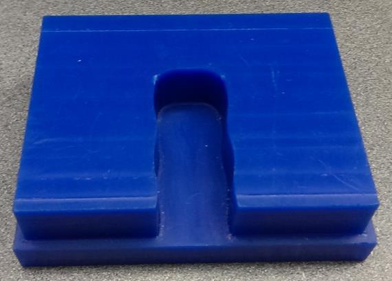
77 24b: Manufactured Tab 24c: Manufactured Slot 24d: Manufactured Hole Figure 24: Manufactured Parts with exaggerated Form Errors 66

78 The units in which the parts were created were mm. For the tab and slot (Figure 24b and 24c) the nominal width between the two planes was 20 units with a deviation of 1.0 mm on both sides of each plane. For pins and holes (Figure 24a and 24d), a nominal diameter of 30 units with a variation of 1.0 mm on the inside as well as towards the outside of the feature was incorporated. Table 6 shows the results for CMM testing and verification. Table 6: CMM Testing and Verification Results for a Plane, Circle and Cylinder Least Square Fits Results Least Square fit Ball dia Final value CMM Value % Error = Zone Plane Circle (dia) 0.02 Cylinder (dia) 0.41 The fifth column (in Table 6) is the fit values obtained from the CMM software. The values in column four are the values obtained from the least square algorithms after doing adjustments on the probe diameter. Column sixth shows the percentage errors between the results obtained from CMMs and the result obtained from doing least squares fit. We can note from Table 6 (column six) that the fit value obtained from the CMM and the one from the least square fit match very closely to each other. These results also lead to an assumption that CMM software computes the least square fits for doing feature fitting. 5.3 Comparative Studies with Manual Measurements In this mode of verification, manual measurements and verification are done by fitting a feature to the measured point cloud using proposed algorithms. Manufactured parts are measured manually using vernier caliper and screw gauge. Results obtained from manual measurements are compared in table 7 with the features fitted by the algorithm for verification. The same robotic arm CMM (Romer Series 3000i) was used for measuring points on the manufactured parts. The 67

79 points were measured in a way so that they spanned the measured surface. The parts used for measuring the point cloud were manufactured with built-in exaggerated form errors. Parts were created for a tab, slot, pin and hole (Figure 24). The units in which measurements were done is inches. Table 7a shows the results for manual measurements along with the CMM measurements and obtained values from algorithms. Table 7b shows how results of least square zones vary from the actual desired zone Table 7a: Manual Measurements and Verification Results Unconstrained One Sided and Minimum Zone Fits Minimum Zone CMM value Manual Measurement Algorithm Val Ball Diameter Final Val Min Zone Plane External Min Zone Plane Internal Min Zone Circle (from cad model) Min Zone Cylinder One Sided - Distance from datum (value in inches) CMM Manual Ball value Measurement Algorithm Val Diameter Final Val One sided Plane Min. Circumscribed circle (dia) (dia) 1.45(dia) (dia) Max. Inscribed circle (dia) (dia) (dia) (dia) Min. Circumscribed cyl. (dia) (dia) (dia) (dia) Max. Inscribed cyl (dia) (dia) (dia) (dia) 68

80 Table 7b: Percentage Error of Least Squares Zones to Desired Zones Unconstrained Minimum Zone Fits Least Squares Fit Manual Measurement Algorithm Val Ball Diameter Final Val % Error Min Zone Plane External Min Zone Plane Internal Min Zone Circle Min Zone Cylinder (from cad model) Column two of table 7 shows the value obtained by doing the fits using CMM software. Column three shows the values obtained by doing manual measurements of the manufactured test parts. Columns four and five show the values obtained by running the CMM point cloud through algorithms and adjustment for the measuring probe diameter. Final results of the algorithms with measuring probe diameter adjustments are summarized in sixth column (algorithm value + probe ball diameter adjustment). By comparing columns two, three and six, we can derive a conclusion that manual measurements are closer to algorithm measurements. It could be also deduced by comparing tables 6 & 7 that CMM measurements results are closer to those obtained by least squares fit. Hence, we can arrive at a conclusion that the CMM s are using least square fits. Looking at table 7b we can conclude that the zones obtained by least square fits differ from that obtained by an actual zone fit. 5.4 Application of Feature Fitting in GD&T Verification of different tolerance classes and simulation of datums require analyzing the same point cloud in different ways. Since, in a real part both datums and tolerance features lie on the same part, the measured point cloud can verify more than one tolerance classes. The following case studies demonstrate the usage of different feature fitting algorithms in evaluation 69

81 of machining variations to design tolerances. Two different cases are presented here to evaluate size, form and orientation tolerances by analyzing the same data sets in different ways Feature Fitting for Planar Features Two sets of point clouds were measured on the planar features of the manufactured part (cube) as shown in Figure 25. One set was measured on the Datum [A], and the other on the plane on the right hand side (controlled feature). Points are measured by a CMM on both the controlled and the controlling plane. Figure 25: Planar Features on a Part For orientation error (parallelism tolerance) verification in a planar feature (Figure 25), the planar feature should lie in a zone defined by two parallel planes such that the distance between the two planes is less than or equal to the tolerance specified by the designer. In order to verify this, a minimum zone fit for the planar feature, a one sided fit for the Datum feature are required. An unconstrained one sided plane fit is done on the point cloud that was measured on the controlling plane (datum) to establish the datum plane. An unconstrained minimum zone plane fit is done on the controlled plane. The distance between the planes of minimum zone fit is the estimation for the parallelism error. For verifying size tolerance, the part that is shown in 70

82 Figure 25 is considered as a Tab feature. A minimum zone unconstrained plane fit is done on this feature by combining both data sets. The distance between the planes of this zone can be compared to the original size tolerance, and an estimation of error can be obtained. For evaluation of the form tolerance, a minimum zone unconstrained plane fit is done on the point cloud for the datum. The distance between those planes will give the form error Feature Fitting for Cylindrical Feature A CMM measures a point cloud on both datum (controlling feature plane A) and the controlled feature (cylinder) as shown in Figure 26. Figure 26. Cylindrical Feature on a Part An unconstrained one sided plane is fitted for the datum if it is a planar feature. If the datum is an external cylindrical feature, a minimum circumscribed cylinder fit is used; otherwise (for the internal feature) a maximum inscribed cylinder is fitted. Next, an unconstrained one sided cylinder fit is done on the point cloud of the controlled feature depending upon whether it is an internal or external feature. Two points are measured along the axis of the fitted cylinder for the controlled feature such that the points lie on the extreme ends of the fitted feature. These points are then projected onto a plane perpendicular to the fitted datum feature. The distance between 71

83 the projections of these points in the projected plane gives the parallelism error. Size tolerance verification can be done by doing a one sided cylinder fit for the controlled feature. A maximum inscribed cylinder fit is done if the feature is an internal feature (e.g. a hole), or a minimum circumscribed cylinder fit is done if it is an external feature (e.g. a pin). The size of a one sided cylinder fit is used to verify the size tolerance. To verify a form tolerance, a minimum zone cylinder fit is done for the controlled feature. The radial distance between the two concentric cylindrical features gives the form error of the cylindrical feature. A detailed description of how different feature fitting algorithms should be utilized for verifying different types of tolerances and establishing datums can be found in V. Prabath work [28] 72

84 CHAPTER 6 CONCLUSION, LIMITATIONS/ASSUMPTIONS & FUTURE WORK 6.1 Conclusion A library of a comprehensive set of working feature fitting algorithms (Table 2) was created. Implementation of the algorithms was done in a software which complies with the standard [3]. The choice of algorithms was based on a few parameters such as accuracy, complexity of algorithm, and execution runtime of an algorithm. More weigh was given to accuracy and complexity parameters. All the unconstrained, constrained and least square feature-fitting algorithms were implemented and tested. The algorithms were implemented through a concept of object oriented programming so that if a better implementation of a certain feature fitting needs to replace the older one, it can be done without affecting the rest of the code modules. Testing of each algorithm type has revealed that a large number of data points affects the time of execution of algorithms. The computation time increases with an increase in the number of measured points, but not drastically for most of the cases. However, special cases like equally spaced points or algorithms like min circumscribed circle time increase with very large number of points. All of the algorithms employed for implementing different feature-fitting classes can be broadly divided into three stages: organization of data for initialization of the algorithm, running the algorithm in iterations, and finally comparing different solutions (from different iterations) to obtain the best one. This research work has made the following contribution A library of feature algorithms was developed A lot of research work was done by different researchers on different types of features fits. Some of the feature fit types had multiple existing algorithms proposed different researchers. All those algorithms were studied and compared. The algorithms which best 73

85 suited our criteria (accuracy, efficiency, robustness) were selected. All such existing algorithms for different types of fits were filtered and collected at one place for anyone to use and implement. Developed new feature fitting algorithms and modified existing ones Some of the feature fit types (like constrained fits) lacked existing efficient and robust existing algorithms. New algorithms were created for the fit types which lacked existing algorithms. In addition to lack of existing algorithms, some algorithms were either failing for special cases or were not efficient enough. These existing algorithms were modified accordingly to make them more robust and efficient. Table 8 shows which algorithms existed, which were modified and which were created new Implemented a software for feature fitting algorithm in form of a function library Software of these algorithms was made in form of a library. The library was made in form of function API s so that anyone can easily integrate these function calls into their own software. Functions were developed in an object oriented style independent manner. This was done so that the library could be expanded or a function could be modified without affecting other function implementations. Analyzed and tested CMM software Several test parts with exaggerated form errors were manufactured. These parts were measured using CMMs. The point cloud was analyzed using CMM software as well as using the algorithms developed and manual measurements. The results obtained were compared and deductions about CMM software were made. After comparing the results it was observed that results obtained from a CMM matched closely with those obtained from least square fits. Thus, it can be assumed that the CMMs are using least square fits. Table 8: Work Done on Each Algorithm Algorithm Type Reference Work Done 74

86 Least Square Line Fit Least Square Circle Fit Least Square Plane Fit 75 Label 1A 2A 3A Existing Modified to generate initial guess Existing Modified to generate initial guess Existing Modified to generate initial guess Least Square Cylinder Fit 4A Existing Unconstrained One Sided Line Fit 1B Created New Unconstrained Circumscribed Circle Fit 2B - 1 Unconstrained Inscribed Circle Fit 2B - 2 Adaptation of an existing algorithm Adaptation of an existing algorithm Unconstrained One Sided Plane Fit 3B Created New Unconstrained Circumscribed Cylinder Fit 4B - 1 Unconstrained Inscribed Cylinder Fit 4B - 2 Existing Modified to get a good start point Existing Modified to get a good start point Unconstrained Minimum Zone Line Fit 1C Created New Unconstrained Minimum Zone Circle Fit Unconstrained Minimum Zone External Plane Fit Unconstrained Minimum Zone Internal Plane Fit Unconstrained Minimum Zone Cylinder Fit 2C 3C - 1 3C - 2 4C Adaptation of an existing algorithm Existing Modified to give better results Created New Existing Modified to get a good start point Constrained One Sided Line Fit 1D Created New Constrained Circumscribed Circle Fit 2D - 1 Created New Constrained Inscribed Circle Fit 2D - 2 Created New Constrained One Sided Plane Fit 3D Created New Constrained Circumscribed Cylinder Fit 4D - 1 Created New Constrained Inscribed Cylinder Fit 4D - 2 Created New Constrained Minimum Zone Line Fit 1E Created New Constrained Minimum Zone Circle Fit 2E Created New

87 Unconstrained Minimum Zone External Plane Fit Unconstrained Minimum Zone Internal Plane Fit 3E - 1 3E - 2 Created New Created New Unconstrained Minimum Zone Cylinder Fit 4E Created New It is observed that the uniformity of sampling scheme would also affect the results of least squares fit algorithms. A non-uniform scheme will shift the fitted least square feature towards a denser zone of the measured point cloud. This will change the orientation as well as location of the fitted feature. Figure 11 shows the case of rotating a non-uniform data set. When a feature (circle) was fitted to these rotated data sets it was observed all of the fitted circles vary in their position. In case of unconstrained and constrained one sided and minimum zone fit, the effect of outliers is minimized by taking the direction of fitting into consideration. 6.2 Limitations/Assumptions The algorithms developed during this research have certain limitations associated with them. These limitations originate from certain assumptions that were made regarding the sampling scheme and type of data that goes into these algorithms. An assumption that is common to all the algorithms proposed in this research is that measured points should span the surface of the feature. Moreover, the time taken by algorithms goes up with the number of measured points as well as the type of fit to be done. A constrained circle fit will take less time than a unconstrained circle fit for same number of measured points. The Unconstrained cylinder fit takes more time than the unconstrained plane fit for a given number of measured points because the number of parameters to locate a cylinder is greater than the number required for a plane. Following are the assumptions/limitations made during the development of this library. 76

88 Least Square Fits Least square fits are done using the NPL [9] approach. Since, least squares fits work by minimizing the sum of squares of distance to the initial feature, data sets with a high number of outlier points affect the solutions of the least square fits. For doing a least square cylinder fit, it was assumed that the initial estimates of cylinder parameters (points on the axis, radius and direction vector of axis) would be provided (from cad model). This brings a limitation that if the initial estimates are too far off from the required fitted feature, it will affect the results given by the least square fit. Unconstrained One Sided Fits One sided line and circle fits work with 2D points cloud only whereas, one sided plane and cylinder fit works with 3D point cloud. It was assumed that for doing one sided line and plane fits an initial estimate of direction vector from which the fitting is done would be provided along with the point cloud. It was also assumed that initial estimate for cylinder parameters (points on the axis, radius and direction vector of axis) would be provided (from cad model). Since, these initial estimates initialize the algorithms their values affect the results of the fit type. The closer these estimates are to the fit type the faster and more accurately the algorithms work. Unconstrained Minimum Zone Fits Zone line and circle fits work for 2D points only and zone plane and cylinder fits work for 3D points only. External and internal zone plane fits requires three measured points for establishment of an initial reference plane. Since, the zone plane fit is done with reference to this plane, the results of the zone plane fit are limited by the orientation of the initial reference plane. Zone cylinder fit also needs the estimate of initial cylinder parameters and the results of the cylinder fit are affected by the initial estimates. In 77

89 addition to these limitations, all zone fits must have the minimum number of required points on the feature forming the zone as dictated by their geometric entities. Constrained One Sided Fits Constrained one-sided fits require the direction vector of the constraining feature for doing the fit. If the direction vector of the constraining feature is not well defined or is just an approximation it will affect the results of the constrained fits. This effect of direction will vary as how bad the approximation is. A very bad approximation can alter the results by substantial amount. Constrained one-sided fits were limited for doing fits with respect to parallel and perpendicular features only. It was assumed that for doing a constrained one-sided line and plane fit, the direction vector of the constraining feature along with the estimate of initial direction of fitting would be provided. Constrained Minimum Zone Fits Constrained minimum zone fits results are also affected by accuracy and definition of the constraining features. Constrained minimum zone fits for a line and a circle works for 2D point s only, and constrained minimum zone fit for a plane and a cylinder works with 3D point s only. Apart from limitations, the execution time of algorithms is also important in evaluating their effectiveness. It was observed that the time required for algorithms to execute depends upon: The number of parameters associated with the feature/ type of feature to be fitted. The number of points measured (point cloud). What type of fit it is (constrained, unconstrained or least squares). Table 9 summarizes the time that different algorithms took for a set of 100 measured points. These times are not CPU times but approximate times observed during the execution of 78

90 algorithms. Table 10 shows the complexity associated with each algorithm type. The complexity is calculated in big O terms. Table 9: Algorithm Execution Times for 100 Measured Points Fit Type Least Squares Algorithm and their Reference Numbers Time Taken to Execute (in seconds) 1A: line 2 approx. 2A: circle 2 approx. 3A: plane 3 approx. 4A: cylinder 3 approx. 1B: line 3 approx. Unconstrained One Sided Fits 2B-1: circumscribed circle 3 approx. 2B-2: inscribed circle 3B: plane 4 approx. 4B-1: circumscribed cylinder 4 approx. 4B-2: inscribed cylinder 1C: line zone 3.5 approx. Unconstrained Minimum Zone Fits 2C: annular zone 3.5 approx. 3C-1 external plane zone 4.2 approx. 3C-2 internal plane zone 4C: cylinder zone 4.2 approx. 1D: line 2 approx. Constrained One Sided Fits Constrained Minimum Zone 2D-1: circumscribed circle 2D-2: inscribed circle 2 approx. 3D: plane 2.5 approx. 4D-1: circumscribed cylinder 3 approx. 4D-2: inscribed cylinder 1E: line zone 2 approx. 79

91 Fits 2E: annular zone 2 approx. 3E-1 external plane zone 3 approx. 3E-2 internal plane zone 4E: cylinder zone 3 approx. Table 10: Complexity Associated with Each Algorithm Algorithm Type Reference Label Complexity Least Square Line Fit 1A O(n^2) Least Square Circle Fit 2A O(n^2) Least Square Plane Fit 3A O(n^2) Least Square Cylinder Fit 4A O(n^2) Unconstrained One Sided Line Fit 1B O(n) Unconstrained Circumscribed Circle Fit 2B - 1 O(n^2) Unconstrained Inscribed Circle Fit 2B - 2 O(n^2) Unconstrained One Sided Plane Fit 3B O(n^2) Unconstrained Circumscribed Cylinder Fit 4B - 1 O(n^2) Unconstrained Inscribed Cylinder Fit 4B - 2 O(n^2) Unconstrained Minimum Zone Line Fit 1C O(n^2) Unconstrained Minimum Zone Circle Fit 2C O(n^2) Unconstrained Minimum Zone External Plane Fit 3C - 1 O(n^2) Unconstrained Minimum Zone Internal Plane Fit 3C - 2 O(n^2) Unconstrained Minimum Zone Cylinder Fit 4C O(n^2) Constrained One Sided Line Fit 1D O(n) 80

92 Constrained Circumscribed Circle Fit 2D - 1 O(n) Constrained Inscribed Circle Fit 2D - 2 O(n) Constrained One Sided Plane Fit 3D O(n^2) Constrained Circumscribed Cylinder Fit 4D - 1 O(n^2) Constrained Inscribed Cylinder Fit 4D - 2 O(n^2) Constrained Minimum Zone Line Fit 1E O(n) Constrained Minimum Zone Circle Fit 2E O(n) Unconstrained Minimum Zone External Plane Fit 3E - 1 O(n) Unconstrained Minimum Zone Internal Plane Fit 3E - 2 O(n) Unconstrained Minimum Zone Cylinder Fit 4E O(n^2) 6.3 Future Work Future work involves further testing of the proposed algorithms with a variety of test cases and modifications of algorithms if necessary. Also, the feature library needs to be further expanded to accommodate more feature types (spheres, cones etc.). If a better, algorithm or method is found to do a certain type of fit, then the existing ones need to be replaced with a new tested ones. Tolerance classes like profile and run out tolerances are right now not supported by the library. Development and implementation of these algorithm classes will also be one the tasks for future. Another important aspect of the library is the usage of the library. Once the various feature fits are available, they need to be used in a certain order or combination in order to correctly verify the tolerance classes and datum simulation. The next task would be to interpret the standard [3] and using this library to make recommendations. These recommendations should specify the 81

93 correct combination or sequence of these feature-fitting functions for verification of different tolerance classes and datum simulation. 82

94 REFERENCES [1] GIDEP 1988 GIDEP Alert X1-A-88-02, Welber R, CMM Form Tolerance Algorithm Testing, GIDEP DOD, Washington D.C. [2] [3] ASME Y14.5, 1994, Dimensioning and Tolerancing, The American Society of Mechanical Engineers, New York. [4] [5] hina-3d-coordinate-measurement-machine-leader-cmm-.html [6] Bosch John A., 1995, Coordinate Measuring Machine and Systems, Marcel Dekker, Inc, ISBN , Volume 42, xi, 444 [7] Hocken, Robert J and Pereira, Paulo H, Coordinate measuring machines and systems, 2012, 2nd ed., Manufacturing engineering and materials processing, ISBN , Volume 76 [8] Zhengshu Shen, Jami J. Shah, Joseph K. Davidson, Analysis Neutral Data Structure for GD&T, J Intell Manuf (2008) 19: [9] Alistair B Forbes, 1991 (Revised Edition), Least Squares Best Fit Geometric Elements, NPL Report DITC 140/89. [10] Craig M. Shakarji, 1998, Least Squares Fitting Algorithms of the NIST Algorithm Testing System, Journal of research of the National Institute of Standards and Technology, 103(6). [11] Carr K, Ferreira P, 1995, Verification of form tolerances, part II: cylindricity and straightness of a median line. Precision Engineering, 17(2), pp [12] Hsinyi Lai, Wenyuh Jywe, Cha OKuang Chen, et al., 2000, Precision modeling of form errors for cylindricity evaluation using genetic algorithms. Precision Engineering, 24, pp [13] Q. Zhang, K.C. Fan, Z. Li, 1999, Evaluation method for spatial straightness errors based on minimum zone condition. Precision Engineering, 23, pp [14] N. Venkaiah, M.S. Shunmugam, 2007, Evalaution of form data using computational geometric techniques-part II: Cylindricity error. International Journal of Machine Tools & Manufacture, 47, pp [15] S. Hossein Cheraghi, Guohua Jiang, Jamalsheikh Ahmad, 2003, Evaluating the geometric characteristics of cylindrical features. Precision Engineering, 27, pp

95 [16] Craig M. Shakarji, 2004, Reference Algorithm for Chebyshev and One-Sided Data Fitting for Coordinate Meteorology. CIRP Annals Manufacturing Technology, 53(1), pp [17] Dawit H. Endrias, His-Yung Feng, Ji Ma, Lihui Wang, M. Abu Taher, 2012, A combinatorial optimization approach for evaluating minimum-zone spatial straightness errors. Measurement, 45, pp [18] Li Xiuming, Shi Zhaoyao, 2008, Application of convex hull in the assessment of roundness error. International Journal of Machine Tools & Manufacture, 48, pp [19] Moon-Kyu Lee, 2009, An enhanced convex-hull edge method for flatness tolerance evaluation. Computer-Aided Design, 41, pp [20] Lei Xianqing, Song Hongwei, Xue Yujun, Li Jishun, Zhou Jia, Duan Mingde, 2011, Method for cylindricity evaluation error evalaution using Geometry Optimization Searching Algorithm, Measurement, 44, pp [21] GE Q, Chen B, Smith P, Menq C. H, Tolerance Specification and Comparative Analysis for Computer-Integrated Dimensional Inspection, International Journal of Production Research, ISSN , 09/1992, Volume 30, Issue 9, pp [22] Bhat Vinod, De Meter, Edward C, An Analysis of the Effect of Datum-Establishment Methods on the Geometric Errors of Machined Features, International Journal of Machine Tools and Manufacture, ISSN , 2000, Volume 40, Issue 13, pp [23] N. Venkaiah, M.S. Shunmugam, 2007, Evalaution of form data using computational geometric techniques-part I: Circularity error. International Journal of Machine Tools & Manufacture, 47, pp [24] Gyula Hermann, Robust Convex Hull-based Algoritm for Straightness and Flatness Determination in Coordinate Measuring, Acta Polytechnica Hungarica, ISSN , 12/2007, Volume 4, Issue 4, pp [25] W.H. Press, S.A. Teukolsky, W.T. Vetterling, B.P. Flannery, "Numerical Recipes in C", Cambridge Univ. Press. [26] Thomas H. Cormen, Charles E. Leiserson, Ronald L. Rivest, Clifford Stein, 2001, Introduction to Algorithms (2nd ed.), MIT Press and McGraw-Hill, pp [27] K. L. Clarkson, K. Mehlhorn, and R. Seidel. Four results on randomized incremental constructions. Comput. Geom. Theory Appl., 3(4): , [28] Vemullapali Parbath, Jami Shah, J.K. Davidson, 2013, Reconciling the Differences Between Tolerance Specification and Measurement Methods. Proceedings of the ASME 2013 International Manufacturing Science and Engineering Conference, MSEC [29] G.T. Anthony, B.P. Butler, M.G. Cox, A.B. Forbes, S.A. Hannabay, P.M. Harris, 1993, Chebyshev Refernce Software for the Evaluation of Coordinate Measuring Machine Data, Commission of the European Communities, EUR EN 84

96 [30] Shakarji C.M, Srinivasan, V, 2012, Fitting Weighted Total Least-Squares Planes and Parallel Planes to Support Tolerancing Standards. Proceedings of the ASME 2012 International Design Engineering Technical Conferences & Computers and Information in Engineering Conference, Chicago, August [31] Vijay Srinivasan, Craig M. Shakarji, Edward P. Morse, 2012, On the Enduring Appeal of Least-Squares Fitting in Computational Coordinate Metrology. J. Comput. Inf. Sci. Eng, Volume 12, Issue 1,

97 APPENDIX A: FUNCTIONS DEFINITIONS OF THE LIBRARY 86

98 Least Square Line Fit: Function Call: line fit has two functions calls one for 2D and one for 3D. The Functions calls are listed below: // Least Square line 2D fitting bool LeasSquareLine2D(const matrix<t>& A, matrix<t>& B); //least square line in 3D fitting bool LeasSquareLine3D(const matrix<t>& A, matrix<t>& B); Input: The Input to the line fit function is a matrix (A) which contains 2D or 3D coordinates of the measured points (Figure 27). Output: Output to the line fit function is a matrix (B). First line of B contains the contain coordinates of a point on line and second line contains component of the direction vector of the fitted line. Least Square Plane Fit: Function Call: The Functions calls for the plane fit (in 3D) is listed below // Least Square Plane fitting bool LeasSquarePlane(const matrix<t>& A, matrix<t>& B); Input: The Input to the plane fit function is a matrix (A) which contains 3D coordinates of the measured points (Figure 27). Output: Output to the plane fit function is a matrix (B). First line of B contains the contain coordinates of a point on plane and second line contains component of the direction vector of normal to the fitted plane. 87

99 Least Square Circle Fit: Function Call: Circle fit has two functions calls one for 2D and one for 3D. The Functions calls are listed below: //Least Square Circle 2D Fitting bool LeasSquareCircle2D (const matrix<t>& A, matrix<t>& B, double& C); //Least Square Circle 3D fitting bool LeasSquareCircle3D (const matrix<t>& A, matrix<t>& B, double& C); Input: The Input to the circle fit function is a matrix (A) which contains 2D or 3D coordinates of the measured points (Figure 27). Output: Output to the circle fit function is a matrix (B) and parameter C. First line of B contains the contain coordinates of the center of the fitted circle in case of 2D. In case of 3D circle fit, first line of matrix B contains center of the fitted circle. Second line contains components of the vector, normal to the plane of the fitted circle. Parameter C contains the radius of the fitted circle. Least Square Cylinder Fit: Function Call: The Functions calls for the cylinder fit (in 3D) is listed below //Least Square Cylinder fitting bool LeasSquareCylinder (const matrix<t>& A, matrix<t>& D, double& C, matrix<t>& B, double& R); Input: The Input to the cylinder fit function are matrices A & D and parameter C. Matrix D contains 3D coordinates of the measured points. Matrix A contains an initial estimate of a point on the axis of cylinder in the first line. Second line of matrix A contains an initial estimate of direction vector of the axis of cylinder. Parameter C contains an initial estimate of the radius of the fitted cylinder (Figure 28). Output: Output to the cylinder fit function is a matrix (B) and parameter R. First line of B contains the contain coordinates of a point on the axis of the fitted cylinder. Second line 88

100 contains component of the direction vector of the axis of the fitted cylinder. Parameter R contains the radius of the fitted cylinder. Figure 27 a: Input File for 2D Points Figure 27 b: Input File for 3D Points Figure 27: Input File for Line, Plane and Circle Fit Figure 28: Input File for Cylinder Fit Unconstrained One Sided Line Fit: Function Call: line fit his done in 2D. The Functions calls are listed below: 89

101 // One sided line 2D fitting bool Line_Fit_2D(const matrix<t>& A, matrix<t>& B, matrix<t>& D); Input: The Input to the line fit function is a matrix (A) which contains 2D coordinates of the measured points and a matrix (D), which contains the direction from which the fitting should be done (Figure 29). Output: Output to the line fit function is a matrix (B). First line of B contains the contain coordinates of a one point on line. Second line contains the coordinates of the second point on the fitted line. Figure 29: Input File for One Sided Line Fit Unconstrained One Sided Plane Fit: Function Call: The Functions calls for the plane fit (in 3D) is listed below //One sided plane fit bool Plane_Fit_3D(const matrix<t>& A, matrix<t>& B, matrix<t>& D, std::vector<double>& direc_vec); Input: The Input to the plane fit function is a matrix (A) which contains 3D coordinates of the measured points and a matrix (D), which contains the direction from which the plane fit should be done (Figure 30). 90

102 Output: Output to the plane fit function is a matrix (B) and a vector (direc_vec). First, Second and Third line of B contains the coordinates of points forming the fitted plane. direc_vec contains the vector components of the normal to the fitted plane. Figure 30: Input File for One Sided Plane Fit Unconstrained One Sided Circle Fit: Function Call: Circle fit has two functions calls one for minimum circumscribed and one for maximum inscribed circle fit. The Functions calls are listed below: //Minimum circumscribed circle bool Min_Circum_Fit_2D(const matrix<t>& A, matrix<t>& B); //Maximum Inscribed circle bool Max_Ins_Fit_2D(const matrix<t>& A, matrix<t>& B); Input: The Input to the circle fit function is a matrix (A) which contains 2D coordinates of the measured points (Figure 27 a). Output: Output to the circle fit function is a matrix (B). First line of B contains the contain coordinates of the center of the fitted circle in case of 2D. Second line of the B contains the radius of the fitted circle. Unconstrained One Sided Cylinder Fit: 91

103 Function Call: The Functions calls for the cylinder fit (in 3D) are given below. Cylinder fit also has two variations, maximum inscribed cylinder and minimum circumscribed cylinder. //Minimum circumscribed cylinder bool Min_Cyl_Fit_3D(const matrix<t>& A, const matrix<t>& D, matrix<t>& B); //Maximum Incribed cylinder bool Max_Cyl_Fit_3D(const matrix<t>& A, const matrix<t>& D, matrix<t>& B); Input: The Input to the cylinder fit function is matrices A & D. Matrix A contains 3D coordinates of the measured points. Matrix D contains an initial estimate of a point on the axis of cylinder in the first line. Second line of matrix A contains an initial estimate of direction vector of the axis of cylinder. Third line of matrix D contains an initial estimate of the radius of the fitted cylinder (Figure 28). Output: Output to the cylinder fit function is a matrix (B). First line of B contains the contain coordinates of a point on the axis of the fitted cylinder. Second line contains component of the direction vector of the axis of the fitted cylinder. Third line contains the radius of the fitted cylinder. Unconstrained Minimum Zone Line Fit: Function Call: line fit his done in 2D. The Functions calls are listed below: // Least Square line 2D fitting bool Min_Zone_Line_Fit_2D(const matrix<t>& A, matrix<t>& B, double& Distance); Input: The Input to the line fit function is a matrix (A) which contains 2D coordinates of the measured points (Figure 27 a). Output: Output to the line fit function is a matrix (B) and parameter Distance. First and Second line of B contains the contain coordinates of points forming one side of the fit. Third line 92

104 contains the coordinates of the point forming other side of the fit. Parameter Distance contains distance of the zone fit. Unconstrained Minimum Zone Plane Fit: Function Call: The Functions calls for the plane fit (in 3D) are outlined below. Plane fit has two variations i.e. External zone plane fit and internal zone plane fit. double& double& //for doing external fit bool Min_Zone_Plane_Fit_3D_Ex(const matrix<t>& A, matrix<t>& B, Distance, std::vector<double>& direc_vec); //for doing internal fit bool Min_Zone_Plane_Fit_3D_In(const matrix<t>& A, matrix<t>& B, Distance, std::vector<double>& direc_vec); Input: The Input to the plane fit function is a matrix (A) which contains (in 3D) coordinates of the measured points. For the external plane fit, first line contains the number of points for initial estimate of least square fits as well as the count of number of measured points (Figure 31 b). For an internal plane fit, first line contains the count for number of points for initial estimate of least square fit. It also contains the count for points measured on right hand side and left hand side points (Figure 31 a). Output: Output to the plane fit function is a matrix (B), a vector (direc_vec) and a parameter Distance. First, Second and Third line of B contains the coordinates of points forming one side of fitted zone plane. Fourth line of the B contains coordinates of a point forming other side of the fitted zone. direc_vec contains the vector components of the normal to the fitted plane. Distance contains the distance of the fitted zone 93

105 Figure 31 a: Input File for Internal Plane Figure 31 b: Input File for External Plane Figure 31: Input File for Unconstrained Minimum Zone Plane Fit Unconstrained Minimum Zone Circle Fit: Function Call: Circle fit is done in 2D. The Functions call for the circle is given below: // Minimum Zone Circle 2D fitting bool Min_Zone_Circle_Fit_2D(const matrix<t>& A, matrix<t>& B); Input: The Input to the circle fit function is a matrix (A) which contains 2D coordinates of the measured points (Figure 27 a). Output: Output to the circle fit function is a matrix (B). First line of B contains the contain coordinates of the center of the fitted circle in case of 2D. Second line of the B contains the minimum and maximum radius of the fitted zone circle. Unconstrained Minimum Zone Cylinder Fit: Function Call: The Functions call for the cylinder fit (in 3D) are given below. //Minimum Zone Cylindern 3D fitting bool Min_Zone_Cyl_Fit_3D(const matrix<t>& A, const matrix<t>& D, matrix<t>& B); Input: The Input to the cylinder fit function is matrices A & D. Matrix A contains 3D coordinates of the measured points. Matrix D contains an initial estimate of a point on the axis of 94

106 cylinder in the first line. Second line of matrix A contains an initial estimate of direction vector of the axis of cylinder. Third line of matrix D contains an initial estimate of the radius of the fitted cylinder (Figure 28). Output: Output to the cylinder fit function is a matrix (B). First line of B contains the contain coordinates of a point on the axis of the fitted cylinder. Second line contains component of the direction vector of the axis of the fitted cylinder. Third line contains the minimum and maximum radius of the fitted cylinder. Constrained One Sided Line Fit: Function Call: line fit his done in 2D. Constrained line fit has two variations, one with respect to a parallel line and other with respect to a perpendicular line. The Functions calls are listed below: //parallel to al line bool Cons_Line_Fit_2D_parl(const matrix<t>& A, matrix<t>& B, matrix<t>& D); //perpendicular to a line bool Cons_Line_Fit_2D_pd(const matrix<t>& A, matrix<t>& B, matrix<t>& D); Input: The Input to the line fit function are matrices A & D. Matrix A contains 2D coordinates of the measured points. Matrix D contains the direction from which the fitting should be done and the equation of the constraining line (Figure 32). Output: Output to the line fit function is a matrix (B). First line of B contains the contain coordinates of a one point on line. Second line contains the coordinates of the second point on the fitted line. 95

107 Figure 32: Input File for Constrained One Sided Line Fit Constrained One Sided Plane Fit: Function Call: The Functions calls for the plane fit (in 3D) are listed below. Plane fits are done with respect to a constraining parallel plane. //One sided plane fit bool Cons_Plane_Fit_3D(const matrix<t>& A, matrix<t>& B, matrix<t>& D); Input: The Input to the plane fit function is a matrix A and D. A contains 3D coordinates of the measured points. First line of D contains the direction from which the plane fit should be done. Second line of D contains the equation of the constraining plane (Figure 33). Output: Output to the plane fit function is a matrix (B). First line of B contains the vector components of the normal to the fitted plane. Second line of B contains the coordinates of point forming the fitted plane. 96

108 Figure 33: Input File Format for Constrained One Sided Plane Fit Constrained One Sided Circle Fit: Function Call: Circle fit has two functions calls one for minimum circumscribed and one for maximum inscribed circle fit. Circle fit is done with respect to its true position (center) being constrained. The Functions calls are listed below: //Constrained Minimum circumscribed circle bool Cons_Min_Circum_Fit_2D(const matrix<t>& A, matrix<t>& B, matrix<t>& D); //Constrained Maximum Inscribed circle bool Cons_Max_Ins_Fit_2D(const matrix<t>& A, matrix<t>& B, matrix<t>& D); Input: The Input to the circle fit function is matrices A & D. A contain 2D coordinates of the measured points. D contains estimates of the true position (center) of the fitted circle (Figure 34). Output: Output to the circle fit function is a matrix (B), which gives the radius of the fitted circle. 97

109 Figure 34: Input File Format for Constrained Circle Fit Constrained One Sided Cylinder Fit: Function Call: Cylinder fit also has two variations, maximum inscribed cylinder and minimum circumscribed cylinder. Cylinder fit can be done with respect to constraining parallel line or normal to a constraining plane. The Functions calls for the cylinder fit (in 3D) are given below. //Constrained Minimum circumscribed cylinder - parallel to a linb bool Cons_Min_Cyl_Fit_3D_Parl(const matrix<t>& A, const matrix<t>& D, matrix<t>& B); //Constrained Maximum Incribed cylinder - parallel to a line bool Cons_Max_Cyl_Fit_3D_Parl(const matrix<t>& A, const matrix<t>& D, matrix<t>& B); Input: The Input to the cylinder fit function is matrices A & D. Matrix A contains 3D coordinates of the measured points. Matrix D contains the direction vector of the constraining line (in 3D) or normal vector to the constraining plane (Figure 35). Output: Output to the cylinder fit function is a matrix (B). First line of B contains the contain coordinates of a point on the axis of the fitted cylinder. Second line contains radius of the fitted cylinder. Direction vector of the axis of the fitted cylinder comes from the constraining direction vector. 98

110 Figure 35: Input File Format for Constrained Cylinder Fit Constrained Minimum Zone Line Fit: Function Call: line fit his done in 2D. Constrained line fit has two variations, with respect to constraining parallel line and with respect to a constraining perpendicular line. The Functions calls are listed below: // Constrained Min Zone line fitting for a given parallel line bool Cons_Min_Zone_Line_Fit_2D_Parl(const matrix<t>& A, matrix<t>& B, matrix<t>& C, double& Distance); // Constrained Min Zone line fitting for a given perpendicular line bool Cons_Min_Zone_Line_Fit_2D_Perpnd(const matrix<t>& A, matrix<t>& B, matrix<t>& C, double& Distance); Input: The Input to the line fit function is matrices A & C. Matrix A contains 2D coordinates of the measured points. Matrix C contains the equation of the constraining line (Figure 36). Output: Output to the line fit function is a matrix (B) and parameter Distance. First line of B contains the contain coordinates of points forming one side of the fit parallel/perpendicular to constraining line. Second line contains the coordinates of the point forming other side of the fit. Parameter Distance contains distance of the zone fit. 99

111 Figure 36: Input File Format for Constrained Minimum Zone Line Fit Constrained Minimum Zone Plane Fit: Function Call: The Functions calls for the plane fit (in 3D) are outlined below. Plane fit has two variations i.e. External zone plane fit and internal zone plane fit. Plane Fit can also be done parallel or perpendicular with respect to a constraining plane. //Constrained Min Zone Plane fitting for a given parallel Plane bool Cons_Min_Zone_Plane_Fit_3D_Ex_Parl(const matrix<t>& A, matrix<t>& B, matrix<t>& C, double& Distance); //Constrained Min Zone Plane fitting for a given perpendicular Plane bool Cons_Min_Zone_Plane_Fit_3D_Ex_Perpend(const matrix<t>& A, matrix<t>& B, matrix<t>& C, double& Distance); //Constrained Min Zone Plane fitting for a given parallel Plane bool Cons_Min_Zone_Plane_Fit_3D_In_Parl(const matrix<t>& A, matrix<t>& B, matrix<t>& C, double& Distance); Input: The Input to the plane fit function is a matrix A & C. A contains (in 3D) coordinates of the measured points. C contains the equation of the constraining plane (Figure 37). Output: Output to the plane fit function is a matrix (B), and a parameter Distance. In case of parallel constraining plane, first line of B contains the coordinates of a point forming one side of fitted zone plane. Second line of the B contains coordinates of a point forming other side of the fitted zone. In case of perpendicular constraining plane, first and second line of B contains the coordinates of points forming one side of fitted zone 100

112 plane. Third line of the B contains coordinates of a point forming other side of the fitted zone. Distance contains the distance of the fitted zone Figure 37: Input File Format for Constrained Minimum Zone Plane Fit Constrained Minimum Zone Circle Fit: Function Call: Circle fit is done with respect to its true position (center) being constrained. The Functions calls are listed below: // Constained Minimum Zone Circle 2D fitting bool Cons_Min_Zone_Circle_Fit_2D(const matrix<t>& A, matrix<t>& B, matrix<t>& C); Input: The Input to the circle fit function is matrices A & C. A contain 2D coordinates of the measured points. C contains estimates of the true position (center) of the fitted circle (Figure 34). Output: Output to the circle fit function is a matrix (B), which gives the minimum and maximum radius of the fitted zone circle. Constrained Minimum Zone Cylinder Fit: Function Call: Cylinder fit can be done with respect to constraining parallel line or normal to a constraining plane. The Functions calls for the cylinder fit (in 3D) are given below. 101