X.-Z Liu et al. / Computers in Industry 58 (2007)

Transcription

1

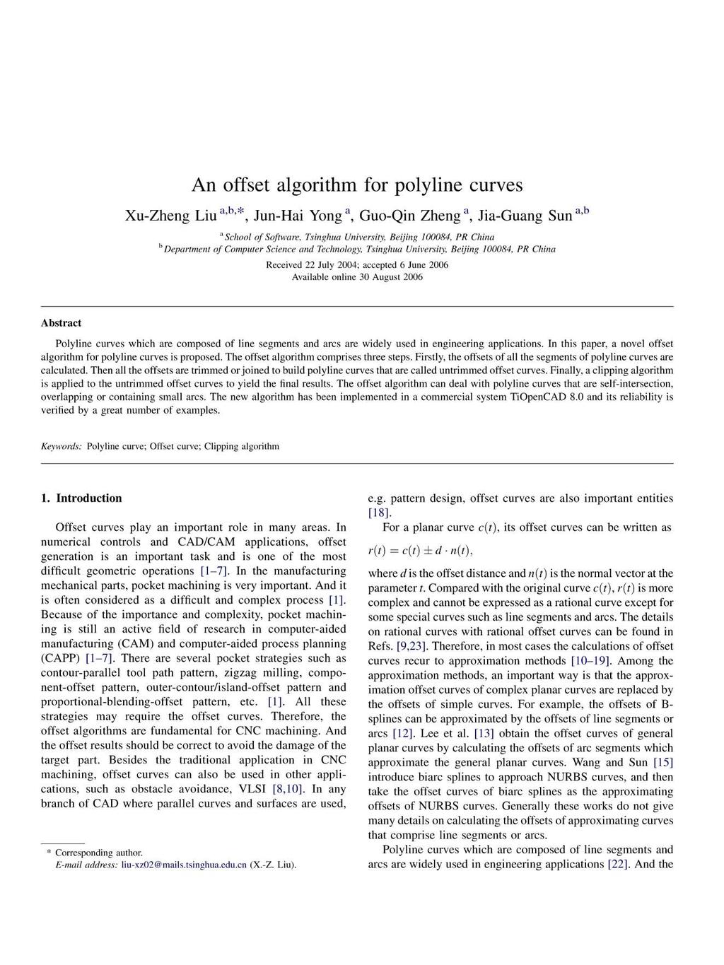
2 X.-Z Liu et al. / Computers in Industry 58 (2007) Fig. 1. The offset results from (a) AutoCAD2004, (b) AutoCAD2002, and (c) the algorithm in this paper. segments of a polyline curve may organize complicatedly. On the one hand, the two neighboring segments of a polyline curve are connected with only G 0 continuity. On the other hand, there may be self-intersection and overlapping among its segments. Although the offset curves of arcs and line segments are arcs and line segments, respectively, there still exist some problems to calculate the offsets of polyline curves. For instance, sometimes only parts of offset curves can be obtained or the offset curves may intersect with the original polyline curves. To address the problems clearly, we take Figs. 1 and 2 as examples. In these examples, the thick curves are original polyline curves and the thin curves are the offset curves on both sides of the original curves. In Fig. 1, the original curve is a closed polyline curve that contains two small arcs. As shown in Fig. 1(a), the commercial software AutoCAD 2004 produces two offset curves, and AutoCAD 2002 cannot produce any offset curves (Fig. 1(b)). In Fig. 2, the original polyline curve is more complex than that in Fig. 1, and it has many self-intersection points. The offset curves from AutoCAD 2004 have some obvious errors since they have intersection points with the original curve (Fig. 2(a)). And only parts of the offset curves can be obtained from AutoCAD 2002 (Fig. 2(b)). A probable reason for this phenomenon may come from the difficulty to deal with complex organization among the segments of a polyline curve. Therefore, a better offset algorithm for polyline curves is needed to solve the above problems. In CNC machining, many boundaries of the parts are polyline curves or approximated by polyline curves. For example, the internal boundary of the part illustrated in Fig. 3 is a polyline that is composed of three circular arc and five line segments. If the offsets of the boundary are obtained, the tool paths can be generated easily. And we will give two examples to generate tool paths in Section 6. Furthermore, the offset algorithm for polyline curves is not limited to the polyline curves themselves and it can also provide a blue print for the Fig. 2. The offset results from (a) AutoCAD2004, (b) AutoCAD2002, and (c) the algorithm in this paper. Fig. 3. The part to be machined. approximation offsets of other complex planar curves. Actually, the methods mentioned in Refs. [12,13] and [15] have adopted the strategy that the offsets of complex planar curves are replaced by the offsets of polyline curves. However, to our best knowledge, there are not many research works [20,21] aiming at the offset algorithm for polyline curves except for the commercial software AutoCAD. Choi and Park [20] give an algorithm for point-sequence curves (PS-curves) obtained by intersecting a sculptured surface with a plane. PScurves including only line segments can be regarded as polyline curves. Li and Ye [21] study the method on non-selfintersection polyline curves which do not involve curves that are self-intersection, overlapping or containing small arcs. In this paper, an offset algorithm for polyline curves is presented and its target is to obtain all the offset curves. And the offset algorithm can deal with polyline curves that are closed, self-intersection, overlapping or containing small arcs. For example, Figs. 1(c) and 2(c) illustrate the offset results from the algorithm proposed in this paper. These results are much better than those from AutoCAD. The main idea of this offset algorithm is described briefly as follows. Firstly, the offsets of all the segments of a polyline curve are calculated. Then the offsets are joined into a polyline curve that is called an untrimmed offset curve. The untrimmed offset curve includes all the offsets of the original curve. But it may contain many self-intersecting loops or intersect with the original curve. Finally, the offset results are obtained after the application of a clipping algorithm to the untrimmed offset curve. We also prove that the clipping algorithm does not cut out the untrimmed offset curve overmuch. Thus the offset algorithm is guaranteed theoretically to gain all the offset curves. The remaining part of the paper is organized as follows. Some basic definitions are given in Section 2. An algorithm to get an untrimmed offset curve is proposed in Section 3, where only the polyline curves that are open and not overlapping are considered. Section 4 presents a clipping algorithm for untrimmed offset curves and Section 5 discusses complex

3 242 X.-Z Liu et al. / Computers in Industry 58 (2007) polyline curves that are closed, overlapping or containing small arcs. In Section 6, some illustrative examples are given and the conclusions are drawn in the final section. 2. Basic concepts Definition 1 (Polyline curve). A polyline curve is composed of line segments and arcs which are joined together with G 0 continuity. The line segments and arcs are called as segments of a polyline curve. For each segment, we define a uniform structure SEG: SEG ¼fpoint; bulgeg where the variable point denotes the starting point of this segment. The variable point of the next SEG can present the ending point of this segment. And the variable bulge describes whether this segment is an arc or not. If bulge ¼ 0, the segment denotes a line segment. Otherwise, it is an arc. For an arc, the value of bulge can be calculated by the expression tan ðu=4þ, where u is the central angle of the arc. And the sign of bulge is to determine how to select the arc segment. For example, if bulge < 0, we take the arc segment from the starting point to the ending point clockwise. Using the uniform structure, a polyline curve can be written as a sequence fs 1 ; s 2 ;...; s n g, where s i ði ¼ 1;...; nþ are the objects defined by SEG. If it is an open curve, the last SEG s n does not represent a segment, but a point with the position stored in the variable point of s n. The point is the ending point of s n 1. Therefore, the polyline curve comprises n 1 segments. If the polyline curve is a closed curve, it is composed of n segments and s n represents a segment from s n point to s 1 point. Definition 2 (Local self-intersection point (LSIP)). For a point p on a polyline curve, the parameter of p can be defined as the arc length from the starting point of the polyline curve to the point p. If a point on a polyline curve has no less than two different parameters, then the polyline curve is called a self-intersection curve, and this point is named as a selfintersection point (SIP). That the polyline curve is local selfintersection means the SIP is the intersection point between the two neighboring segments. And the SIP is denoted as a local self-intersection point (LSIP). It is easy to find that the set of LSIPs is a subset of the set of self-intersection points. Definition 3 (Extended intersecting). For a line segment, extended intersecting means using the line containing the line segment to calculate the intersection points. Similarly, for an arc, it means using the circle containing the arc to calculate the intersection points. Definition 4 (False intersection point (FIP), true intersection point (TIP)). If the intersection point obtained by extended intersecting is on the line segment/arc, then the point is called a true intersection point (TIP). Otherwise, it is called a false intersection point (FIP). For a line segment, we construct a ray whose starting point is the starting point of the line segment and the direction is from the line segment s starting point to its ending point. If the FIP is on the ray, it is called a positive false intersection point (PFIP). Otherwise, it is called as a negative false intersection point (NFIP). Definition 5 (Local overlapping). If two segments of a polyline curve overlap partly, or one segment is a part of the other segment, the polyline curve is called an overlapping curve. If the overlapping part occurs between successive segments, then the polyline curve is called a local overlapping curve. For two fully overlapping neighboring segments, the outer side direction can be defined as follows. Moving a point on each segment from its starting point to ending point, the left side direction is called as the outer side direction. We only give the offset curves on the outer side direction for two fully overlapping neighboring segments. Definition 6 (General closest point pair (GCPP)). Assume that s is a set of line segments and arcs and that d is a positive real number. For arbitrary s 1 and s 2 in s, we calculate the closest distance from the starting (ending) point of s 1 to s 2.If there is only one closest point on s 2, the point is denoted as p.if there exist many closest points on s 2, we select an arbitrary closest point on s 2 and denote it as p. If the closest distance is less than d, then the starting (ending) point of s 1 and p is called a general closest point pair (GCPP) from s 1 to s 2. We can conclude there are no general closest point pairs from s 1 to s 2 if the closest distance between s 1 and s 2 is greater than d. The number of GCPPs from s 1 to s 2 is no more than 2 and the number of GCPPs from s 1 to s 2 may not equal to that from s 2 to s 1. For two polyline curves p 1 and p 2, the number of general closest point pairs from p 1 to p 2 is the sum of the number of general closest point pairs from p 1 s segments to p 2. Definition 7 (Untrimmed offset curves). Given a polyline curve, we firstly calculate all the offset curves of its segments. Then using different rules, these offset curves can be connected into a new polyline curve which is called an untrimmed offset curve. For some simple cases, the untrimmed offset curves are the offset results. But in most cases, they need further clipping because they may intersect with the original polyline curves. Take Fig. 4 as an example. In Fig. 4(a), the thick curve is the original polyline curve and the thin one is an untrimmed offset curve. The untrimmed offset curve intersects Fig. 4. Comparison between (a) the untrimmed offset curve and (b) the offset curves after clipping.

4 X.-Z Liu et al. / Computers in Industry 58 (2007) with the original curve and it needs further clipping to get the offset results. Applying the clipping algorithm proposed in Section 4 to the untrimmed offset curve, we can obtain the offset results illustrated in Fig. 4(b). 3. Untrimmed offset curves In this section, all the polyline curves considered are open and not overlapping. If they contain arcs, we assume the radii of the arcs are greater than the offset distance. Other polyline curves that are closed, overlapping or containing small arcs will be discussed in Section Pretreatment The pretreatment is to convert a local self-intersection polyline curve into the one that is not local self-intersection. Although a polyline curve may have many self-intersection points, here we do care whether it is local self-intersection or not. If a polyline curve is local self-intersection, from Definition 2, there exist two neighboring segments that have two intersection points. On one of these two segments, we select an arbitrary point lying between these two intersection points. And this point can split the segment into two new segments. Then the three segments form a new polyline curve that has the identical shape with the old one and is not local selfintersection. Fig. 5 illustrates several cases in which a polyline curve is local self-intersection. The polyline curve can be written as fs a ; s b ; s c g, and the segments s a and s b have two intersection points. Firstly we calculate the mean value (denoted as param) of the parameters of the two intersection points. The point evaluated from param is denoted as p.ifp is on a line segment, we construct a new SEG s p with s p point ¼ p and s p bulge ¼ 0. If p is on an arc, we construct a new SEG s p with s p point ¼ p, and s p bulge determined by the arc length from point p to point b. At the same time the value of the variable bulge of s a must be modified. Then we can get a new polyline curve fs a ; s p ; s b ; s c g. The new polyline curve has the identical shape with the old one and is not local selfintersection. In Fig. 5(a), two neighboring segments of the local self-intersection polyline curve are a line segment and an arc, the new segment s p is a line segment. In Fig. 5(b), two neighboring segments are an arc and a line segment, and s p is an arc. And two neighboring segments and s p are all arcs in Fig. 5(c). Fig. 5. The pretreatment for local self-intersection polyline curves. The two neighboring segments are (a) a line segment and an arc; (b) an arc and a line segment; (c) two arcs The trim/joint rules between two neighboring offset segments For a polyline curve that is not local self-intersection, we firstly obtain all the offset curves of its segments. These offset curves form a set of arcs and line segments. After trimming or joining all the offset curves we can get an untrimmed offset curve of the polyline curve. To describe the algorithm for the untrimmed offset curve conveniently, we introduce the following denotations. An original polyline curve can be written as pline0 ¼fs 1 ; s 2 ;...; s n g,and the offset curve of its segment s i is denoted as ŝ i (i ¼ 1; 2;...; n 1). Then we construct a polyline curve pline1 without segments originally. And the first SEG of pline1 canbe constructed with ŝ 1 point and ŝ 1 bulge. Other succeeding segments of pline1 are constructed by the following trim/joint rules. The combination of two neighboring segments s i and s iþ1 can be classified into three different types: the combination between two line segments, the combination between two arcs and the combination between a line segment and an arc. For these types, we propose four algorithms to trim or connect their offset curves ŝ i and ŝ iþ1. Algorithm 1 applies to the combination between two line segments. Algorithms 2 and 3 fit the combination between a line segment and an arc and Algorithm 4 is for the combination between two arcs. In each algorithm, the first step is to calculate the intersection points of extended intersecting between ŝ i and ŝ iþ1. If there are more than one intersection points, we select the point closer to s i point as the base intersection point. Then we determine the type of the base intersection point such as TIP, FIP, PFIP or NFIP and adopt different trim/joint rules for different point types. Figs. 6, 8, and 10 give some cases of the different combination between two neighboring segments, and the point p is the vertex of pline, p 0 is the base intersection point of ŝ i and ŝ iþ1, i ¼ 1; 2;...; n 1. In these figures, the dashed thin curves are the extended parts of ŝ i, ŝ iþ1 and the thick curves are the original curves. The thin curves are ŝ i and ŝ iþ1. Figs. 7, 9and11illustrate the trim/joint results correspondingly. The thin curves are the offset curves and the thick ones are the original polyline curves. Algorithm 1 processes the trim/joint between two line segments. For different types of the base intersection point, there are different rules. Algorithm 1. Get the intersection points of extended intersecting between the offset curves ŝ i and ŝ iþ1 ; Case 1. If the two extended lines overlap, construct a new SEG s, where spoint is the ending point of ŝ i and sbulge equals 0. Then add s to pline1; Case 2. If there is one intersection point p 0, determine the type of p 0 for the curve ŝ i, ŝ iþ1 : Case 2a. If the point p 0 is a TIP for both ŝ i and ŝ iþ1, construct a new SEG s with spoint ¼ p 0 and sbulge ¼ 0. Then add s to p line1; Case 2b. If the point p 0 is an FIP for both ŝ i and ŝ iþ1 : for ŝ i, if it is a PFIP, construct a new SEG s

5 244 X.-Z Liu et al. / Computers in Industry 58 (2007) Fig. 6. The combination between two line segments and some cases of the types of the base intersection point p 0 for ŝ i and ŝ iþ1 : (a and e) a TIP for both ŝ i and ŝ iþ1 ; (b) a PFIP for ŝ i and an FIP for ŝ iþ1 ; (c) an FFIP for ŝ i and an FIP for ŝ iþ1 ; (d) an FIP for ŝ i ðŝ iþ1 Þ and a TIP for ŝ iþ1 ðŝ i Þ. with spoint ¼ p 0 and sbulge ¼ 0. Then add s to pline1; otherwise, let bulge ¼ 0, with the ending point of ŝ i, the starting point of ŝ iþ1, construct two SEGs, respectively and add them to pline1 sequently; Case 2c. If p 0 is a TIP for ŝ i (or ŝ iþ1 ) and an FIP for ŝ iþ1 (or ŝ i ), let bulge ¼ 0, with the ending point of ŝ i, the starting point of ŝ iþ1, construct two SEGs, respectively and add them to pline1 sequently; Case 3. If i ¼ n 1, let bulge ¼ 0, with the ending point of ŝ n 1, construct a SEG and add it to pline1. As an example, Fig. 6 illustrates some cases of the combination between two line segments. In Fig. 6(a), the base intersection point p 0 is a TIP for both ŝ i and ŝ iþ1, so we break ŝ i and ŝ iþ1 into two segments, respectively, and obtain the joint result (Fig. 7(a)). If p 0 is an FIP point for both ŝ i and ŝ iþ1,we must determine if it is a PFIP for ŝ i.infig. 6(b), we extend both ŝ i and ŝ iþ1 to form the joint result (Fig. 7(b)). In Fig. 6(c), p 0 is a NFIP for ŝ i, we add a line segment to join ŝ i and ŝ iþ1 (Fig. 7(c)). The base intersection point p 0 is a TIP for ŝ i and an FIP for ŝ iþ1 in Fig. 6(d), we also add a line segment to connect them (Fig. 7(d)). If the two extended lines overlap (Fig. 6(e)), we do not add any additional process (Fig. 7(e)). Algorithm 2 processes the trim/joint between a line segment and an arc. For different types of the base intersection point, there are different trim or joint results. In this algorithm, we assume s i is a line segment and s iþ1 is an arc. Algorithm 2. Calculate the intersection points of extended intersecting between the line segment ŝ i and the arc ŝ iþ1 ; Case 1. If there exists a base intersection point p 0 : Case 1a. If the base intersection point p 0 is a TIP for both ŝ i and ŝ iþ1, with spoint ¼ p 0 and the sbulge determined by the arc length, construct a SEG s and add it to pline1; Case 1b. If the base intersection point is a PFIP for both ŝ i and ŝ iþ1, construct an arc to connect ŝ i and ŝ iþ1. The center point of the arc equals s i point, the starting point and ending point of the arc are the ending point of ŝ i and the starting point of ŝ iþ1. At the same time, determine the sign of bugle of the arc; Case 1c. If p 0 is an FFIP of the line segment and a TIP of the arc, construct a line segment to connect ŝ i and ŝ iþ1 ; Case 1d. If p 0 is a TIP of the line segment and an FIP of the arc, construct a line segment to connect ŝ i and ŝ iþ1 ; Case 2. If there is no base intersection points, then construct an arc similarly in Case 1b to connect ŝ i and ŝ iþ1 ; Case 3. If i ¼ n 1, let bulge ¼ 0, with the ending point of ŝ n 1, construct a SEG and add it to pline1. Fig. 8 gives some cases of the combination between a line segment and an arc. In Fig. 8(a) and (b), the base intersection point p 0 is a TIP for ŝ i and ŝ iþ1, and we obtain the joint results displayed in Fig. 9(a) and (b). If there is no base intersection points or p 0 is an FIP for both ŝ i and ŝ iþ1 (Fig. 8(c), (b) and (d)), we construct an arc to connect ŝ i and ŝ iþ1 (Fig. 9(c), (b) and (d)). If p 0 is an FIP for ŝ i and a TIP for ŝ iþ1 (Fig. 8(e)), we add a line segment to connect them (Fig. 9(e)). If p 0 is a TIP for ŝ i and an FIP for ŝ iþ1 (Fig. 8(f)), we add the same process (Fig. 9(f)). If a polyline changes the direction, we get the case that s i is an arc and s iþ1 is a line segment. We propose Algorithm 3 to process this case. Algorithm 3 is similar with Algorithm 2 except for the following changes. In case 1b in Algorithm 3, the condition of PFIP is modified as FFIP. In Case 1c in Algorithm 3, the condition of FFIP is modified as PFIP. Fig. 7. The trim/joint results from Algorithm 1 for Fig. 6.

6 X.-Z Liu et al. / Computers in Industry 58 (2007) Fig. 8. The combination between a line segment and an arc. And some cases of the types of the base intersection point p 0 for ŝ i and ŝ iþ1 : (a and b) a TIP for both ŝ i and ŝ iþ1 ; (b and d) a PFIP for ŝ i and an FIP for ŝ iþ1 ; (e) an FFIP for ŝ i and a TIP for ŝ iþ1 ; (f) a TIP for ŝ i and an FIP for ŝ iþ1 ; (c) there is no base intersection point between ŝ i and ŝ iþ1. Algorithm 3. Calculate the intersection points of extended intersecting between the arc ŝ i and the line segment ŝ iþ1 ; Case 1. If there exists a base intersection point p 0 : Case 1a. If the base intersection point p 0 is a TIP for both ŝ i and ŝ iþ1, with spoint ¼ p 0 and the sbulge determined by the arc length, construct a SEG s and add it to pline1; Case 1b. If the base intersection point is an FFIP for both ŝ i and ŝ iþ1, construct an arc to connect ŝ i and ŝ iþ1. The center point of the arc equals s i point, the starting point and ending point of the arc are the ending point of ŝ i and the starting point of ŝ iþ1. At the same time, determine the sign of bugle of the arc; Case 1c. If p 0 is a PFIP of the line segment and a TIP of the arc, construct a line segment to connect ŝ i and ŝ iþ1 ; Case 1d. If p 0 is a TIP of the line segment and an FIP of the arc, construct a line segment to connect ŝ i and ŝ iþ1 ; Case 2. If there is no base intersection points, then construct an arc similarly in Case 1b to connect ŝ i and ŝ iþ1 ; Case 3. If i ¼ n 1, let bulge ¼ 0, with the ending point of ŝ n 1, construct a SEG and add it to pline1. If the polyline curves change the direction, Algorithm 2 or 3 is chosen to calculate their offset curves. And the direction does not affect the final result. For the combination between arcs, Algorithm 4 is proposed to get the trim or joint results for different types of the base intersection point. Algorithm 4. Get the intersection points of extended intersecting between the arcs ŝ i and ŝ iþ1 ; Case 1. If there exists a base intersection point p 0 : Fig. 9. The trim/joint results from Algorithm 2 for Fig. 8.

7 246 X.-Z Liu et al. / Computers in Industry 58 (2007) Fig. 10. The combination between two arcs and some cases of the types of the base intersection point p 0 for ŝ i and ŝ iþ1 : (a and b) a TIP for both ŝ i and ŝ iþ1 ; (b and c) a PFIP for ŝ i and an FIP for ŝ iþ1 ; (d) an FFIP for ŝ i and an FIP for ŝ iþ1. (e) There is no base intersection point between ŝ i and ŝ iþ1. Case 1a. If the base intersection point p 0 is a TIP or an FIP for both ŝ i and ŝ iþ1, with spoint ¼ p 0 and the sbulge determined by the arc length, then construct a SEG s and add it to pline1, modify the bulge of the previous SEG of pline1. Case 1b. If p 0 is a TIP for ŝ i (or ŝ iþ1 ) and an FIP for ŝ iþ1 (or ŝ i ), then construct an arc to connect ŝ i and ŝ iþ1 ; Case 2. If there is no base intersection point, then construct an arc to connect ŝ i and ŝ iþ1 ; Case 3. If i = n 1, let bulge ¼ 0, with the ending point of ŝ n 1, construct a SEG and add it to pline1. Fig. 10 illustrates some cases of the combination between two arcs. If there is no base intersection point (Fig. 10(e)) or the base intersection point is a TIP for ŝ i and an FIP for ŝ iþ1 (Fig. 10(d)), we construct an arc to connect ŝ i and ŝ iþ1 (Fig. 11(e) and (d)). If the base intersection point is a TIP or an FIP for both ŝ i and ŝ iþ1 (Fig. 10(a) (c)), we break/extend the arcs to get the trim results (Fig. 11(a) (c)). 4. Clipping algorithm For an arbitrary curve mentioned in Section 3, we can get an untrimmed offset curve using Algorithms 1 4. In many cases, untrimmed offset curves may intersect with the original polyline curves and need further clipping. In this section, a clipping algorithm is proposed and the final offset results can be obtained after applying it to untrimmed offset curves. Because the clipping algorithm may cut out some parts of the untrimmed offset curves, the final results may contain several polyline curves. The clipping algorithm comprises two main steps. The first step is called as dual clipping that cuts an untrimmed offset curve into several segments using its self-intersection points and intersection points with another untrimmed offset curve on the other direction. The second step is general closest point pair (GCPP) clipping. After applying the GCPP clipping algorithm to the preserved segments from the first step, we can get the final results. In the following parts, the clipping algorithm will be interpreted in detail. To describe the clipping algorithm conveniently, we denote the original polyline curve as pline ¼fs 1 ; s 2 ;...; s n g, and Array, tmparray1, tmparray2 are three arrays to save polyline curves. Clipping algorithm. Step 1. Dual clipping: Step 1a. With the direction and the offset distance d, using the Algorithms 1 4, we can obtain an untrimmed offset curve which can be denoted as pline1. Similarly, we can get another untrimmed offset curve pline2 on the other direction with the same offset distance; Step 1b. Calculate the intersection points between pline1 and pline2, the self-intersection points of pline1, Fig. 11. The trim/joint results from Algorithm 4 for Fig. 10.

8 X.-Z Liu et al. / Computers in Industry 58 (2007) respectively. A self-intersection point can be regarded as two points with different parameters: Case 1. If there is no intersection point and selfintersection point, then add pline1 totmparray1 andturn to Step 2; Case 2. If there exists N intersection points, those points sorted by their parameters on pline1 can split pline1 into N þ 1 segments, and each segment can be denoted as p i, i ¼ 1; 2;...; N þ 1; For all p i : Calculate the intersection point between p i and pline; If there is no intersection point, add p i to tmparray1; If there exist intersection points and all the points are not on s 1 or s n 1, reject p i ; Otherwise, add p i to tmparray2; For all p i in tmparray2: Construct a circle which center is the intersection point and the radius is the offset distance. The circle splits p i into at most three segments. Preserve the segments outside of the circle and add them to tmparray1; Step 2. General closest point pair clipping: For all curves p i in tmparray1 Let d equal the offset distance, calculate the GCPPs from pline to p i. For each GCPP, construct a circle which center is the general closest point on pline. Then p i can be divided into several segments by these circles. Preserve the segments outside of the circles and add them to Array. The curves in Array are the final results we need. Lemma 8. In Step 1b, Case 1 of the clipping algorithm, if p i has an intersection point with pline, and the intersection point is not on s 1 or s n 1, then rejecting p i is reasonable. Proof. If p i has an intersection point with pline, and the intersection point is not on s 1 or s n 1, from the dual clipping algorithm to get p i, we can conclude that the starting (ending) point of p i is the self-intersection point of pline1 or the intersection point with pline2, then p i lies in the zonal region enveloped by pline1 and pline2. Therefore, p i should be rejected. & Lemma 9. In Step 2 of the clipping algorithm, for all the curve segments obtained by general closest point pair clipping, except for their starting points and ending points, the closest distances from the segments to pline are either greater or less than the offset distance. Proof. For all curves p i in tmparray1 mentioned in Step 2, if there exist general closest point pairs from pline to p i, without lose the generality, suppose there exist GCPPs from s i of pline to p i. We construct two circles which radii are the offset distance and centers are the starting point, ending point of s i. The two circles and the offset curves on both sides of s i form a closed region R. R can cut p i at most three segments. The closest distance from each segment to pline is greater or less than the offset distance except for its starting (ending) point. Here, two GCPPs mean that p i may extend out the region R on its both ends. One GCPP means that at most one end of p i may extend out the region R. And if there is no GCPP, p i lies in or outside R fully. So the conclusion on GCPP clipping algorithm stands. & Theorem 10. For all the curves in Array obtained by the clipping algorithm, their closest distances to pline are greater or equal the offset distance. At the same time, this clipping algorithm could not reject the curves overmuch. Proof. From Step 2 of the clipping algorithm, the closest distances from the preserved curves to pline are no less than the offset distance. And the clipping algorithm could not cut the pline1 overmuch from Lemmas 8 and 9. & From Theorem 10, we can conclude all the offset curves of the open curves mentioned in Section 3 can be obtained by the offset algorithm. Fig. 12 demonstrates the validity of the clipping algorithm. In Fig. 12(a), an arrowhead indicates the direction the curve offsets. Use Step 1a of Clipping algorithm, two untrimmed offset curves are obtained. After dual clipping, the offset result is illustrated in Fig. 12(b). In Step 2 of Clipping algorithm, one general closest point is obtained (a circle in Fig. 12(c)). And the final offset results are illustrated in Fig. 12(d) after general Fig. 12. The procedure of the clip algorithm: (a) two untrimmed offset curves are obtained after Step 1a; (b) the offset result after Step 1 (dual clipping); (c) one general closest point is obtained; (d) the offset result after Step 2 (general closest point pair clipping); (e) the offset results on both sides of the polyline.

9 248 X.-Z Liu et al. / Computers in Industry 58 (2007) Fig. 13. The original polyline curves with many self-intersection loops are composed of: (a) line segments; (b) arcs; (c) both line segments and arcs. And the thin curves are the offset results on both sides of the original curves. closest point pair clipping. Fig. 12(e) presents the offset results on both sides of the polyline. 5. Complex cases 5.1. Closed curves For a closed polyline curve, if it includes only one loop, we can easily distinguish its internal and outer region. But it is difficult to do this if the polyline curve has more than one loop. Namely many self-intersection loops make it harder to determine the offset direction of the curve. In this case, AutoCAD can produce parts of the offset curves, as shown in Fig. 1(a). Our idea to process a closed polyline curve consists of two steps. The first step transforms a close polyline curve into an open one, then the algorithms proposed in Sections 3 and 4 can be used here to obtain the offset curves of the open curve. The second step adds some closing processes to the offset curves. Given a closed polyline curve pline ¼fs 1 ; s 2 ;...; s n g, where s n describes the segment from s n point to s 1 point. We construct an open curve pline1 ¼fs 0 1 ; s0 2 ;...; s n; s 0 nþ1g, where s 0 i ¼ s iði ¼ 1; 2;...; nþ and s 0 nþ1 point ¼ s 1point. Using the algorithm in Sections 3 and 4, we can get the offset curves for pline1. To get the final offset curves of the closed polyline curve, we must add some closing processes to the offset curves of pline1. Firstly we have to determine if an offset curve needs joint process. If so, the joint rule is similar with that in Section 3. Then the offset curve appears closing shape, but it is not a real closed one. From the definition of a closed polyline curve, we can delete the last SEG of the offset curve, and set its closed flag to make it a real closed curve. Fig. 13 illustrates some offset results for closed polyline curves. The original curves in Fig. 13(a) (c) are composed of line segments, arcs, both line segments and arcs, respectively, and these curves have more than one self-intersection loops. The thick curves are original curves and the thin curves are the offset curves on both sides of them. From the examples, we can conclude the offset algorithm is valid to process closed polyline curves. For the original curves in Fig. 13, AutoCAD can only produce some parts of the offset curves just like Fig. 1(a), and we do not list the results here Curves with small arcs If the radius of an arc is less than the offset distance, it has no offset curves on its internal direction. Therefore, if a polyline curve contains such arcs, the algorithm to get the untrimmed offset curve presented in Section 3 must be modified. On the one hand, there is no one-one mapping from the offset curves to original curve segments, we must record the mapping additionally. On the other hand, the position relationships between two adjacent offset curves become more complex. Taking Fig. 14(a) as an example, the two neighboring offsets of line segments lie on the same line and two offsets of arcs lie on Fig. 14. (a) The new position relationships between the two neighboring offset curves. (b and c) The thick curves are the original polyline curves with many small arcs, and the thin curves are the offset results on both sides of the original curves.

10 X.-Z Liu et al. / Computers in Industry 58 (2007) Fig. 15. Three cases of successive overlapping line segments: (a) three successive overlapping line segments BC, CD and DE; (b) two successive overlapping line segments BC and CD; (c) three successive overlapping line segments BC, CD and DE. the same circle, but they have no common points. These position relationships do not appear in Section 3. So we have to modify the trim/joint algorithm to process such cases. Because the mainframes of the modified algorithms are similar with those in Section 3, we do not give the details here. Fig. 14(b) and (c) give the offset results of two curves including many small arcs. The thick curves are the original curves and the thin curves are the offset results on both sides of them. We can conclude the offset algorithm can produce all the offset curves for polyline curves with many small arcs Local overlapping curves Because the overlapping parts occur between two segments which are not neighboring can be processed by the algorithm presented in Sections 3 and 4, in this section, we consider the polyline curves when the overlapping part is between the successively segments (namely, local overlapping). If two successive segments overlap fully, we give the offset curves on the outer side direction (Definition 5) of the original curve and the two offset curves is connected by an arc. If there are more than two successive segments overlapping, using the following algorithm we transform such a polyline curve into the one whose overlapping parts are between two successive segments. The algorithm comprises two steps. The first step is to break the overlapping segments into smaller segments and these segments form a new polyline curve. Then some unwanted segments are deleted from the new curve in the second step. And the offset curves of the new curve can be regarded as the offset results of the original curve. We introduce some denotations to describe the transforming algorithm. Denoting a polyline curve as pline ¼fs 1 ; s 2 ;...; s n g and a new polyline curve as pline1. In the algorithm, s, s, s 1 and s 2 are four temporary variables of the structure SEG. Transforming algorithm. Construct a polyline curve pline1 ¼f sg, where s ¼ s 1 ; Step 1: Break the segments for all s i ði ¼ 2;...; nþ Let s equal the last SEG of pline1; If (s overlaps with s i ) Case 1: The starting point of s is on s i : Construct s 1 and s 2 with the points s i point and spoint; If s is a line segment, set s 1 bulge ¼ 0 and s 2 bulge ¼ 0; If s is an arc, the bulges of s 1 and s 2 must be calculated according to the arc length; Add s 1 and s 2 to pline1 sequently. Case 2: The ending point of s i is on s: Construct s 1 and s 2 with the ending point of s i and s i point; If s is a line segment, set s 1 bulge ¼ 0 and s 2 bulge ¼ 0; If s is an arc, the bulges of s 1 and s 2 must be calculated according to the arc length; Add s 1 and s 2 to pline1 sequently. Else Let s 1 ¼ s i and add it to pline1. Step 2: Delete unwanted segments If there are more than two successive segments between point p 1 and p 2 : Delete a segment from p 1 to p 2 and a segment from p 2 to p 1. Until there are no more than two successive segments between p 1 and p 2. In order to interpret the transforming algorithm clearly, we take Figs. 15 and 17 as examples to execute the transforming algorithm. Because a line segment cannot overlap with an arc, so the local overlapping can only happen between successive line segments or arcs. Fig. 15 gives three local overlapping cases for successive line segments. The curves are composed of segments AB, BC, CD, DE,(EF). In Fig. 15(a), three successive segments BC, CD and DE overlap. From Step 1 of the transforming algorithm, we obtain a new polyline curve pline a ¼fs A ; s B ; s D ; s C ; s D ; s C ; s E g. Then two unwanted seg- Fig. 16. The thin curves are the offset results on both sides of the original curves in Fig. 15.

11 250 X.-Z Liu et al. / Computers in Industry 58 (2007) Fig. 17. Three cases of successive overlapping arcs: (a) three successive overlapping arcs BC, CD and DE; (b) two successive overlapping arcs BC and CD; (c) three successive overlapping arcs BC, CD and DE. Fig. 18. The thin curves are the offset results on both sides of the original curves in Fig. 17. ments s D and s C are deleted by Step 2, we get the curve pline a ¼fs A ; s B ; s D ; s C ; s E g and the curve is not overlapping. In Fig. 15(b), two successive segments BC and CD overlap, similarly we obtain a new polyline curve pline b ¼ fs A ; s B ; s D ; s C ; s D ; s E g by the transforming algorithm. Two segments of pline b between the two points s D point and s C point overlap fully. In Fig. 15(c), three successive segments BC, CD and DE overlap. And a new polyline curve pline c ¼fs A ; s B ; s C ; s B ; s E ; s D ; s E ; s F g can be obtained from the transforming algorithm. Its segments between the two points s B point and s C point, s E point and s D point overlap fully. Two successive fully overlapping segments can be regarded as a special segment of a polyline curve. This special segment is processed similarly as the small arc segment of a polyline curve because it has an offset curve only on the outer side direction. Fig. 19. The offset curves are obtained step by step: (a) the original polyline which comprises four line segments and two arcs; (b) the offset curves of all the segments of the original curve; (c) the untrimmed offset curve is obtained by Algorithms 1 4; (d) the final offset results after applying the clipping algorithm. Fig. 20. The comparison between the offset results of an overlapping polyline curve: (a) the original curve with two overlapping line segments AB and BC; (b) the offset results from our offset algorithm; (c) the offset results from AutoCAD 2004.

12 X.-Z Liu et al. / Computers in Industry 58 (2007) which are closed, overlapping or containing small arcs. And the clipping algorithm in Section 4 can also be applied to these untrimmed offset curves to obtain the final offset results. 6. Illustrations Fig. 21. The thick original polyline curve is closed and contains six selfintersection loops. The thin offset curves on both sides of the original curve are from (a) our offset algorithm and (b) AutoCAD 2004 with the offset distances 15, 25, 35 and 45 mm, respectively. Fig. 22. The thick original polyline curve is an open curve. The thin offset curves on both sides of the original curve are from (a) our offset algorithm and (b) AutoCAD 2004 with the offset distances 15, 25, 35 and 45 mm, respectively. Algorithms 1 4 are modified slightly to produce untrimmed offset curves of the new polyline curves. And the clipping algorithm in Section 4 can be used without modifications. Fig. 16(a) (c) are the offset curves on both sides of polyline curves in Fig. 15. Fig. 17 gives three local overlapping cases for successive arcs. The curves are composed of segments AB, BC, CD, (DE, EF). In Fig. 17(a), three successive segments BC, CD and DE overlap. In Fig. 17(b), two successive segments BC and CD overlap. And in Fig. 17(c), three successive segments BC, CD and DE overlap. Similarly as the processing for line segments, we obtain new polyline curves for Fig. 17(a) (c) by the transforming algorithm. Fig. 18(a) (c) illustrate the offset curves on both sides of the polyline curves in Fig. 17. The offset results in Figs. 16 and 18 demonstrate that the offset algorithm is valid to process the local overlapping polyline curves. Summarizing the processes for complex curves in this section, we get the untrimmed offset curves of polyline curves In this section, firstly an example is given to show offset generation step by step using our offset algorithm. Secondly, four examples are illustrated to compare the offset results between our offset algorithm and AutoCAD. Finally, two more examples on pocket machining are presented to show the tool path generation using the offset results. In Fig. 19(a), the thick curve is the original polyline curve that comprises four line segments and two arcs. The thin curves in Fig. 19(b) are the offset curves of the segments of the polyline curve. Then an untrimmed offset curve is obtained by Algorithms 1 4 in Section 3(Fig. 19(c)) and the untrimmed offset curve intersects with the original curve. Using the clipping algorithm in Section 4, the final offset results are obtained (Fig. 19(d)). Fig. 20 gives the comparison between the offset results of an overlapping polyline curve. The thick curve in Fig. 20(a) is the original polyline curve. It is composed of segments AB, BC, CD and DE, where the segments AB and B C overlap fully. The offset curves on both sides of the original curve are thin curves. Fig. 20(b) and (c) are the offset results from our offset algorithm and AutoCAD 2004, respectively. For a closed polyline curve, the offset results are compared in Fig. 21. The thick curve is the original polyline curve that comprises line segments, and contains six self-intersection loops. The thin curves are the offset curves on both sides of the original curve with the offset distances 15, 25, 35 and 45 mm, respectively. The offset results from our offset algorithm are in Fig. 21(a) and those from AutoCAD 2004 are in Fig. 21(b). For an open polyline curve that comprises both line segments and arcs, the offset results are compared in Fig. 22. The thick curve is the original polyline curve and the thin curves are the offset curves on both sides of the original curve with the offset distances 15, 25, 35 and 45 mm, respectively. The offset results from our offset algorithm are in Fig. 22(a) and those from AutoCAD 2004 are in Fig. 22(b). The original curve in Fig. 23 is closed and contains small arcs. Fig. 23(a) and (b) illustrate the offset curves from our offset algorithm and AutoCAD The thin offset curves are Fig. 23. The original polyline curve is closed and contains small arcs. The thin offset curves on both sides of the original curve are from (a) our offset algorithm and (b) AutoCAD 2004 with the offset distances 15, 25, 35 and 45 mm, respectively.

13 252 X.-Z Liu et al. / Computers in Industry 58 (2007) Fig. 24. Offset results with the distances 5, 10, 15, 20, 25, 30, and 35 mm. Fig. 25. Tool paths for pocket machining. Fig. 27. Offset results with the distances 5, 10, 15, and 20 mm. the results on both sides of the original curve with the offset distances 15, 25, 35 and 45 mm, respectively. In the following part, we will provide two more examples on pocket machining. As shown in Fig. 3, the internal boundary curve of the part is a polyline curve that is composed of five line segments and three circular arcs. And Fig. 26. Test pocket (all dimensions are in mm). the length of the boundary is mm. With the offset distances that are 5, 10, 15, 20, 25, 30 and 35 mm, the offset curves can be obtained using the offset algorithm proposed in this paper (thin curves in Fig. 24). On a personal computer with a 1.7 GHz Intel Pentium IV CPU and 512 MB RAM, the execution times to calculate these offset curves are 21, 27, 26, 25, 28, 28 and 27 ms, respectively. We have calculated each offset curve for one thousand times. And the execution time is obtained by averaging. Next, we show how to generate the tool paths for pocket machining if the contour-parallel pattern is adopted. We use a cutter to machine the part illustrated in Fig. 3. And the tool path for the cutter can be constructed by connecting all the offset curves. As shown in Fig. 25 (thin curves), the length of the tool path is mm. Lim et al. [24] discuss the automatic tool selection for 2.5D machining and give an example for pocket machining (Fig. 10 in Ref. [24]). Here we use this example (Fig. 26) to illustrate the tool path generation using the offset results. Fig. 26 shows the drawing with all dimensions in mm. The boundary curve of the component is a polyline curve that is composed of eight line segments and nine circular arcs. And the length of the boundary is mm. With the offset distances that are 5, 10, 15 and 20 mm, the offset curves can be obtained as shown in Fig. 27 (thin curves). Using the same personal computer, the execution times to obtain these offset curves are 49, 47, 69 and 69 ms. Similarly, the tool path for pocket machining can be obtained. As shown in Fig. 28 (thin curves), the length of the tool path is mm.

14 X.-Z Liu et al. / Computers in Industry 58 (2007) Excellent Doctoral Dissertation of PR China (200342) and the Program for New Century Excellent Talents in Universities(N- CET ). References 7. Conclusions In the paper, an offset algorithm for polyline curves is proposed. The offset algorithm firstly obtains an untrimmed offset curve of a polyline curve using the trim or joint algorithm for offset curves of its segments. Then the offset results are gained after applying the clipping algorithm to the untrimmed offset curve. From the examples illustrated in Figs , we can conclude the new offset algorithm can deal with polyline curves that are closed, self-intersection, overlapping or containing small arcs. From the algorithm to obtain the untrimmed offset curves, we know the untrimmed offset curves include all the offset curves of polyline curves. And the clipping algorithm in Section 4 does not cut out the untrimmed offset curves overmuch. Therefore, the offset algorithm is guaranteed theoretically to gain all the offset curves of polyline curves. From the examples to generate tool paths for pocket machining, we can conclude offset algorithms are fundamental for CNC machining. And the correctness of offsets can make the tool path generation simpler in CNC machining. At the present time, the offset algorithm has been implemented in a commercial system TiOpenCAD 8.0 and its reliability is verified by a great number of examples. Acknowledgements Fig. 28. Tool paths for pocket machining. This research was supported by the Chinese 973 Program (2004CB719400) and the National Natural Science Foundation of China ( , ). The second author was supported by the Foundation for the Author of National [1] A. Hantna, R.J. Grieve, P. Broomhead, Automatic CNC milling of pockets: geometric and technological issues, Computer Integrated Manufacturing systems 11 (1998) [2] J.H. Pang, R. Narayanaswami, Multiresolution offsetting and loose convex hull clipping for 2.5D NC machining, Computer-Aided Design 36 (2004) [3] Y. Shan, S.L. Wang, S.G. Tong, Uneven offset method of NC tool path generation for free-form pocket machining, Computers in Industry 43 (2000) [4] N.M. Patrikalakis, T. Maekawa, Sahpe Interrogation for Computer Aided Design and Manufacturing, Springer-Verlag, Berlin Heidelberg New York, [5] C.C. Lo, A new approach to CNC tool path generation, Computer-Aided Design 30 (1998) [6] E. Lee, Contour offset approach to spiral tool path generation with constant scallop height, Computer-Aided Design 35 (2003) [7] S.L. Omirou, A locus tracing algorithm for cutter offsetting in CNC machining, Robotics and Computer-Integrated Manufacturing 20 (2004) [8] G. Kalmanovich, G. Nisnevich, Swift and stable polygon growth and broken line offset, Computer-Aided Design 30 (1998) [9] H. Pottmann, Rational curves and surfaces with rational offsets, Computer Aided Geometric Design 12 (1995) [10] B. Pham, Offset curves and surfaces: a brief survey, Computer-Aided Design 24 (1992) [11] T. Maekawa, An overview of offset curves and surfaces, Computer-Aided Design 31 (1999) [12] S.-H. Frank Chuang, C.Z. Kao, One-sided arc approximation of B-spline curves for interference-free offsetting, Computer-Aided Design 31 (1999) [13] I. Lee, M.S. Kim, G. Elber, Planar curve offset based on circle approxmation, Computer-Aided Design 26 (1995) [14] R.F. Rohmfeld, IGB-offset for plane curves loop removal by scanning of interval sequences, Computer-Aided Design 15 (1998) [15] G.P. Wang, J.G. Sun, The biarc approximation of planar NURBS curve and its offset, Journal of Software 11 (2000) (in Chinese). [16] A.Z. Gurbuz, I. Zeid, Offsetting operations via closed ball approximation, Computer-Aided Design 27 (1995) [17] R.T. Farouki, Conic approximation of conic offsets, Journal of Symbolic Computation 23 (1997) [18] L.A. Piegl, W. Tiller, Computing offsets of NURBS curves and surfaces, Computer-Aided Design 31 (1999) [19] Y.J. Ahna, Y.S. Kimb, Y. Shinc, Approximation of circular arcs and offset curves by Bezier curves of high degree, Journal of Computational and Applied Mathematics 167 (2004) [20] B.K. Choi, S.C. Park, A pair-wise offset algorithm for 2D point-sequence curve, Computer-Aided Design 31 (1999) [21] X.J. Li, J.S. Ye, Offset of planar curves based on polylines, Journal of Institute of Command and Technology 12 (2001) 5 8 (in Chinese). [22] J.H. Yong, S.M. Hu, J.G. Sun, CIM algorithm for approximating threedimensional polygonal curves, Journal of Computer Science and Technology 6 (2001) [23] J.H. Yong, H. Su, Unbalanced Hermite interpolation with Tschirnhausen cubics, LNCS (Lecture Notes in Computer Science) 3314 (2004) [24] T. Lim, J. Corney, J.M. Ritchie, D.E.R. Clark, Optimising automatic tool selection for D components, Proceedings of DETC00: ASME 2000 Design Engineering Technical Conferences and Computers and Information in Engineering Conference Baltimore, Maryland, September, 2000, pp

15 254 X.-Z Liu et al. / Computers in Industry 58 (2007) Xu-Zheng Liu is a Ph.D. student in the Department of Computer Science and Technology at Tsinghua University, China. His research interests are computer-aided design, computer graphics and computational mathematics. Guo-Qin Zheng is an associate professor in School of Software at Tsinghua University, China. His research interests include computer-aided design and software engineering. Jun-Hai Yong is a faculty member in School of Software at Tsinghua University, China, since He received his B.S. and Ph.D. in computer science from the Tsinghua University, China, in 1996 and 2001, respectively. He held a visiting researcher position in the Department of Computer Science at Hong Kong University of Science & Technology in He was a post doctoral fellow in the Department of Computer Science at the University of Kentucky from 2000 to His research interests include computer-aided design, computer graphics, computer animation, and software engineering. Jia-Guang Sun is a professor in School of Software at Tsinghua University, China. His research interests are computer graphics, computer-aided design, computer-aided manufacturing, product data management and software engineering.