Introduction to FEM calculations

Transcription

1 Introduction to FEM calculations How to start informations Michał Rad

2 Outline Field calculations what is it? Model Program How to: Make a model Set up the parameters Perform calculations Get the results

3 Field calculations Description of physical systems by laws in integral form and concentrated blocks makes calculations easier but sometimes it is too big simplification. Partial differential equations give better description, but very rarely they can be analytically solved. Impossibility of finding analytical solve of differential equations causes that nowadays approximate solutions of this equations are most commonly searched. To find such solution Finite Element Method (FEM) is often used. More accurate basis for this method will be presented in subsequent lectures - here we will focus on the informations needed to begin exercises

4 FEM method in a nutshell Divide area (where the field will be calculated) on small pieces (elements) These elements fill the area completely In planar problem elements are triangle or rectangle Every element has vertices common for a few neighbor elements Mesh with nodes is generated Values of field in nodes are searched. These values should be close enough to expected values in the meaning of some criteria Criteria is commonly written as functional therefore minimum of some functional is searched Commonly, the functional takes a function for its input argument, then it is sometimes considered a function of a function

5 FEM method... Nonlinear continuous field description is turned to differential description in many elements. It is linear in every element. From mathematical point of view, problem is reduced to solve set of normal linear equations. Number of such equations is high, but there are known fast method of solving.

6 FEM method... Obviously, solution must fulfill conditions which are set on the border of modeled area and external excitations We can even say that in order to get any reasonable results we HAVE to know and properly set border conditions

7 FEM method... Physical phenomena in nature occurring in three-dimensional space and are variable in time. The changes over time is quantized and treated like individual separate cases. The three-dimensional spatial coordinate system usually results in the creation of a large number of elements, and consequently a long time calculations and the need to use computers with powerful hardware. That's why, often we simplify the model to twodimensional under some restrictions

8 2D planar model Commonly, two model types are used: Planar when the field in every parallel plane is the same

9 2D axisymmetric model Axisymmetric: when field in every rotated plane is the same In both cases there are two spatial coordinates, and problem description and results could be shown on a plane (screen, sheet of paper)

10 FEM program There are a lot of very sophisticated commercial programs for FEM calculations Very often they have high hardware requirements Efficient use of them required long learning. That is why we decide to use FEMM 4.2

11 Femm 4.2 The program currently addresses linear/nonlinear magnetostatic problems, linear/nonlinear time harmonic magnetic problems, linear electrostatic problems, and steady-state heat flow problems. We will use at least two of them magnetostatic and heat flow problems The way of operate in every problem is similar, further description will concern magnetostatic problem

12 Femm 4.2 Femm 4.2 allows the realization of all phases of calculations: from geometry of the system, through mesh generation and field calculation to the results review. Export of the results is also possible. There is no need to help form other programs, but if we want we can (eg. Matlab).

13 How to perform calculations? In order to calculate magnetic field, we have to: 1) Formulate a system geometry 2) Set magnetic properties of material in every area 3) Set where are the currents flow, and set the value of them 4) Set a shape, type and values of border conditions After that, mesh can be generated. These are all the preparations necessary before the calculation. When the calculations will be done, results can be observed and processed.

14 Ad 1) System geometry System geometry can be formulated by making a drawing straight in Femm 4.2 or it could be imported from.dxf files (CAD program format) All drawings from Femm could be also exported to.dxf files In exported files there is only the geometry of system, not material properties or mesh

15 Program startup Choose the type of problem From the upper menu select Problem - window Problem definitions will appear Here we can set: measurement units (mm, m, inch) the depth of the object (in planar problem) frequency of the excitation currents precision and way of calculating (these would rather be left as defaults)

16 Main window After setting up these parameters main window opens

17 Buttons on the top are used for geometry formulation, mesh generation, starting the calculations Buttons on the left are for setting the view (moving, scaling, showing the grid ) Two on the top are for LUA scripts using Meaning of the button is described in bottom panel after clicked All functions are also accessible from the menu There are some other function in the menu like setting up material properties

18 Setting the materials Materials, used in modeled system need to be chosen from Properities Materials Library, like on the picture Desired materials should be transferred to the right side

19 Geometry Every closed area should have its own material properties There couldn't be two material properties in the same area If we need to concentrate the mesh in some area we have to set this area as separated (even if the same material is chosen)

20 Geometry Like it was mentioned before, geometry (lines and points) could be imported from file or drawn straight in Femm Imported graphics could be altered in Femm

21 Geometry formulating in Femm In the Femm 4.2 program we use three elements: point, line, and arc There are three buttons to activate adequate modes The basic element is the point; to draw the line segment we need to have two points Arc is also constructed on the two points, additionally we have to set the angle

22 Border and border conditions Real magnetic fields are actually endless. In the practice, outside a certain area, field properties is not meaningful, and it is not necessary to calculate them there. Every calculation has to have a limited area, in other words: we cant have an infinite number of elements Therefore we have to properly set up the border and border conditions Border conditions (field conditions on the border) should be close enough to those expected in real case In Femm, we have a few types of border conditions

23 Border conditions settings To set type of boundary we have to select Boundary from the Properties menu Then select Add Property Then set the name of defined border and its type

24 Setting the materials property When we have formulated geometry of the system, we need to set material property in each area To do this, we have to choose the type of the material from the model library and set the circuits and currents parameters Circuits (windings) should be prepared before in the menu Properties Circuits.

25 Setting the materials property Material indicator (green square) is activated by the right mouse button Closest indicator turns red Pressing the space (on keyboard) window are opened where parameters of material can be set We need to choose type of the material (from previously added to the model) and optionally circuit

26

27 Mesh generation After geometry formulation and setting up all necessary materials and conditions we have to save the file (it is obligatory) Then we are able to run mesh generator

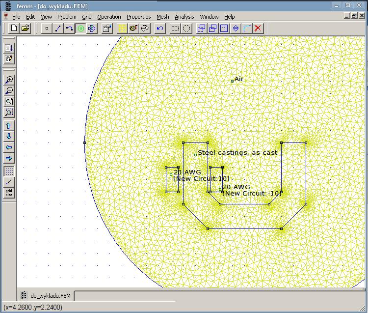
28 The mesh Mesh generator divide modeled area on triangles. Non straight fragments, with a small radius consequently generate a large number of elements. Practical experience shows, that mesh should not exceed elements (but it depends on hardware)

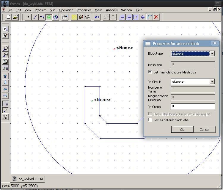
29 The mesh density The number of elements depends on maximal element dimensions. It is possible to declare in material condition of each area. Leaving these value as automatically set, could sometimes not gives reasonable results, but in first tests it is recommended. After some practice, we can try to set the mesh density manually Here, the air gap area is critical

30 The mesh density To set it manually, we have to invoke window with the material (area) property ( properties for selected block ) Unset Let Triangle choose Mesh Size In Mesh size input write correct value

31

32 Calculations After mesh generation, calculations could be started (button with the hand-crank icon). Progress is shown in the special window When the window disappears, calculations are completed and the big magnifying glass icon can be used to display the results in a post-processing window

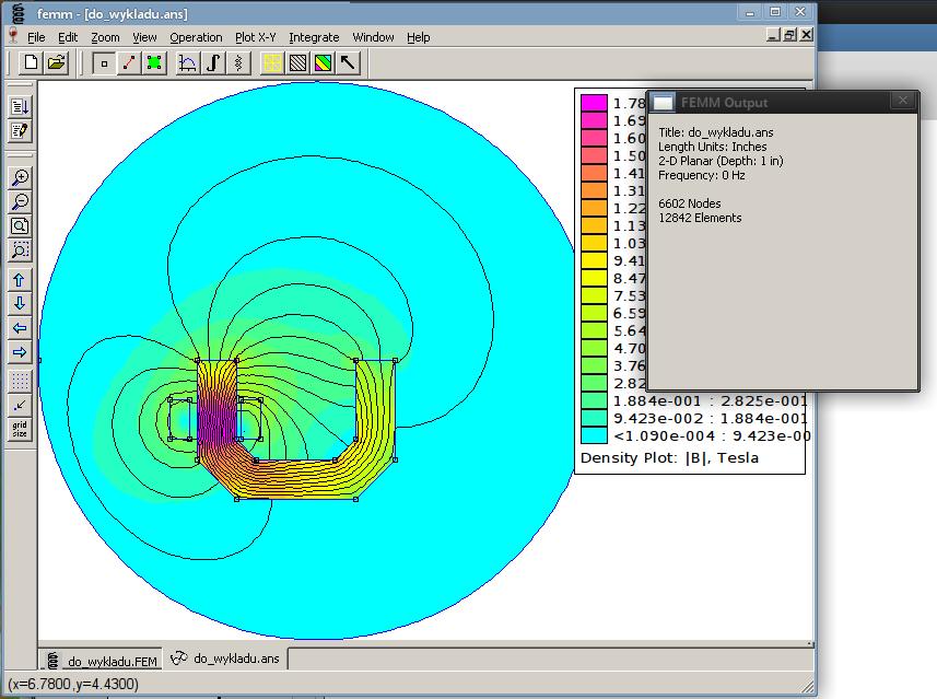
33

34 View the solutions Type of units and way of visualization can be selected from the menu. When we set Show density plot and Show Legend and Show the we get the color map of the plotted value (B or H) Beside, in the window FEMM Output we can find a number of other values in point where the left mouse button was pressed

35 Calculations of forces and etc... When the field is calculated there is a possibility to calculate some values like: forces, flux linkage, inductance, power, etc... For example: if we want to calculate the force acting on some element, we have to ensure that this element is surrounded by air, activate them, and from the integrals menu select Force via...

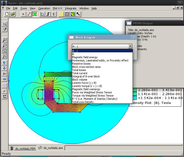
36

37 Inductance, flux linkage... Parameters connected to circuits could be calculated by pressing the button with coil symbol

38

39 Plots There is also possibility to get the plots of some desired values on selected lines Line should be selected by activating the button with red line (section) Then plot can be invoked by the plot button Possible values can be selected in the pop up menu

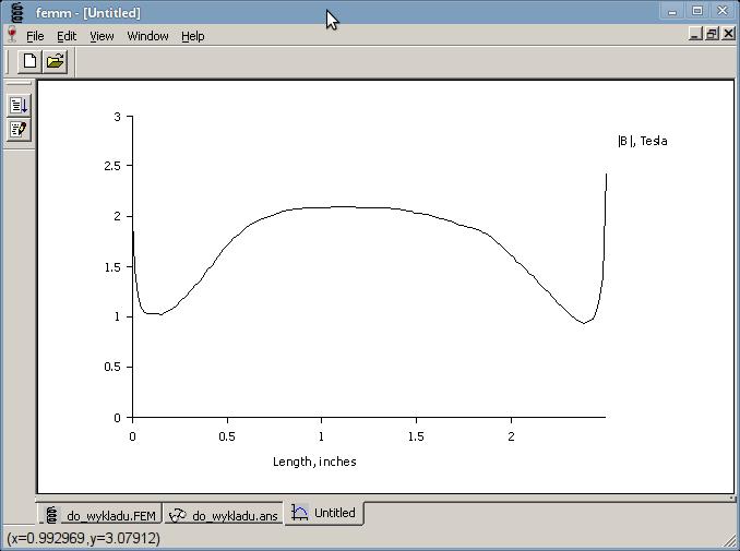
40 Plotting the values

41 Literature Some part are based manual.pdf for FEMM 4.2 program

42 Some informations about the Numerical methods for SGTP - part FEM Two final reports, evaluated, for each person. Contact info: Michał Rad (rad@agh.edu.pl) B1 H20 Informations, materials on Wiki page: home.agh.edu.pl/~rad/wiki/index.php? title=numerical_methods