Interpolation is a basic tool used extensively in tasks such as zooming, shrinking, rotating, and geometric corrections.

Size: px

Start display at page:

Download "Interpolation is a basic tool used extensively in tasks such as zooming, shrinking, rotating, and geometric corrections."

Muriel Lamb
5 years ago
Views:

1 Image Interpolation 48 Interpolation is a basic tool used extensively in tasks such as zooming, shrinking, rotating, and geometric corrections. Fundamentally, interpolation is the process of using known data to estimate values at unknown locations. For example, we want to resize an image of size pixels to pixels. To perform intensity-level assignment for any point in the overlay, we look for its closest pixel in the original image and assign its intensity to the new pixel in the grid. This method is called nearest neighbour interpolation. A more suitable approach is bilinear interpolation, in which we use the four nearest neighbours to estimate the intensity at a given location. Let ( xy, ) denote the coordinates of the location to which we want to assign an intensity value, and let vxy (, ) denote that intensity value. For bilinear interpolation, the assigned value is obtained using the equation vxy (, ) = ax+ by+ cxy+ d, (2.4-6) where the four coefficients are determined from the four equations in four unknowns that can be written using the four nearest neighbours of point ( xy, ). The next level of complexity is bicubic interpolation, which involves the sixteen nearest neighbours of a point: 3 3 i j vxy (, ) = aijxy, (2.4-7) i= 0j= 0

49 where the sixteen coefficients are determined from the sixteen equations in sixteen unknowns that can be written using the sixteen nearest neighbours of point ( xy, ).

2 49 where the sixteen coefficients are determined from the sixteen equations in sixteen unknowns that can be written using the sixteen nearest neighbours of point ( xy, ). Example 2.4: Comparison of interpolation approaches for image shrinking and zooming. It is possible to use more neighbours in interpolation, and there are more complex techniques.

3 2.5 Some Basic Relationships between Pixels 50 Here, we consider some important relationships between pixels in a digital image. Neighbours of a Pixel A pixel p at coordinates ( xy, ) has four horizontal and vertical neighbours: ( x+ 1, y), ( x 1, y), ( xy, + 1), ( xy, 1). This set of pixels is called the 4-neighbuors of p, and denoted by N4( p ). The four diagonal neighbours of p are ( x+ 1, y+ 1), ( x+ 1, y 1), ( x 1, y+ 1), ( x 1, y 1), and are denoted by ND( p ). Adjacency, Connectivity, Regions, and Boundaries Let V be the set of intensity values used to define adjacency. In a binary image, V = { 1} if we are referring to adjacency of pixels with value 1. In a gray-scale image, set V typically contains more elements. For example, with a range of possible intensity values 0 to 255, set V could be any subset of these 256 values. Consider three types of adjacency: (a) 4-adjacency. Two pixels p and q with values from V are 4-adjacency if q is in the set N4( p ).

4 51 (b) (c) 8-adjacency. Two pixels p and q with values from V are 8-adjacency if q is in the set N8( p ). m-adjacency (mixed adjacency). Two pixels p and q with values from V are m -adjacency if (i) q is in the N4( p ), or (ii) q is in the ND( p) and the set N4( p) N4( q) has no pixels whose values are from V. Mixed adjacency is a modified of 8-adjacency. For example, consider the arrangement shown in Figure 2.25 (a) for V = { 1}. The three pixels at the top of Figure 2.25 (b) show ambiguous 8- adjacency, which is removed by using m-adjacency, as shown in Figure 2.25 (c).

5 52 A path from pixel p with coordinates ( xy, ) to pixel q with coordinates ( st, ) is a sequence of distinct pixels with coordinates ( x0, y0), ( x1, y1),, ( xn, yn), where ( x0, y0) = ( xy, ), ( xn, yn) = ( st, ), and pixels ( xi, y i) and ( xi 1, yi 1) are adjacent for 1 i n. n is the length of the path. If ( x0, y0) = ( xn, yn), the path is a closed path. We can define 4-, 8-, or m-paths depending on the type of adjacency. The path shown in Figure 2.25 (b) between the top right and bottom right points are 8-paths, and the path in Figure 2.25 (c) is an m-path. Let S represent a subset of pixels in an image. Two pixels p and q are said to be connected in S if there exists a path between them consisting entirely of pixels ins. If it only has one connected component, set S is called a connected set. Let R be a subset of pixels in an image. We call R a region of the image if R is a connected set. Two regions, R i and R j are said to be adjacent if their union forms a connected set. Regions that are not adjacent are said to be disjoint. The two regions (of 1s) in Figure 2.25 (d) are adjacent only if 8- adjacency is used. Suppose that an image contains K disjoint regions, R k, k= 1,2,..., K, and none of which touches the image border. Let R u denote the union of all the K regions, and let ( R u) c denote its complement. We call all the points in R u the foreground, and all the points in ( R u) c the background of the image.

6 53 The boundary (also called the border or contour) of a regionr is the set of points that are adjacent to points in the complement ofr. Again, we must specify the connectivity being used to define adjacency. For example, the point circled in Figure 2.25 (e) is not a member of the border of the 1-valued region if 4-connectivity is used between the region and its background. As a rule, adjacency between points in a region and its background is defined in terms of 8-adjacency to handle situations like above. The preceding definition is referred to as the inner border of the region to distinguish it from its outer border, which is the corresponding border in the background. This issue is important in the development of border-following algorithms. Such algorithms usually are formulated to follow the outer boundary in order to guarantee that the result will form a closed path. For example, the inner border of the 1-valued region in Figure 2.25 (f) is the region itself. If R happens to be an entire image, then its boundary is defined as the set of pixels in the first and last rows and columns of the image. This extra definition is required because an image has no neighbours beyond its border.

7 Distance Measures 54 For pixelsp, q, and z, with coordinates ( xy, ), ( st, ), and ( vw, ), D is a distance function or metric if (a) Dpq (, ) 0 ( Dpq (, ) = 0 iff p= q ) (b) Dpq (, ) = Dqp (, ), and (c) Dpz (, ) Dpq (, ) + Dqz (, ). The Euclidean distance between p and q is defined as 2 2 [ ] 1/2 De( pq, ) = ( x s) + ( y t). (2.5-1) The D4 distance (called the city-block distance) between p and q is defined as D4( pq, ) = x s + y t. (2.5-2) Example: the pixels with D 4 distance 2 from ( xy, ) form the following contours of constant distance: The pixels with D 4= 1 are the 4-neighbuors of ( xy, ).

8 55 The D8 distance (called the chessboard distance) between p and q is defined as D8( pq, ) = max( x s, y t ). (2.5-3) Example: the pixels with D 8 distance 2 from ( xy, ) form the following contours of constant distance: The pixels with D 8= 1 are the 8-neighbuors of ( xy, ).

9 An Introduction to the Mathematical Tools Used in Digital Image Processing Two principal objectives for this section: (1) to introduce the various mathematical tools we will use in the following chapters; (2) to develop a feel for how these tools are used by applying them to a variety of basic image processing tasks. Array versus Matrix Operations An array operation involving one or more images is carried out on a pixel-by-pixel basis. There are many situations in which operations between images are carried out using matrix theory. Consider the following 2 2 images: a a a a and b b b b The array product of these two images is a a b b a b a b, a21 a = 22 b 21 b 22 a21b21 a22b 22 while the matrix product is given by a a b b a b + a b a b + a b a21 a = 22 b 21 b 22 a21b11 + a22b21 a21b12 + a22b 22 We assume array operations throughout this course, unless stated otherwise.

10 Linear versus Nonlinear Operations 57 One of the most important classifications of an image processing method is whether it is linear or nonlinear. Consider a general operator, H, that produces an output image, gxy (, ), for a given input image, fxy (, ): H[ fxy (, )] = gxy (, ). (2.6-1) H is said to be a linear operator if [ (, ) + (, )] = [ (, )] + [ (, )] H af xy af xy ah f xy ah f xy i i j j i i j j = ag i i( xy, ) + ag j j( xy, ), (2.6-2) where a i, a j, fi( xy, ), and fj( xy, ) are arbitrary constants and images. As indicated in (2.6-2), the output of a linear operation due to the sum of two inputs is the same as performing the operation on the input individually and then summing the results. Example: a nonlinear operation. Consider the following two images for the max operation: f = and f 2 3 = , and we let a 1= 1 and a 2= 1. To test for linearity, we start with the left side of (2.6-2): max (1) + ( 1) = max =

11 Then, we work with the right side: (1)max + ( 1) max = 3 + ( 1)7 = The left and right sides of (2.6-2) are not equal in this case, so we have proved that in general the max operator is nonlinear. Arithmetic Operations The four arithmetic operations, which are array operations, are denoted as sxy (, ) = fxy (, ) + gxy (, ) dxy (, ) = fxy (, ) gxy (, ) pxy (, ) = fxy (, ) gxy (, ) vxy (, ) = fxy (, ) gxy (, ) (2.6-3) Example 2.5: Addition (averaging) of noisy images for noise reduction. Let gxy (, ) denote a corrupted image formed by the addition of noise, η ( xy, ), to a noiseless image fxy (, ): gxy (, ) = fxy (, ) + η( xy, ) (2.6-4) where η ( xy, ) is assumed to be uncorrelated with zero average value. The objective of the following procedure is to reduce the noise content by adding a set of noisy images, { gi( xy, )}. With the above assumption, it can be shown that if an image gxy (, ) is formed by averaging K different noisy images,

12 59 K 1 gxy (, ) = gi( xy, ), (2.6-5) K i = 1 then it follows that E{ gxy (, )} = fxy (, ), (2.6-6) and σ 1 =, (2.6-7) 2 2 g( xy, ) σ ( xy, ) K η where E{ gxy (, )} is the expected value of g, and 2 η( xy, ) 2 g( xy, ) σ and σ are the variances of g and η, all at coordinate ( xy, ). The standard deviation (square root of the variance) at any point in the average image is σ 1 = σ. (2.6-8) gxy (, ) ( xy, ) K η As K increases, (2.6-7) and (2.6-8) indicate that the variability of the pixel values at each location ( xy, ) decreases. This means that gxy (, ) approaches fxy (, ) as the number of noisy images used in the averaging process increases. Figure 2.26 shows results of averaging different number of noisy images to image of Galaxy Pair NGC 3314.

13 60 Example 2.6: Image subtraction for enhancing differences. A frequent application of image subtracting is in the enhancement of differences between images.

Consider image differences of the form gxy (, ) = fxy (, ) hxy (, ). (2.

14 61 As another illustration, we discuss an area of medical imaging called mask mode radiography. Consider image differences of the form gxy (, ) = fxy (, ) hxy (, ). (2.6-9) where (, ) hxy, the mask, is an X-ray image of a region of a patient s body captured by an intensified TV camera located opposite an X-ray source.

Example 2.7: Using image multiplication and division for shading correction. 62 An important application of image multiplication (and division) is shading correction.

15 Example 2.7: Using image multiplication and division for shading correction. 62 An important application of image multiplication (and division) is shading correction. Suppose that an imaging sensor produces images that can be modeled as the product of a perfect image, fxy (, ), times a shading function, hxy (, ): gxy (, ) = fxyhxy (, ) (, ). If hxy (, ) is known, we can obtain fxy (, ) by fxy (, ) = gxy (, )/ hxy (, ). If hxy (, ) is not known, but access to the imaging system is possible, we can obtain an approximation to the shading function by imaging a target of constant intensity. Figure 2.29 shows an example of shading correction.

16 Set and Logical Operations Basic set operations 63 Let A be a set composed of ordered pairs of real numbers. If a= ( a1, a2) is an element of A, then we write a A (2.6-12) Similarly, if a is not an element of A, we write a A (2.6-13) The set with no elements is called the null or empty set and is denoted by the symbol. A set is specified by the contents of two braces: { i. For } example, an expression of the form C= { w w= dd, D} means that set C is the set of elements, w, such that w is formed by multiplying each of the elements of set D by 1. If every element of a set A is also an element of a setb, then A is said to be a subset of B, denoted as A B (2.6-14) The union of two sets A and B, denoted by C= A B (2.6-15) is the set of elements belonging to either A, B, or both.

17 64 Similarly, the intersection of two sets A and B, denoted by D= A B (2.6-16) is the set of elements belonging to both A and B. Two sets A and B are said to be disjoint or mutually exclusive if they have no common elements A B= (2.6-17) The set universe, U, is the set of all elements in a given application. The complement of a seta is the set of elements that are not ina : c A = { w w A} (2.6-18) The difference of two setsa and B, A B, is defined as A B= { w w Aw, B} = A B (2.6-19) c As an example, we would define difference operation: c A in terms of U and the set c A U A =

special coordinates and z denoted intensity.

18 65 Figure 2.31 illustrates the preceding concepts. Example 2.8: Set operations involving image intensities. Let the elements of a gray-scale image be represented by a set A whose elements are triplets of the form( xyz,, ), where x and y are special coordinates and z denoted intensity. We can define the complement of A as the set c A = {( xyk,, z) ( xyz,, ) A}, which denotes the set of pixels of A whose intensities have been subtracted from a constant K. The constant K is equal to 2 k 1, where k is the number of intensity bits used to represent z.

19 66 Let A denote the 8-bit gray-scale image in Figure 2.32 (a). To form the negative of A using set operations, we can form c A = A = {( xy,,255 z) ( xyz,, ) A} n This image is shown in Figure 2.32 (b). The union of two gray-scale set A and B may be defined as the set A B= { max( ab, ) a Ab, B} z For example, assume A represents the image in Figure 2.32 (a), and let B denote an array of the same size as A, but in which all values of z are equal to 3 times the mean intensity, m, of the elements of A. Figure 2.32 (c) shows the result.

Logical operations 67 When dealing with binary images, it is common practice to refer to union, intersection, and complement as the OR, AND, and NOT

33 shows the result of operation that the set of foreground pixels belonging to A but not tob, which is the definition of set difference in A B= { w w

20 Logical operations 67 When dealing with binary images, it is common practice to refer to union, intersection, and complement as the OR, AND, and NOT logical operations. Figure 2.33 illustrates some logical operations. The fourth row of Figure 2.33 shows the result of operation that the set of foreground pixels belonging to A but not tob, which is the definition of set difference in A B= { w w Aw, B} = A B (2.6-19) The last row shows the XOR (exclusive OR) operation, which is the set of foreground pixels belonging to A or B, but not both. The three operators, OR, AND, and NOT, are functionally complete. c

21 Spatial Operators 68 Spatial operations are performed directly on the pixels of a given image. Single-pixel operations This is the simplest operation we perform on a digital image to alter the values of its individual pixels based on their intensity: s= Tz ( ) (2.6-20) where T is a transformation function, z is the intensity of a pixel in the original image, and s is the intensity of the corresponding pixel in the processed image. Neighbourhood operations Let S xy denote the set of coordinates of a neighbourhood centered on an arbitrary point ( xy, ) in an image, f. Neighbourhood processing generates a corresponding pixel at the same coordinates in an output image, g. The value of that pixel is determined by a specified operation involving the pixels ins xy.

22 69 Figure 2.35 shows a process performed in a neighbourhood of size m n, which can be expressed in equation form: 1 gxy (, ) = frc (, ) mn (2.6-21) ( rc, ) S xy where r and c are the row and column coordinates of the pixels whose coordinates are numbers of the set S xy.

23 Geometric spatial transformations and image registration 70 Geometric transformations modify the spatial relationship between pixels in an image. A geometric transformation consists of two basic operations: (1) a spatial transformation of coordinates, and (2) intensity interpolation that assigns intensity value to the spatially transformed pixels. The transformation of coordinates may be expressed as ( xy, ) = T{ ( vw, )} (2.6-22) where ( vw, ) are pixel coordinates in the original image and ( xy, ) are the corresponding pixel coordinates in the transformed image. For example, the transformation ( xy, ) = T{ ( vw, )} = ( v /2, w /2) shrinks the original image to half. One of the most commonly used spatial coordinate transform is the affine transform, which has the general form t 11 t12 0 xy 1 = vw 1 T= vw 1 t21 t22 0 t31 t32 1 [ ] [ ] [ ] (2.6-23) This transformation can scale, rotate, translate, or shear a set of coordinate points, depending on the value chosen for the elements of matrix T.

24 71 Table 2.2 illustrates the matrix values used to implement these transformations. In practice, we can use (2.6-23) in two basic ways. Forward mapping It consists of scanning the pixels of the input image and, at each location, ( vw, ), computing the spatial location, ( xy, ), of the corresponding pixel in the output image using (2.6-23) directly.

72 A problem with the forward mapping approach is that two or more pixels in the input image can be transformed to the same location in the output image.

25 72 A problem with the forward mapping approach is that two or more pixels in the input image can be transformed to the same location in the output image. It is also possible that some output locations may not be assigned a pixel at all. Inverse mapping It scans the output pixel locations and, at each location,( xy, ), computes the corresponding location in the input image using 1 ( vw, ) = T ( xy, ) It then interpolates among the nearest input pixels to determine the intensity of the output pixel value. Example 2.9: Image rotation and intensity interpolation. Image registration is an important application of digital image processing used to align two or more images of the same scene. In image registration, we have the input and output images, but the specific transformation that produced the output image from the input generally is unknown. We need to estimate the transformation function and then use it to register the two images.

26 73 For example, it may be interest to align (register) two or more images taken at approximately the same time, but using different imaging systems. Or, the images were taken at different times using the same instrument. One of the principal approaches is to use tie points (control points), which are corresponding points whose locations are known precisely in the input and reference images (the images against which we want to register the input). There are numerous ways to select tie points, ranging from interactively selecting them to applying algorithms that attempt to detect these points automatically. The problem of estimating the transformation function is one of modeling. Suppose that we have a set of four tie points each in an input and a reference image. A simple model based on a bilinear approximation is given by and x= cv 1 + cw 2 + cvw 3 + c4 (2.6-24) y= cv 5 + cw 6 + cvw 7 + c8 (2.6-25) During the estimation phase, ( vw, ) and ( xy, ) are the coordinates of tie points in the input and reference images. Once we have the coefficients, (2.6-24) and (2.6-25) become our vehicle for transforming all the pixels in the input image to generate the desired new image. If the tie points were selected correctly, the new image should be registered with the reference image.

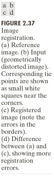
27 74 Example 2.10: Image registration.

Image Transforms 75 In some cases, image processing tasks are best formulated by transforming the input images, carrying the specified task in a transform domain, and applying the inverse transform

28 Image Transforms 75 In some cases, image processing tasks are best formulated by transforming the input images, carrying the specified task in a transform domain, and applying the inverse transform to return to the spatial domain. A particularly important class of 2-D linear transforms, denoted by (, ) Tuv, can be expressed in the general form M 1N 1 Tuv (, ) = fxyrxyuv (, ) (,,, ) (2.6-30) x= 0y= 0 where fxy (, ) is the input image, and rxyuv (,,, ) is called the forward transformation kernel. Variable u and v are called the transform variables. Given Tuv (, ), we can recover fxy (, ) using the inverse transform of Tuv (, ) M 1N 1 fxy (, ) = Tuvsxyuv (, ) (,,, ) (2.6-31) u= 0v= 0 where sxyuv (,,, ) is called the inverse transformation kernel. Together, (2.6-30) and (2.6-31) are called a transform pair.

29 76 Example 2.11: Image processing in the transform domain. The forward transformation kernel is said to be separable if rxyuv (,,, ) r ( xur, ) ( yv, ) = 1 2 (2.6-32) The kernel is said to be symmetric if r1( xy, ) is functionally equal to r2( xy, ), so that rxyuv (,,, ) r ( xur, ) ( yv, ) = 1 1. (2.6-33)

EC-433 Digital Image Processing

EC-433 Digital Image Processing Lecture 4 Digital Image Fundamentals Dr. Arslan Shaukat Acknowledgement: Lecture slides material from Dr. Rehan Hafiz, Gonzalez and Woods Interpolation Required in image