Curvature Adjusted Parameterization of Curves

Transcription

1 Purdue University Purdue e-pubs Department of Computer Science Technical Reports Department of Computer Science 1989 Curvature Adjusted Parameterization of Curves Richard R. Patterson Chanderjit Bajaj Report Number: Patterson, Richard R. and Bajaj, Chanderjit, "Curvature Adjusted Parameterization of Curves" (1989). Department of Computer Science Technical Reports. Paper This document has been made available through Purdue e-pubs, a service of the Purdue University Libraries. Please contact epubs@purdue.edu for additional information.

2 CURVATURE ADJUSTED PARAMETERIZATIONS OF CURVES Richard R. Patterson Indiana University-Purdue University Indianapolis, IN and Chanderjit Bajaj* Computer Sciences Department Purdue University Technical Report CSD-TR-907 CAPO Report CER September, 1989 * Supponcd in part by ARO ContracL DAAG29 8S-e0018, NSF grant DMS and ONR conlracl NOOO14 88-K-0402.

3 Curvature Adjusted Parametrizations of Curves Richard R. Patterson and Chanderjit Bajaj Indiana University - Purdue University at Indianapolis and Purdue University July 21,1989 One way of graphing a curve in the plane or in space is to use a parametrization X(t) = (x(t), yet)) or X(t) = (x(t), yet), z(t)), a:s; t:s; b. We compute X as t is advanced by small steps tlt and connect the cm-responding points by line segments, getting a piecewise-linear approximation to the curve. A given curve can have many different parametrizations, and some are better than others for the purpose of graphing. In particular we might say a parametrization of a curve is good if with a constant value b..t the points on the curve tend to bunch up in regions of high curvature and spread. out in regions of low curvature. In this paper we define an ideal curvature parametrization for plane curves and three possible extensions to space curves. "Vole show how the idea leads to a useful step adjustment function for b..t and compare it to other step adjustment methods. ARC-LENGTH PARAMETRIZATION We begin by reviewing the definition of the arc-length parametrization. Suppose we are given a curve with a smooth parametrization X(t), a.$ t ~ h, for which the length of the tangent vector IX'(t)1 does not vanish. The arc-length is defined by set) = l' IX'(u)ldu. Let L = s(b) be the length. We have s'(t) = IX'CI)I. Although we cannot usually find the 1

4 inverse function t(s) explicitly, it exists since s(t) is increasing, and dt 1 ds IX'I If we reparametrize the curve In terms of s, then X(s), 0 < s < L, IS the arc-length parametrizat1.on. We see that dx dx dt X'(t) -=--= =t ds dt ds IX'(t)1 where t is the unit tangent vector. If we plot X(s) for values of s incremented by a constant step 6.s and form the corresponding polygonal curve,...ve obtain a piece'''ise linear approximation to the curve by a polygon whose sides all have approximately the same length but which generally does not hug the curve closely at sharp bends. CURVATURE PARAMETRIZATION FOR PLANE CURVES At a point of a plane curve, let r./> be the angle between t and the horizontal (see Figure 1). Unless the curve is vertical at the point, tan r./> = y'ix'. The curvature at this point is defined by K. = dr./>ids. We see that K. is positive if the curve is bending to the left, negative if it is bending to the right, and zero at an inflection point. In a region in which K. is nonzero we can use r./> as a parameter for X. We call X(r./» the CUT1Jature parametrization. In the curvature parametrization the derivative vector is given by dx dxds 1 -=--=-t. d ds d K If we graph X using constant step 6.r./>, the points of the curve will tend to bunch up in regions of high curvature. Just as with the arc-length parametrization it is not usually possible to find the curvature parametrization explicitly. Nevertheless we can use the ideas to obtain a simple method to adjust the original steps f:j,t to come closer to the ideal situation. As usual in differential geometry, everything is deduced using the chain rule. Because d = d ds = IX'I dt dsdt K., 2

5 we have I dt =,!X'! d. In order to cancel out the sign of the curvature we take the absolute value and use I for a step adjustment function. Even though we may not be able to get the curvature parametrization explicitly we can use a constant step f::1 and use the step adjustment fundon to get a fit st order approximation by which to adjust the step f::1t : Both", and IX I! are easy to find.as functions of t:!x'! = (x'(t)' + y'(t)')l/' x'(t)yu(t) - y'(t)xu(t),- - (x'(i)' + y'(i)')3/2 so that X' X' dt = IX', XU] d, where Thus the step adjustment function is l X' XU] = Ix' ' x" y" y'. IX' X'! IX', XU] At an inflection point, '" = 0 and the step adjustment function becomes infinite. Thus I to be practical, a program needs an upper bound on f::1t. Example 1. Consider the parabola y = x 2, parametrized by XCt) = (t,t 2 ). From X/(t) = (1, 2t), we see tan = 2t, t = ~ tan. 'VI'e can find the curvature parametrization explictly in this case: I X( ) = 4Ian (2,lan ). 3

6 We can also compute X'. X' = 1 + 4t 2 = sec 2 r/j, 2 ~ = (1 + 4t')'/' = 2cos' 1>, and XI X' 1 1 dt= [X',X"ld1>= 2(1 +4t')d1> = 2 sec '1>d1>. The step adjustment function is t'. 2 Example 2. In the case of the ellipse pa.rametrized by X(t) = (acost,bsint) we ha.ve X'(t) = (-asint,bcost) so Computing tanr/j = b --cott. a and ab K = o(-a';;-csic"n"-:t-+'::::b''--co-s""''-:t"'')'''/'''' we find the step adjustment function a 2 sin 2 t + b 2 cos 2 t ab Figure 2 shows an ellipse drawn first with fixed step b..t, second using this formula and a fixed step 6.r/J! and finally using a fixed step 6. with an upper bound on 6.t. Qnly the points are plotted to make the spacing easier to see. 4

7 Example 3. The circle x 2 + y2 = T 2 has the rational parametrization T - Tt 2 2rt X(t) = ( 1 +t' ' 1 + t') This parametrization is useful for graphing an arc of a circle, -k.::; t.::; k, but not the entire circle since the point with coordinates (-7',0) corresponds to t = ±co. Figure 3 illustrates an arc drawn first with fixed step b..t and then again using the step adj ustment function t + ~t2. In this example 'we are correcting to get the effect of the trigonometric parametrization (r cos 0, r sin B), which is a naturally occuring curvature parametrjzation. In each of the examples above it is possible to solve the differential equation dt X'-X' d [X', X"] to get t explicitly as a function of,p. In general if we require more than the first order approximation given by the step adjustment function the differential equation can be solved numerically; see Mastin [1]. The step adjustment method used by the authors of the computer algebra program Scratchpad employ a step adjustment method which does not require prior knowledge of the curve to be graphed. They begin with a fixed step and subdivide it if either the next segment is too long or fontis too great an angle with the previous segment [2]. SPACE CURVES Space curves have both curvature and torsion. There are at least three possible extensions of the step adjustment function which depend on the angle we choose to play the role of,p. The first corrects for curvature, the second for torsion, and the third for both. Let,pI be the angle between t(a) and t(s). The curvature of the space curve is defined by #,.. K::::-::::t t ds ' 5

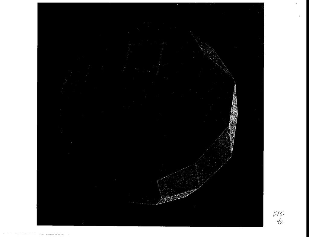
8 where the dot indicates the derivative with respect to arc length s. Using d, dt d, ds ds dt' we obtain a step adjustment function that corrects for CUl"Vature: The binormal vector b is defined by 1 dt = -1-1d,. Ii X' X' x Xu b ~ "IX"";-x~X;-;''''I It is a unit vector perpendicular to the tangent vector and exists at points where Xl x X" is not the zero vector. Let 2 be the angle beh..'een b(a) and b(t). The torsion of the space curve is defined by d,.. T = ds = b b. A second step adjustment function that corrects for torsion is derived in a similar way as the first 1 dt = TIX'I d,. The Frenet frame at a point of the curve is completed by the principal normal vector p = b X t. Let 4Ja be the angle formed between pea) and pet). The third curvature of the curve is defined by using the Frenet formulas [3]. The third step adjustment function corrects for both curvature and torsion dt = 1.j~' + T'IX'l d 3. Example 4. parametrization In analogy with example 3 a patch of the unit sphere has the rational 1_s 2 _t 2 x(s,t) = l+s' +t' 6

9 for -k.$ Sit.$ k. 28 y(s,t) = l+s'+t' 2t z(s, t) = 1 ', +8 +t The coordinate curves on this surface are planar, so their torsion is zero. Figure 4 shows a spherical patch graphed with constant steps 6.s,.6..t and again after the correction for curvature. Which of these three methods is preferable to use when manufacturing an object on which one of these curves lies needs more investigation. If the final goal is a projected two-dimensional image of the curve then it is more reasonable to project the curve first and use the planar step adjustment method on the image curve. This is because no step adjustment of the space curve will always appear to give the correct steps when the curve is viewed from any arbitrary angle. REFERENCES 1. C. W. Mastin, "Parameterization in Grid Generation," Computer-aided Design, Vol. 18, 1986, pp C. Williamson, private communication. 3. E. Kreyszig, Differential Geometry, University of Toronto Press, Toronto, ACKNOWLEDGEMENTS The research for this paper was supported in part by ARO Contract DAAG29-85 C0018 under Cornell MS1, NSF grant DMS , ONR Contract N K-0402 and a grant from the Chrysler Corporation to IUPUI. 7

10 Captions for figures Figure 1. Defining the curvature 6.1. Figure 2. An ellipse drawn using (a) fixed 6.1, (b) fixed 6.~, (c) fixed 6.~ with bounded Figure 3. A circular arc drawn using (a) fixed.6.t, (b) fixed 6 J. FigUl-e 4. A spherical patch drawn with (a) fixed.6.t and.6.s, (b) correction for curvature. In each direction 40 steps were used in both cases. 8

11 X (b) t X (a) x

12 ..:( ",'-.

13 '-'

14 '-!... '-'

15 ... ',.A

16 fig ;: (3

17

18 F/ct/b