Exercise 5. Height above Nearest Drainage Flood Inundation Analysis

Transcription

1 Exercise 5. Height above Nearest Drainage Flood Inundation Analysis GIS in Water Resources, Fall 2018 Prepared by David G Tarboton Purpose The purpose of this exercise is to learn how to calculation the height above the nearest drainage (HAND) from a digital elevation model, to use this HAND raster to derive stream reach hydraulic properties, flood inundation depth and a flood inundation map. Computer and Data Requirements To carry out this exercise, you need to have a computer which runs ArcGIS Pro Version 2.0 or higher. The following data is provided in Ex5Data.zip ( OnionHand.gdb. A geodatabase containing NHDPlus flowlines and catchments for Onion Creek. This also contains address points that will be used in assessing addresses vulnerable to flooding. These have been projected to a UTM zone 14 coordinate system for consistency. Onion3.tif. A 10 m digital elevation model from the National Elevation dataset. This DEM was obtained from the National Map, extracted to a 2 km buffer around the watershed and projected to the same UTM zone 14 coordinate system as the vector data, for consistency. It has also had a flow direction conditioning procedure applied to it using TauDEM to remove barriers along high resolution NHD flowlines. As you do this exercise, you are going to create additional feature classes and rasters stored as.tif files. You can create a new geodatabase for the exercise and put the new feature classes into that, or store them in the utm14 feature dataset shown above. You will store all the new.tif files in the folder for Exercise 5 alongside the Onion3.tif. From time to time you will shift back and forth between these two data storage locations 1

2 Computation of Height above the Nearest Drainage Raster 1. Preparing the inputs Unzip the zip file and add the DEM and NHDFlowlines and Catchments to a Map in ArcGIS Pro. To evaluate the height above the nearest neighbor raster we need a raster of stream grid cells consistent with NHDplus. While it is possible to directly convert the NHDFlowline dataset to a raster, it is preferable to have a stream raster consistent with DEM flow directions. We therefore use a procedure to identify dangling vertices of the NHD flowlines and use these as seed points to delineate a stream raster. Dangling vertices are points at the extreme "dangling" ends of a feature class. Open the geoprocessing panel and search for "dangle", then select the Feature Vertices to Points tool. Set the parameters as follows. 2

3 Add the output Feature Class DanglingVertices in the OnionHand.gdb Geographic feature class and run the tool. You should see a map with points at the end of each stream. Next we need to convert these points to a raster to use in seeding the stream network delineation. Locate the Feature to Raster Geoprocessing tool and set the following inputs. Set the field to StartFlag. This is a convenient field in the attribute table that has the value of 1. Save the output raster "Start.tif" in the same location as the DEM. I used the Ex5 folder. Do not press Run just yet. Click on Environments. Then for Output Coordinate System click on Onion3.tif. 3

4 The display will switch to NAD_1983_UTM_Zone_14N indicating that this coordinate system from the Onion3.tif file will be used. This is important to get the resulting raster the same dimensions as the DEM. Next click on Extent and Snap Raster and in both cases pick Onion3.tif. Lastly click on Cell Size and again choose Same as layer Onion3.tif. These settings are all necessary so that the resulting Start.tif raster that is produced has the same dimensions (columns, rows, cell size, coordinate system, etc.) as the Onion3.tif DEM. The environments parameter settings should be as follows. Then click run. 4

5 The result should be a new raster "start.tif" that has the same number of rows and columns as Onion3.tif DEM. Check this, as if this is not the case the stream delineation will not work. If you open the Attribute Table for Start.tif you will see there are 42 grid cells with the value of 1 and one with a grid value of 0. This is the single cell near the outlet. There are many more grid cells overall (7274 * 3170). The way we are going to use this raster requires non-nodata values everywhere, so let s reclassify nodata values to 0. Locate the Reclassify (Spatial Analyst) Geoprocessing tool. Set the input raster as Start.tif and adjust the values as follows. Save the output as Startrc.tif (rc for reclassified) and Run. The result should be a raster with values 0 and 1, with no data values. If you zoom in over the sources of NHDFlowlines you will see that there is a single cell with a value of 1 at the source of each stream. The 5

6 raster Startrc.tif will be used together with Onion3.tif to delineate a stream raster using the procedures used in Exercise DEM derived stream network and Height Above the Nearest Drainage (HAND) The sequence of steps give below uses tools from the Hydrology Toolbox to compute a stream raster from the flow direction conditioned DEM provided and then calculate HAND for this stream raster. To visualize the process as you work, create a 10 m contour layer for the Onion3.tif DEM and arrange your map to show contours, the Watershed outline (which you may need to add), Streamrc.tif start cells and NHDFlowline streams. Use the procedure shown in Exercise 3, p.37 if you don t remember how to create contours. Zoom in on an area of interest to see the raster start cell at the beginning of each NHDFlowline stream 6

7 The steps are: 1. Fill to remove sinks and hydrologically condition the DEM. 2. Flow direction with the D8 option. D8 is used for stream delineation. 3. Flow Accumulation with Startrc as weight raster. 4. Create stream raster. Use Con tool to create stream raster from grid cells with weighted flow accumulation greater than or equal to Flow direction with the DINF option. Dinfinity is used for HAND to average over multiple flow paths. 6. Flow distance with the DINF flow direction and vertical distance. This produces HAND. 7. Stream link. This is used to produce the DEM derived stream network. 8. Watershed. This is used to produce the DEM derived catchments. 9. Stream to Feature. This is used to produce the vector feature class of the DEM derived stream network. 10. Calculate the catchment polygon layer using Raster to Polygon Following are the inputs you should use for each of these steps Fill 7

8 Flow Direction with D8 Option Note that D8 is used for stream delineation because we do not want to map streams as diverging or spreading out, so need a flow direction representation that has flow going to only one downslope grid cell. Flow Accumulation with Startrc as weight raster You should see a result like the following 8

9 Here I symbolized 0 values as no color. Note the flow accumulation path starting from each grid cell but tracing down the DEM valley, that is not perfectly aligned with the NHDFlowline. This is because we are using a 10 m resolution DEM and the NHDFlowline was mapped at "medium resolution" nominally 1: scale. Create stream raster Use Con tool to create stream raster from grid cells with weighted flow accumulation greater than or equal to 1. 9

10 This stream raster will be used as the target for HAND. Flow direction with the DINF option Note that Dinfinity is used for HAND because we are going to be calculating distances to streams across hillslopes. Dinfinity is generally better for representing smooth hillslope flow fields, whereas D8 is used in valleys where the topography is convergent and we do not want dispersion of flow. Note also that the output drop raster is saved as "Onion3pslp.tif" as it represents percentage slope that we will use later to compute bed area. Flow distance with the DINF flow direction and vertical distance 10

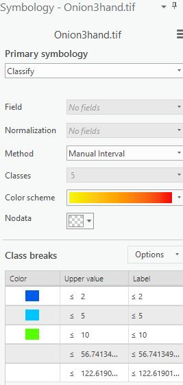
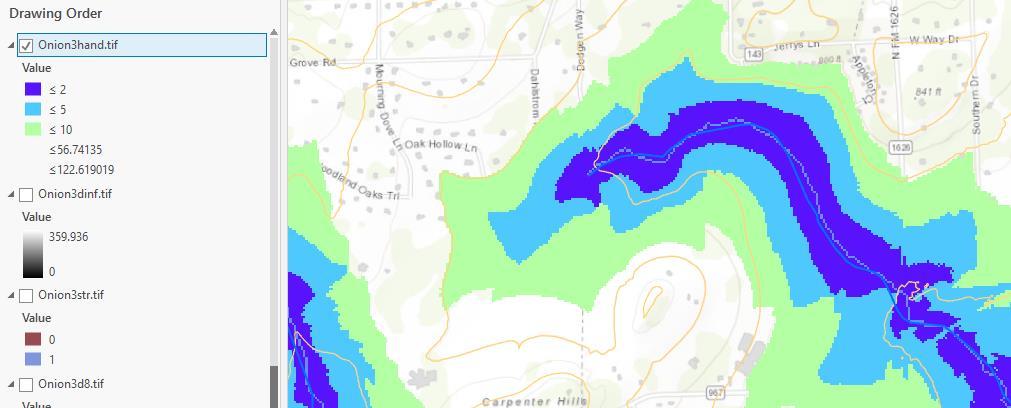
11 The result from this step is Height above the Nearest Drainage or HAND. Examine a few grid cell values to see that this is 0 on mapped streams and increases as you move away from streams. In the below I have symbolized HAND using the Classify option to show grid cells with values less that 2 m, 5 m and 10 m above the stream. Use 5 classes and manually set the upper limit of the first three classes to be 2, 5, 10, respectively and manually choose the colors to be associated with these classes. Put No Color for the two remaining classes with higher HAND values. 11

12 12

13 To turn in. Make a map layout of the HAND raster that illustrates it nicely. Include NHDFlowline and DEM contour feature classes in this map, together with a legend, title and scale bar. Include a map frame that depicts the full watershed extent as well as a frame that is zoomed in to an area of interest (of your choosing) to illustrate detail. Stream link The result is a raster layer where each stream reach has a unique identifier in the grid value. Watershed The result is a raster layer where grid cells belonging to the catchments draining to each stream reach (in Onion3lnk.tif) get the same grid value as the link to which they drain, providing the identifier linking catchments to streams. 13

14 Stream to Feature The result, "drainageline" is a feature class with the DEM derived stream network. In doing the above be sure to uncheck Simplify polylines so that the streams delineated go through grid cell centers exactly and are not approximated. Store the drainageline feature in the same location as you earlier stored the dangling vertices. Calculate the catchment polygon layer using Raster to Polygon Be careful to choose the options as shown: not to Simply polygons and to create multipart features. The result is "Catchpoly", a catchment polygon feature class that was derived from the DEM. Note that this does not align perfectly with the NHDPlus catchments, in the "Catchment" feature class provided, again because of the difference in precision of the DEM used. 14

15 In the illustration below some differences between NHD catchments (green borders) and DEM derived catchment polygons can be seen, as well as differences between the NHDFlowline streams (blue) and DEM derived streams (red). There are also locations where NHDFlowlines are segmented along a single stream reach inbetween junctions. As a result there are fewer DEM derived catchments than NHDPlus catchments. The red circle above illustrates one case of this. Following is an illustration of HAND where the difference between DEM derived network (red) and NHDFlowline network (blue) is evident, and you can see that HAND was computed to the DEM derived network. 15

16 To turn in. Make a map layout that illustrates an example of where the DEM derived stream network and NHDPlus flow network differ, and how HAND has been calculated based on the DEM derived network similar to the illustration above. Write a few sentences that describe and explain your illustration. 3. Hydraulic Properties Now lets determine hydraulic properties and potential flooding for one particular catchment. Lets pick FeatureID= This was one that was particularly affected by flooding a few years ago. Open the attribute table of Catchments. Click on Select by attributes and add a clause FEATUREID is Equal to and Run. You should see a specific NHD plus catchment selected. Zoom to Selection to see it better. 16

17 Note that the feature selected above is from the Catchment Feature Class. Identify the corresponding catchment delineated from the DEM in the Catchpoly layer. To do this turn on the Catchpoly layer and turn off the Catchment layer. Configure the Explore button to select from "Selected in Contents", click on Catchpoly in contents then click the select button and select within the area of the initially selected polygon. 17

18 You should see the following polygon in Catchpoly selected 18

19 Note that this is different from the Catchment polygon selected earlier. This is the area that, according to the DEM drains directly to the stream reach indicated above. It should be used in the calculation of hydraulic properties for this reach, rather than the polygon defined by Catchment because Catchment includes area where HAND has been evaluated draining to a different stream. Specifically, in the illustration below the area circled in red is part of Catchment , but according to the DEM drains to the stream reach to the left, not the stream reach associated with Catchment

20 This imperfect alignment between DEM delineated catchments and NHDPlus catchments is one of the challenges in using NHDPlus catchments with the HAND method and is the subject of research to better partition stream reaches and their associated areas. It is also motivating the USGS to consider raster elevation data and vector hydrography data development in an integrated project, referred to as EleHydro to reduce these sort of inconsistencies between data derived differently. With the Catchpoly polygon identified above selected export it to your project geodatabase as a feature class named CatchPolySelect. Locate the Geoprocessing tool Extract by Mask. Set the input raster as Onion3hand.tif, input feature mask data as CatchPolySelect, and output raster as CatchHand.tif. I put this in the "Ex5" folder. Click Run. Note that this function extracts the HAND raster for only the CatchPolySelect feature class. 20

21 This results in a raster with values retained (masked out) just for the selected polygon. This allows us to examine the HAND layer for this polygon in detail. Perform the following raster calculations 21

22 lt1.tif is a raster with all grid cells less than 1 m. If you look at it's attribute table you will see that there are 658 grid cells with a value less than 1. If you look at its Raster Information in properties you will see that the cell size is 10 m. The area is thus 100 m 2 22

23 The surface area at a stage of 1 m is thus 658 x 100 = m 2. d1.tif is a raster with grid cells that give inundation depth for a stage height of 1 m. Look at its Statistics in Properties to see its mean value. This mean depth of m represents a volume of V = = m 3 To obtain the wetted bed area we need a slope raster. Use Onion3pslp.tif from the DINF flow direction calculation as the slope of each grid cell. Evaluate the following Raster Calculator expression This evaluates for each grid cell 1 + slp 2. By dividing by lt1.tif only grid cells within the area with stage less than 1 are evaluated. Statistics on this indicate a mean of

24 The following formula gives bed area A b = A c 1 + slp 2 Here this is 658 x 100 x = m 2 Use identify to determine the length of the drainageline segment through this catchment (length = 4308 m). Use identify on Onion3fel.tif at the end points of this drainage line to obtain the drop in elevation (z1= , z2= ), and calculate bed slope S o=(z2-z1)/l = Assume mannings n = With this information the hydraulic properties and uniform flow discharge needed for a rating curve can be calculated. Stage h (m) stage (ft) cell size(m 2 ) flooding cell num 658 sb A s (m 2 ) A b (m 2 ) Inundation depth (m) V (m 3 ) L (m) z1 (m) z2 (m) A = V/L (m 2 ) 10.9 P=A b/l (m) R=A/P (m) S n Q = 1 1 n AR2 2 3S o (m 3 /s) 7 Q (ft 3 /s) = Q (m 3 /s) x Follow the procedure above to determine the discharge associated with stage heights of 6, 10 and 14 m and fill in the table above. 24

25 To turn in. Table giving hydraulic properties and discharge associated with stage heights of 6, 10 and 14 m. Plot a rating curve with discharge on the x axis and stage height on the y axis (convert to ft) that has four points corresponding to depths of 1, 6, 10 and 14 m. The NHDFlowline feature class provided for this exercise has an attribute FloodFlow_cfs. This is the last column. This was calculated taking the October 31, 2013 Onion Creek flood discharge of 120,000 ft 3 /s and scaling by Q00001A to obtain an estimate that is roughly based on contributing area for each reach. The FloodFlow_cfs for this reach is indicated as ft 3 /s. Interpolate based on the results above a stage height that corresponds to this discharge. If you are unable to succeed with the calculations above pick a stage height of 6 m. To turn in. Report the stage associated with a potential flood discharge of ft 3 /s in this catchment. 4. Inundation and Impact Use Raster Calculator functions to determine the Inundation depth in this catchment for the stage height you calculated. Add the AddressPt Feature class to your map. Use Select by Location to Create a new feature class that is just address points in CatchPolySelect. 25

26 You should see the following with just address points in CatchPolySelect selected. 26

27 Export the selected AddressPt dataset as a feature class AddressPtSelect. 27

28 Use Extract Values to Points to determine HAND from CatchHand.tif for addresses in this catchment. What you are doing is to overlay the AddressPts on the HAND raster and determine for each AddressPt what the HAND value is for that Address location. Open the attribute table for HandPt. RASTERVU gives the raster value (HAND) for each address point. Sort Ascending on the RASTERVU column. You will see that the water depth in Onion Creek has to rise to about 8m before many address points start getting flooded in this area. 28

29 Select all address points with RASTERVU less thanthe flood stage height you determined to show the addresses subject to flooding for this discharge. Following are address points with HAND value less than 9 m. 29

30 Note that some of these address points are incorrect and not adjacent to the stream. This occurs due to inconsistencies between the delineation of CatchPoly.tif using D8 and HAND calculated using DINF, where part of the HAND value seems to be based on Marble Creek to the east. For the purposes of this exercise, ignore these discrepancies. Prepare a map that shows addresses where the HAND value is less than the flood stage height you determined. These are addresses subject to flooding for this discharge. Prepare a plot that shows the distribution of inundation depths (as a histogram) for address points within this catchment. To turn in. A layout showing the catchment from CatchPoly that you used for this HAND analysis. On this layout include HAND, potential flood inundation depth based on your calculate flood stage. Include address points using a separate symbol for address points subject to flooding in this potential flood. Include your plot that shows the distribution of inundation depths for address points potentially subject to flooding in this catchment at this discharge. OK. You are done! Summary of Items to turn in. 1. Make a map layout of the HAND raster that illustrates it nicely. Include NHDFlowline and DEM contour feature classes in this map, together with a legend, title and scale bar. Include a map frame that depicts the full watershed extent as well as a frame that is zoomed in to an area of interest (of your choosing) to illustrate detail. 2. Make a map layout that illustrates an example of where the DEM derived stream network and NHDPlus flow network differ, and how HAND has been calculated based on the DEM derived network similar to the illustration above. Write a few sentences that describe and explain your illustration. 3. Table giving hydraulic properties and discharge associated with stage heights of 6, 10 and 14 m. Plot a rating curve with discharge on the x axis and stage height on the y axis (convert to ft) that has four points corresponding to depths of 1, 6, 10 and 14 m. 4. Report the stage associated with a potential flood discharge of ft 3 /s in this catchment. 5. A layout showing the catchment from CatchPoly that you used for this HAND analysis. On this layout include HAND, potential flood inundation depth based on your calculate flood stage. Include address points using a separate symbol for address points subject to flooding in this potential flood. Include your plot that shows the distribution of inundation depths for address points potentially subject to flooding in this catchment at this discharge. 30