Northern California Fault System LiDAR Survey. (March 21 April 17, 2007) Processing Report

Transcription

1 Northern California Fault System LiDAR Survey (March 21 April 17, 2007) Processing Report

2 Tables of Content 1. LIDAR SYSTEM DESCRIPTION AND SPECIFICATIONS NOCAL FIELD CAMPAIGN SURVEY PLANNING PARAMETERS GPS DATA PROCESSING IMU DATA PROCESSING LASER POINT PROCESSING OVERVIEW CLASSIFICATION DEM PRODUCTION SPECIAL NOTE ON THE NOCAL LIDAR DATA GEOREFERENCING FILE FORMATS AND NAMING CONVENTIONS...23 APPENDIX A NOCAL SURVEY FLIGHT DAYS OVERVIEW SURVEY PARAMETERS LIST OF OSU NAVIGATION SOLUTION VERSIONS USED FOR NOCAL PROCESSING DASHMAP PROCESSING PARAMETERS

3 1. LiDAR System Description and Specifications This survey used an Optech Gemini Airborne Laser Terrain Mapper (ALTM) serial number 06SEN195 mounted in a twin-engine Cessna Skymaster (Tail Number N337P). This ALTM was delivered to the UF in March, 2007 as the first of its kind in the United States, and the NoCal project was the first project surveyed with this system. System specifications appear below in Table 1. Operating Altitude Horizontal Accuracy Elevation Accuracy Range Capture Intensity Capture m 1/11,000 x altitude; ±1-sigma 5-10 cm typical; ±1-sigma Up to 4 range measurements per pulse, including last 4 Intensity readings with 12-bit dynamic range for each measurement Variable from 0 to 25 degrees in increments of Scan Angle ±1degree Scan Frequency Variable to 100 Hz Scanner Product Up to Scan angle x Scan frequency = 1000 Pulse Rate Frequency KHz Applanix POS/AV including internal 12-channel 10Hz Position Orientation System GPS receiver Laser Wavelength/Class 1047 nanometers / Class IV (FDA 21 CFR) Beam Divergence nominal (1\e full angle) Dual Divergence 0.25 mrad or 0.80 mrad Table 1 Optech GEMINI specifications. See for more information from the manufacturer. 2. NoCal Field Campaign The field campaign began on March 21, 2007 (Day of Year 080) and was completed on April 17, 2007 (DOY 107) lasting a total of 28 days. The campaign required 22 survey flights flown on 18 separate days. There were 8 bad-weather days and 2 travel days. No other down-time was logged, as neither the Gemini nor the Cessna experienced any significant problems, making this a very successful and cost-effective maiden mission. The campaign totaled approximately 88 hours of flying, 40.8 hours of laser-on time, and covered approximately 2200 square kilometers, including the extra coverage at the outside of the corridors. 3

4 Table 2 (below) is a summary of the dates, times and areas covered by the survey flights. Flight # Date Airport DOY Flight time Laseron Square KM Area surveyed 1 3/22/2007 PRB South Creeping 2 3/23/2007 PRB North Creeping, Watsonville, Paicines Calaveras 3 3/25/2007 WVI South Calaveras 4 3/28/2007 CCR San Gregorio, Seal Cove 5 3/28/2007 CCR Seal Cove 6 3/29/2007 CCR Santa Cruz Mountains 7 3/30/2007 CCR Peninsular SAF, PUC San Andreas 8 3/31/2007 CCR Central Calaveras, PUC Hayward South 9 4/1/2007 CCR PUC Pipeline, Hayward 10 4/1/2007 CCR Berkeley 11 4/3/2007 CCR North Calaveras, PUC Calaveras 12 4/4/2007 CCR SAF Olema, Tomales Bay, Peninsular refly 13 4/5/2007 CCR Green Valley, North Calaveras 14 4/8/2007 UKI Bodega Bay 15 4/9/2007 UKI Bodega Bay, Gualala 16 4/10/2007 UKI Rodgers Creek, Maacama South 17 4/12/2007 UKI Maacama North, Furlong East Maacama 18 4/13/2007 UKI Shelter Cove Furlong EW * 19 4/13/2007 UKI Furlong EW 20 4/15/2007 UKI Furlong EW 21 4/16/2007 UKI Little Salmon 22 4/16/2007 UKI Little Salmon Totals Table 2 Survey flight information. DOY is an abbreviation for Day of Year. * During the fly over the Shelter Cove section on DOY 103 wild fires and smoke prevented the acquisition of usable LiDAR data. The sensor reported up to 100% drop outs. The Shelter Cove segment is planned to be re-flown at a later date (not determined yet at the time of this writing). 4

5 Figures 1-5 (below) are maps showing the locations of the surveyed corridors and polygons, along with most of the fixed GPS reference stations from the Bay Area Regional Deformation Network and the PBO CGPS network. Figure 1 begins at the southern end of the project and the subsequent Figures move north from there. Figure 1 - Southernmost extent of NoCal project. 5

6 Figure 2 - Bay area corridors and polygons. Figure 3 - North Bay corridors and polygons. 6

7 Figure 4 - Maacama and Gualala corridors Figure 5 - Furlong, Shelter Cove and Little Salmon corridors and polygons. 7

8 2.1 Survey planning parameters The program ALTM-NAV Planner V2.0.67b from Optech Inc. was used to plan the flight lines for this project. The flight lines were planned for an aircraft speed of 68 m/s with a flight altitude of 700 m AGL. The laser was set for a scan angle of 25 degrees with a 40 Hz scan rate and a swath width of 500 m. The laser PRF was 100 KHz. All of the flight lines were spaced 250 meters apart with a 125 meter (50%) overlap. The cross track resolution was m, the down track resolution was m, and the point density was ppm^2. The flight plan parameters from ALTM-NAV are shown below, in Figure 6. Figure 6 - Flight lines with planning parameters. Flight lines were created for thirty separate areas for this project. Twenty-two of these areas were long and narrow (less than 2 km wide). There was one 5 km wide area. These areas were planned as corridors. A corridor is a flight line consisting of several independent segments, having different headings, connected by waypoints. The plane 8

9 flies from one waypoint to the next changing heading as required. To keep the total time on any one flight line to less than 30 minutes the maximum corridor length was limited to 90 km. The 1 km wide corridors required four flight lines. The 1.5 km wide corridors consisted of six flight lines. The 2 km wide corridors consisted of eight flight lines. The 5 km wide corridor had twenty flight lines. The laser PRF was increased to 125 khz for several areas with heavy canopy. At 125 khz, the maximum laser range is 1050 m. The terrain changed to fast to allow the plane to stay within this 1050 m maximum range for some of the 125 KHz plans. It was necessary to change the laser PRF back to 100 KHz, in these areas, to assure valid data returns. The remaining seven areas were planned as polygons. A polygon plan has only one segment per flight line and all lines have the same heading. The plane flies from the start of the line to the end of the line, and then starts on the next line. The requirements for the polygons were the same as for the corridors so the laser settings were unchanged. The flight lines were spaced 250 m apart with a 50 % overlap. The point density of these lines remained at ppm^2. Area Plan Width km Total No Lines PRF khz Line Length km Santa Cruz Mtns Corridor Santa Cruz Mtns N. Corridor Seal Cove Corridor San Gregorio Peninsula SAF Corridor Watsonville Corridor Cent Calaveras Corridor North Calaveras Corridor PUC Calaveras Polygon South Creeping Corridor Maacama North Corridor Furlong Maacama Corridor Maacama South Corridor North Creeping Corridor South Calaveras Corridor Green Valley Fault Corridor Rodgers Creek Corridor SAF Olema Corridor Tomales Bay Hayward Corridor Gualala SAF Corridor Bodega Terraces Polygon Bod Bodega Terraces Polygon Head EW Bodega Terraces EW Polygon Paicines Calaveras Corridor PUC Pipeline Polygon PUC San Andreas Polygon PUC Hayward S Corridor

10 Little Salmon Corridor Shelter Cove Polygon San Gregorio Polygon Furlong N Corridor GPS data processing Table 2 NoCal planning parameters The base-station and aircraft GPS data was processed by Dr. Michael Bevis group at the Ohio State University. Below is the list of the coordinates of the various base stations that were used to impose the reference frame for the aircraft trajectory analysis. These are expressed in the frame ITRF2000. The California Spatial Reference Center (at SOPAC, SIO) solutions were used for all PBO network stations, since the CSRC produces the 'official' realization of ITRF within California. Different CSRC solutions were used for different NoCal survey days: Days using day 084 SOPAC CGPS coordinates Days using day 089 SOPAC CGPS coordinates Days using day 094 SOPAC CGPS coordinates Days using day 099 SOPAC CGPS coordinates Days using day 104 SOPAC CGPS coordinates Precision of the SOPAC-derived coordinates for the CGPS stations: SOPAC lists RMS values for the "data minus model" residuals of the coordinate components (North, East, Up) for the CGPS stations whose positions SOPAC computes each day. The "model" accounts for a site's linear velocity, its annual and semi-annual motions, and motions resulting from earthquakes. Typical values for these residuals (for CGPS stations used as base stations in the kinematic analysis) are approximately 1 mm in the north and east components, and 4 mm in the up component. The temporary (rover) base stations had their coordinates determined as follows: For a given UTC day, all rover stations (typically four or five) and the nearest 30 to 40 CGPS stations were processed together using the GAMIT GPS processing software in a network solution in which the coordinates of all the CGPS stations were very tightly constrained to their SOPAC-determined values. Those SOPAC-determined CGPS coordinates varied slightly depending on which of the aforementioned five 5-day periods the rover occupation took place. These network solutions were determined using the LC (aka L3) linear combination of the L1 and L2 phase measurements. Phase ambiguities were fixed to integer values. The total number of CGPS stations used on any given day depended on the number of rover stations that day and also on their geometry. The general idea was to include in the network the 6 or 7 CGPS stations nearest any rover station, and to include CGPS that were not only nearby, but also those that best surrounded the rover sites. In other words, 10

11 for each rover site, we tried to include one CGPS to its north, one CGPS to its south, one CGPS to its east etc. If the rover station was occupied on multiple days, then its average position was calculated and that average position was the one used later in the kinematic analysis to determine the airplane trajectory. The solutions for the rover stations measured on more than one day can be used to get an estimate of the precision of these solutions: for the approximately twenty rovers measured on at least two days, the range of elevation values (highest elevation minus lowest elevation measured for a particular station) was never larger than 11mm. As for the precision of the horizontal measurements, the range of the north components was never larger than 4 mm and the range of east components was never larger than 6 mm. For the kinematic positioning some combination of PBO and temporary base stations was used to control the aircraft. The aircraft data was processed twice, once using a modified version of KARS software, and once using TRACK software. In both cases the trajectory of each flight was solved N times by performing independent solutions with N different base stations (N being minimum 5 for all surveys). These solutions were checked for consistency and then averaged. Individual base station trajectories were verified using both North, East, and Up coordinate residual scatter levels and troposphere comparisons. No matter which software is used the horizontal coordinates almost always agree to better than 2 cm. Horizontal accuracy has never been a issue. Vertical accuracy is much more difficult to achieve in kinematic GPS because it is far more strongly affected by the atmosphere. We therefore estimated the atmosphere so as to minimize vertical positioning error. The OSU group reported a slight preference for the KARS solutions, and so the blended KARS solutions were delivered to NCALM. The SOPAC GPS coordinate files and rover solutions can be obtained by request from NCALM ( The following figures show the vertical repeatability of the trajectory heights obtained by KARS using different base stations, for each of the 3 flights relevant to the PUC and HF flights are used to demonstrate the repeatability. The horizontal repeatability is considerably better. The upper frame shows the residual height of the various single-base station solutions relative to the mean trajectory (obtained by averaging all of them), decimated to 1-minute intervals. The yellow bars show the laser on times. The lower frame shows two things: the thick line shows the instantaneous height of the aircraft (ellipsoidal height) - note the take off and landings, while the thinner lines show the instantaneous distances between the aircraft and each of the base stations in use. 11

12 Figure 7 day 090 vertical repeatability plot Figure 8 day 091 vertical repeatability plot 12

13 Figure 9 day 093 vertical repeatability plot 4. IMU data processing The high-confidence GPS aircraft trajectory is combined with the IMU (Inertial Measurement Unit) data utilizing the Applanix POSProc tools v4.3 to produce the Smoothed Best Estimate of Trajectory (SBET). The aircraft trajectory solutions in KARS format (ASCII) were converted to binary PPR format using the kars2ppr.exe converter. The POSProc (Position and Orientation System post-processing) software consists of an integrated inertial navigation module (Kalman filter) and a smoother module that work symbiotically to produce the SBET. The lever arm values for the GPS-sensor offsets were surveyed using a highaccuracy ground-lidar Ilris instrument. These values are: X: (in-flight, antenna in front of sensor) Y: (cross-flight, antenna to the right of sensor) Z: (elevation, antenna is above sensor) 13

14 The output of the POSProc software is the SBET file that is used during the laser point processing with DashMap. 5. Laser point processing overview The general processing workflow and quality control procedures are illustrated in Figures 10 and 11. The laser ranging files and post processed aircraft navigation data (SBET) are combined using Optech s DashMap software to produce the laser point cloud in the form of LAS files. DashMap versions 1.1 and 1.2 were both used for the NoCal project. DashMap was run with the following processing filters enabled: scan angle cutoff (varying deg), minimum range (typically 400m) and intensity normalization enabled (1000m normal range). The temperature and pressure values were adjusted based on the recorded values from the airport at the time of the flight and the average altitude above ground. The IMU misalignment angles (roll, pitch, heading), scanner scale and pulse range offsets are specified via the calibration file. The closest previously known good configuration file is used as a starting point for the calibration procedure and provides baseline values for the misalignment parameters. Using these baseline parameters a calibration site data is output for running the relative calibration procedures that further improve swath alignment. The calibration site typically consists of two sets of perpendicular flight lines over the airport. These data are filtered by flightline in order to generate a ground model for each individual swath that can be used to perform the calibration routine. The relative calibration is performed using TerraSolid s TerraMatch software and the airport laser point data. TerraMatch measures the differences between laser surfaces from overlapping flightlines or differences between laser surfaces and known points. These observed differences are translated into overall correction values for the system orientation (roll, pitch, heading) and mirror scale. The values reported by TerraMatch represent shifts from the baseline parameters used to output the calibration site data from DashMap. The calibration parameters for each survey segment are listed in Appendix A. The user should be aware that these calibration procedures determine a set of best global parameters that are equally applied to all swaths from a given laser range file. This means that the final swath misfit is going to vary slightly from place to place and swath to swath depending on how well the global calibration parameters are reducing the local misalignment. In most instances the swath misfit is completely eliminated for the entire dataset and no visible artifacts are carried over to the final DEM products, but some swaths or swath sections may exhibit worse than average alignment with their neighbors and the swath edge may become detectable in the DEMs. The vertical accuracy of the lidar data was checked using a set of ground-truth points surveyed using vehicle-mounted GPS over the airport area. Comparisons were made between the heights of the vehicle-collected GPS and the processed points collected by the airborne laser scanner. TerraScan was used to output a control report in which the differences between the known ground points and the closest matching lidar points are 14

15 reported. The average offset between the ground truth and laser data was used to adjust the pulse range parameters in the DashMap calibration file. The final range correction values are listed in Appendix A. The resulting orientation, mirror scale and range offsets are used to create a new DashMap calibration file that is used to output the calibrated, complete laser point dataset in LAS format, one file per flight strip. The LAS files contain all four pulses data recorded by the scanner as well as additional information like the intensity value and scan angle. 15

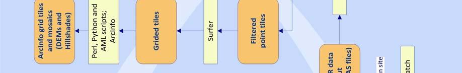
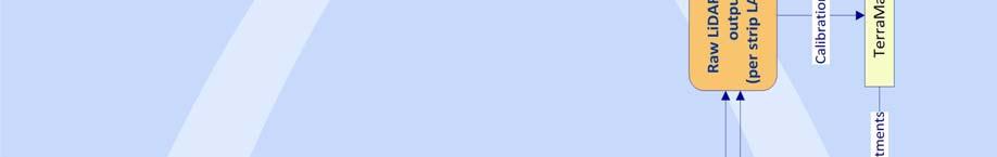
16 Fig 10 Laser data processing workflow 16

17 Figure 11. Laser processing QA/QC procedures 17

18 6. Classification TerraSolid s TerraScan software was used to classify the raw laser point into the following categories: ground, non-ground (default), aerial points and low points. Because of the large size of the lidar data the processing had to be done in tiles. Each survey segment was imported into TerraScan projects consisting of 1000m x 1000m tiles aligned with the 1000 units in UTM coordinates. The classification process was executed by a TerraScan macro that was run on each individual tile data and the neighboring points within a 40m buffer. The overlap in processing ensures that the filtering routine generate consistent results across the tile boundaries. The classification macros consist of a core of three algorithms: 1) Removal of Low Points. This routine was used to search for possible error points which are clearly below the ground surface. The elevation of each point (=center) is compared with every other point within a given neighborhood and if the center point is clearly lower then any other point it will be classified as a low point. This routine can also search for groups of low points where the whole group is lower than other points in the vicinity. Parameters used: Search for: Groups of Points Max Count (maximum size of a group of low points): 6 More than (minimum height difference): 0.3 m Within (xy search range): 5.0 m 2) Ground Classification. This routine classifies ground points by iteratively building a triangulated surface model. The algorithm starts by selecting some local low points assumed as sure hits on the ground, within a specified windows size. This makes the algorithm particularly sensitive to low outliers in the initial dataset, hence the requirement of removing as many erroneous low points as possible in the first step. Figure 12. Ground classification parameters The routine builds an initial model from selected low points. Triangles in this initial model are mostly below the ground with only the vertices touching ground. The 18

19 routine then starts molding the model upwards by iteratively adding new laser points to it. Each added point makes the model follow ground surface more closely. Iteration parameters determine how close a point must be to a triangle plane so that the point can be accepted to the model. Iteration angle is the maximum angle between point, its projection on triangle plane and closest triangle vertex. The smaller the Iteration angle, the less eager the routine is to follow changes in the point cloud. Iteration distance parameter makes sure that the iteration does not make big jumps upwards when triangles are large. This helps to keep low buildings out of the model. The routine can also help avoiding adding unnecessary point density into the ground model by reducing the eagerness to add new points to ground inside a triangle with all edges shorter than a specified length. Ground classification parameters used: Max Building Size (window size): 40.0 m Max Terrain Angle: 88.0 Iteration Angle: 6.0 Iteration Distance: 2.0 m Reduce iteration angle when edge length < : 5.0 m 3) Below Surface removal. This routine classifies points which are lower than other neighboring points and it is run after ground classification to locate points which are below the true ground surface. For each point in the source class, the algorithm finds up to 25 closest neighboring source points and fits a plane equation through them. If the initially selected point is above the plane or less than Z tolerance, it will not be classified. Then it computes the standard deviation of the elevation differences from the neighboring points to the fitted plane and if the central point is more than Limit times standard deviation below the plane, the algorithm it will classify it into the target class. Below Surface classification parameters used: Source Class: Ground Target Class: Low Point Limit: 8.00 * standard deviation Z tolerance: 0.10 m During the processing of these data, two types of artifacts became of special interest and required semi-manual intervention in the data in order to clean up: the presence of craters (due to low points) in the filtered dataset and high aerial points in the unfiltered dataset (typically caused by fog). Because of the high frequency rate at which the Gemini laser scanner is operating, multi-path points are quite common, especially in the urban environment These are points artificially situated well beyond the true ground surface (>20m), due to multiple bounces of the laser beam before returning to the airborne sensor. These low points can vary from just a few points grouped together to a few dozen, making a fully automated attempt to remove them more challenging. In addition to the inherent muti-path problem which is common with these type of sensors, we also discovered that the third stop point data collected by the Gemini sensor has a high percentage of points slightly below the true ground surface (~ m) that were causing artifacts in the final ground model. Because all third stop points for a given range file represent only a small percentage of 19

20 the total number of laser returns (~2% or less, usually bellow 1%), these points were not used for the ground classification. After the first filtering and gridding iteration the resulted shaded relief maps were used to guide the manual removal of the remaining low points. Figure 13 depicts an example of this artifact and the low points that generate it. Figure 13. Low points cluster example. Left panel top view shaded relief map displaying crater artifacts. Right panel profile through the point cloud showing a cluster of low points (pink) A second special concern was the presence of fairly large areas of high aerial points that were created by weather conditions such as fog. The areas affected by this kind of artifact are identified based on the unfiltered shaded relief map and field notes. The ground points are not affected by this because the ground classification algorithm is block-minimum biased and aerial points are not affecting the resulted ground surface. After the ground surface is determined, a simple height above ground threshold filter (75-80m) is used to identify and re-classify the high aerial points and the unfiltered dataset is re-output for griding. 20

21 Figure 14. High aerial points creating artifacts in the unfiltered dataset 21

22 7. DEM production The point data is output from TerraScan in 1000m x 1000m tiles, with 40m overlap. Two sets of files are generated, in XYZ ASCII format: filtered (ground class) and unfiltered (ground and default classes). In the unfiltered dataset the outlier classes are excluded from output (aerial and low points), as well as the third stop points (see 5.Classification). The overlap is needed in order to generate a consistent interpolation across tile edges and it will be trimmed in the final tile DEMs. A set of tiles in the comprehensive format is also outputted, to be used by the GEON online distribution and processing center. The various file formats and file naming conversions are described in the next section. The point tiles are grided using Golden Software s Surfer 8 Krigging at 0.5m cell size, using a 5m search radius for the unfiltered point data and 25m for the filtered. The griding parameters are: Gridding Algorithm: Kriging Variogram: Linear Nugget Variance: 0.15 m MicroVariance: 0.00 m SearchDataPerSector: 7 SearchMinData: 5 SearchMaxEmpty: 1 SearchRadius: 5m (unfiltered), 25m (filtered) The resulting tiled Surfer grid sets are transformed using in-house Perl and AML scripts into ArcInfo binary seamless tiles at 0.5m cell size. Due to the large area covered by the NoCal segments and the ArcInfo software limitations it is not possible to create one large mosaic for the entire area so the 0.5m tiles are mosaiced at 1m resolution into 10Km wide segments. The point tiles are the corresponding grids and mosaics are all positioned in the ITRF2000 reference frame and projected into UTM coordinates Zone 10N, all units in meters. The elevations are heights above the ellipsoid. Because ArcInfo doesn t support directly this particular projection, the grids are assigned the following projection information: UTM Zone 10N, WGS84 (original) datum. 7.1 Special note on the NoCal LiDAR data georeferencing Users who intend to integrate the NoCal LiDAR data with other geospatial data (especially data referenced to datums other than WGS84) should be aware that alignment issues may occur because the data is positioned in the ITRF2000 reference frame. There are several iterations of the WGS84 datum definition and the most recent ones are tied to ITRF (which is continually in motion because it accounts for plate tectonic movements) and thus by simply specifying WGS84 as datum is not enough to clearly identify which 22

23 version is used. In fact, ArcInfo s WGS84 datum definition implies WGS83_original which is equivalent with the NAD83(CORS96) datum and doesn t account for plate tectonic velocities. Currently, ITRF2000 is equivalent to WGS84(G1150). Therefore, it is important to use the transformation that is appropriate for the version of WGS84 used by these data in order to minimize alignment errors. For instance, ArcGIS provides 8 different transformations for aligning NAD83 data with WGS84 data. Failure to select the correct datum transformation can yield mismatches greater than 1.5 meters ArcGIS users should also note that ESRI does not yet offer a transformation for WGS84 tied to ITRF00 (G1150), however the ITRF96-based WGS84 (G873 - the edition of ITRF previous to ITRF00) is only a few centimeters different than ITRF00 so transformations based on ITRF96 should work reasonably well. For example, ArcInfo users should use the NAD_1983_To_WGS84_5 transformation method for projecting the LiDAR data (now assumed to be WGS84(G873) which is equivalent to ITRF96) into NAD83. For more information about the currently supported ArcInfo transformation visit this webpage: The online HTDP (Horizontal Time Dependent Positioning) toolkit provides many resources and interactive point data transformation between the various reference frames: The users should also be aware that the elevation values of all datasets are heights above the ellipsoid (WGS84) and not orthometric heights. The ellipsoid-heights are measured along the ellipsoid normal in contrast to the orthometric heights which follow the direction of the gravity. In many applications the term elevation most commonly refers to the orthometric height of a point. Ellipsoid heights from GPS surveys are converted to traditional orthometric values by applying a geoid height using the latest geoid model from the National Geodetic Survey (NGS). The Corps of Engineers Coordinate Conversion (CORPSCON, currently at v.6.0) tool can be used to transform the point data (XYZ ASCII tiles) ellipsoid heights into NAVD88 elevations using various GEOID models, including the latest iteration - GEOID03. The converted point data files can be then re-grided to ArcInfo raster format using your preferred interpolation technique. CORPSCON can be downloaded from this address: 8. File formats and naming conventions The following datasets are provided: 1. unfiltered point cloud, 1km x 1km tiles with 40m overlap, in XYZ (Easting, Northing, Elevation) ASCII format. File naming convention: uxxx000_yyyy000.xyz 23

24 2. filtered point cloud, 1km x 1km tiles with 40m overlap in XYZ (Easting, Northing, Elevation) ASCII format. File naming convention: fxxx000_yyyy000.xyz (XXX000, YYYY000) are the coordinates of the tile s lower left corner, ignoring the overlap. So for a tile with complete point coverage (not an edge tile), the real extent of the data is Easting: (XXX000 40) to (XXX ) and Northing: (YYYY000 40) to (YYYY ). 3. comprehensive point cloud, 1km x 1km ASCII tiles with no overlap. File naming convention: cxxx000_yyyy000.xyz This format includes the following fields: gpstimestamp, x, y, z, intensity, class, flight_line gpstimestamp = gps timestamp of the week (Sunday = day 0). For absolute time referencing, the week can be determined based on the survey date for each segment as described in Appendix A, Sheet A. X, Y, Z = Easting, Northing and Elevation intensity = laser intensity index. Intensity values were normalized using a 1000m normal range during laser point processing. Class = classification id number. The class number is one of the following: 1 Default (includes vegetation and above the ground artificial structures) 2 Ground 3 3rd stop 7 Low point 9 Aerial Points 14 Isolated Points flight line = flight ID number. These numbers reflect the order in which the original LAS flight strip files were loaded into TerraScan and don t necessary correspond with the flight strip numbers. 4. unfiltered binary ESRI GRID elevation tiles and shaded relief maps, 0.5m cells size and 1km x 1km extent with no overlap. File naming convetion: ugxxx_yyyy - DEM ugxxx_yyyyshd - corresponding shaded relief map 5. filtered binary ESRI GRID elevation tiles and shaded relief maps, 0.5m cells size and 1km x 1km extent with no overlap. File naming convetion: fgxxx_yyyy - DEM fgxxx_yyyyshd - corresponding shaded relief map 24

25 Due to ArcInfo naming limitations the raster dataset names include only the most significant digits from the tile s lower left coordinates. For example, the unfiltered point tile uxxx000_yyyy000.xyz becomes the ArcInfo raster ugxxx_yyyy. 6. unfiltered binary ESRI GRID mosaics and shaded relief maps, 1m cells size and 10Km wide with no overlap. File naming convetion: umxxx_x X X - mosaic DEM umxxx_x X X shd - corresponding shaded relief map 7. filtered binary ESRI GRID mosaics and shaded relief maps, 1m cells size and 10Km wide with no overlap. File naming convetion: fmxxx_x X X - mosaic DEM fmxxx_x X X shd - corresponding shaded relief map The naming convention for the mosaics uses the 3 most significant digits of the horizontal extent of the data and is different from the tiles naming convention. The mosaic umxxx_x X X will extend from Easting XXX000 to Easting X X X

26 Appendix A 1. NoCal survey flight days overview Flite # Date Airport DOY Flight time Laseron Square KM Area surveyed 1 3/22/2007 PRB South Creeping 2 3/23/2007 PRB North Creeping, Watsonville, Paicines Calaveras 3 3/25/2007 WVI South Calaveras 4 3/28/2007 CCR San Gregorio, Seal Cove 5 3/28/2007 CCR Seal Cove 6 3/29/2007 CCR Santa Cruz Mountains 7 3/30/2007 CCR Peninsular SAF, PUC San Andreas 8 3/31/2007 CCR Central Calaveras, PUC Hayward South 9 4/1/2007 CCR PUC Pipeline, Hayward 10 4/1/2007 CCR Berkeley 11 4/3/2007 CCR North Calaveras, PUC Calaveras 12 4/4/2007 CCR SAF Olema, Tomales Bay, Peninsular refly 13 4/5/2007 CCR Green Valley, North Calaveras 14 4/8/2007 UKI Bodega Bay 15 4/9/2007 UKI Bodega Bay, Gualala 16 4/10/2007 UKI Rodgers Creek, Maacama South 17 4/12/2007 UKI Maacama North, Furlong East Maacama 18 4/13/2007 UKI Shelter Cove Furlong EW 19 4/13/2007 UKI Furlong EW 20 4/15/2007 UKI Furlong EW 21 4/16/2007 UKI Little Salmon 22 4/16/2007 UKI Little Salmon Totals

27 2. Survey parameters DOY System PRF Scan Angle Scan Cutoff Scan Frequency Swath Width (average m) Southern Creeping Northern Creeping Paicines Calaveras Watsonville Southern Calaveras San Gregorio Seal Cove SantaCruz Mountains (N, S) Peninsula SAF PUC Southern Hayward Central Calaveras USGS Hayward PUC Pipeline Tomales-Olema Green Valley Northern Calaveras Bodega Gualala Southern Maacama Northern Macama Furlong Maacama Furlong E-W Shelter Cove Furlong E-W Little Salmon

28 3. List of OSU navigation solution versions used for NoCal processing Section DOY Trajectory Used (Date) Southern Creeping 81 08/02/07 Northern Creeping 82 09/10/07 Paicines Calaveras 82 12/28/07 Watsonville 82 12/28/07 Southern Calaveras 84 08/02/07 San Gregorio 87 02/04/08 Seal Cove 87 02/04/08 SantaCruz Mountains (Northern and Southern) 88 09/10/07 Peninsula SAF 89 10/24/07 PUC Southern Hayward 90 08/02/07 Central Calaveras 90 08/02/07 USGS Hayward 91 08/03/07 PUC Pipeline 91 08/03/07 Northern Calaveras 93 12/28/07 Tomales-Olema 94 01/08/07 Green Valley 95 09/10/07 Bodega 98 12/28/07 Gualala 99 09/10/07 Southern Macama /08/08 Northern Macama /08/08 Furlong Macama /08/08 Furlong E-W /10/07 Shelter Cove /10/07 Furlong E-W /08/08 Little Salmon /08/08 Note: the highlighted rows indicate the segments that were processed using the final batch of trajectories delivered by OSU. These are considered an improvement over the previously delivered trajectories but because of NCALM time and staffing limitation the decision was made to use the new solutions only for the data segments that were not already processed at that time (Dec. 2007) 28

29 4. DashMap processing parameters DOY DashMap Version First Second Third Last Scale IMU Roll IMU Pitch IMU Heading