Design and Implementation of Low power High Speed. Floating Point Adder and Multiplier

Transcription

1 Design and Implementation of Low power High Speed Floating Point Adder and Multiplier Thesis report submitted towards the partial fulfillment of requirements for the award of the degree of Master of Technology In VLSI Design & CAD Submitted by Ridhi Seth Roll No Under the Guidance of Ms.Harpreet Vohra Assistant Professor, ECED Department of Electronics and Communication Engineering THAPAR UNIVERSITY PATIALA , INDIA JUNE

2

3 i

4 ACKNOWLEDGEMENT I wish to express my special thanks and deepest regards to my Thesis Adviser, Ms. Harpreet Vohra, Assistant Professor, Thapar University, Patiala for providing me invaluable guidance, suggestions, and support, which has helped me to submit this thesis in time. Ms. Harpreet Vohra has been an advisor in the true sense both academically and morally throughout this project work. I take this opportunity to express my gratitude and sincere thanks to Dr. A.K. Chatterjee, Professor & Head, Ms. Alpana Agarwal, P.G Coordinator, Electronics & Communication Engineering Department and Ms. Manu Bansal for their valuable advice and suggestion and for providing me the opportunity to complete my seminar and thesis work simultaneously. I would also like to thank all the staff members of Electronics & Communication Engineering Department for providing me all the facilities required for the completion of this work. Appreciation is expressed to Prof. R.K. Sharma, Dean of Academic Affairs for providing me support to go ahead with my M.E. Thesis work. I wish to thank all my classmates for their time-to-time suggestions and cooperation. Finally it is the support, encouragement and good wishes of my parents and other family members without whom I would not have been able to complete my thesis. I thank and owe my deepest regards to all of them and all others who have helped me directly or indirectly. RIDHI SETH Roll no: ii

5 ABSTRACT A fast and energy-efficient floating point unit is always needed in electronics industry especially in DSP, image processing and as arithmetic unit in microprocessors. Many numerically intensive applications require rapid execution of arithmetic operations. Addition is the most frequent operation followed by multiplication. The demand for high performance, low Power floating point adder cores has been on the rise during the recent years. Since the hardware implementation of floating point addition involves the realization of a multitude of distinct data processing sub-units that endure a series of power consuming transitions during the course of their operations, the power consumption of floating point adders are, in general, quite significant in comparison to that of their integer counterparts. Multiplier is an important element which contributes substantially to the total power consumption of the system. Speed is a key parameter while designing a multiplier for a specific application. The objective is to design a 32 bit single precision floating point adder/subtractor and floating point multiplier operating on the IEEE 754 standard floating point representations. Second objective is to model the behavior of the Floating point adder and multiplier design using VHDL. The design of a low power and high speed adder and multiplier is thus the goal of my thesis work. The projected plan is to instantiate a good design and modify it for low power and high speed. The pipelining of these designs target high throughput computations. iii

6 ABBREVIATIONS CLB DSP FP FPGA FPU FSM HDL IEEE NRE RTL UCF VHDL VHSIC VLSI Combinational Logic Blocks Digital Signal Processing Floating Point Field Programmable Gate Arrays Floating Point Unit Finite State Machine Hardware Description Language Institute of Electrical and Electronics Engineers Non Recurring Engineering Register Transfer Level User Constraints File VHSIC Harware description Language Very High Speed Integrated Circuit Very Large Scale Integration iv

7 TABLE OF CONTENTS CERTIFICATE i ACKNOWLEDGEMENT.....ii ABSTRACT iii ABBREVIATIONS iv LIST OF FIGURES viii LIST OF TABLES ix CHAPTER 1 INTRODUCTION Need of floating point Operations Objectives Tools Used Organisation of this Thesis Literature Survey IEEE-754 Standard IEEE-754 Floating Point Data Formats Single Precision Floating Point Format IEEE 754 Standard data format Definitions IEEE Exceptions Rounding Modes...10 CHAPTER 2 FLOATING POINT ADDER Floating Point Addition Literature Review Methods of performing Floating Point Addition Triple Data Path Floating Point Adder Floating Point Adder Normalization.21 v

8 2.3 Proposed Design Pipelining Pipelined Floating Point Addition Module Pipelined Floating Point Subtraction Module...29 CHAPTER 3 FLOATING POINT MULTIPLIER Floating Point Multiplication Partial Products Generation and Reduction Floating Point Multiplication Algorithms Radix-2 Algorithm Booth s Algorithm Modified Booth Encoding Algorithm (Radix-4 Algorithm) or Booth-MacSorley recoding Partial Products Addition Carry look-ahead adder (CLA) Carry-Save Adder Final Adder Proposed Design Dual Path Floating Point Multiplier Pipelined Floating Point Multiplication Module...47 CHAPTER 4 FPGA IMPLEMENTATION Introduction to FPGA FPGA for Floating Point Computations FPGA Technology Trends FPGA Implementation Overview of FPGA Design Flow Procedure for Implementing the Design in FPGA Implementing the Design Assigning Pin Location Constraints Download Design to the Spartan-3E vi

9 Demo Board LCD and KEYBOARD Interfacing LCD Interfacing in FPGA Keyboard Interfacing in FPGA.62 CHAPTER 5 RESULTS AND CONCLUSION Simulation and Discussion Xilinx Results of Floating Point Adder FP adder simulation result RTL of FP adder Design summary of FP adder Modelsim Results of FP Adder Block Diagram Visualisation of Pipelining in FP adder Xilinx Results of Floating Point Multiplier Simulation results RTL Design Summary Modelsim Results of FP Multiplier Block diagram visualization of Floating Point Multiplier Conclusion.72 REFERENCES vii

10 LIST OF FIGURES Figure No. Title of Figure Page No. Figure 2.1 Block diagram of Floating Point Adder Figure 2.2 Control/data flow architecture of triple data path floating point adder[4]...18 Figure 2.3 Finite State machine representation of FADD[7]...21 Figure 2.4 LOD[9]...22 Figure 2.5 LOP[9]..22 Figure 2.6 Proposed Pipelined Triple Paths Floating Point Adder TDFADD..24 Figure 3.1 Block Diagram of nxn bit Booth multiplier[21]...34 Figure 3.2 Modified booth s encoding[22]...35 Figure 3.3 Encoding Mechanism...36 Figure 3.4 4:2 Compressor block diagram[26]...40 Figure 3.5 Carry save adder block is the same circuit as the full adder[28]..41 Figure 3.6 One CSA block is used for each bit[28] Figure 3.7 Adding m n-bit numbers with a chain of CSA[28] Figure 3.8 A Wallace tree for adding m n-bit numbers[24]...44 Figure 3.9 Dual Path FP Multiplier...46 Figure 4.1 FPGA Design Flow...53 Figure 4.2 Pin Diagram of LCD Interfacing...61 Figure 4.3 Pin Diagram of Keyboard Interfacing...62 viii

11 LIST OF TABLES Table No. Title of Table Page No. Table 2.1 Comparison of Synthesis Results Table 2.2 Setting of zero_check stage status signals...26 Table 2.3 Setting of the implied bit...27 Table 2.4 Preliminary checks for add_sub module...27 Table 2.5 add_sub operation and sign fixing 28 Table 2.6 Preliminary checks for add_sub module..29 Table 2.7 add_sub operation and sign fixing...30 Table 3.1 Recoding in Booth Algorithm Table 3.2 Recoding in Modified Booth Algorithm..36 ix

12

13 Chapter 1 INTRODUCTION 1.1 Need of Floating point Operations There are several ways to represent real numbers on computers. Floating-point representation, in particular the standard IEEE format, is by far the most common way of representing an approximation to real numbers in computers because it is efficiently handled in most large computer processors. Binary fixed point is usually used in special-purpose applications on embedded processors that can only do integer arithmetic, but decimal fixed point is common in commercial applications. Fixed point places a radix point somewhere in the middle of the digits, and is equivalent to using integers that represent portions of some unit. Fixed-point has a fixed window of representation, which limits it from representing very large or very small numbers. Also, fixed-point is prone to a loss of precision when two large numbers are divided. Floating-point solves a number of representation problems. Floating-point employs a sort of "sliding window" of precision appropriate to the scale of the number. This allows it to represent numbers from 1,000,000,000,000 to with ease. The advantage of floating-point representation over fixed-point (and integer) representation is that it can support a much wider range of values. Floating-point representation the most common solution basically represents reals in scientific notation. Scientific notation represents numbers as a base number and an exponent. For example, could be represented as Floating-point numbers are typically packed into a computer datum as the sign bit, the exponent field, and the significand (mantissa), from left to right. In computing, floating point describes a system for representing numbers that would be too large or too small to be represented as integers. Numbers are in general represented approximately to a fixed number of significant digits and scaled using an exponent. The base for the scaling is normally 2, 10 or 16. The typical number that can be represented exactly is of the form: significant digits base exponent The term floating point refers to the fact that the radix point (decimal point, or, more commonly in computers, binary point) can "float"; that is, it can be placed anywhere relative 1

14 to the significant digits of the number. This position is indicated separately in the internal representation, and floating-point representation can thus be thought of as a computer realization of scientific notation. 1.2 Objectives The objective is to design a 32 bit single precision floating point unit operating on the IEEE 754 standard floating point representations, supporting the three basic arithmetic operations: addition, subtraction and multiplication. Second objective is to model the behavior of the Floating point adder and multiplier design using VHDL. The programming objective of the floating point applications fall into the following categories: Accuracy: The application produces that results that are close to the correct results. Performance: The application produces the most efficient code possible. Reproducibility and portability: The application produces results that are consistent across different runs, different set of built options, different compilers, different platforms and different architecture. Latency: The application produces a single output with in less time. Throughput: The application produces more number of tasks that can be completed per unit time. Area: The application produces less number of flip flops and slices. 1.3 Tools Used The tools used ill the thesis are as follows: Simulation Software: ISE 9.2i (Integrated System Environment) has been used for synthesis and implementation. ModelSim 6.1e has been used for modelling and simulation. Hardware used: Xilinx Spartan 3E (Family), XC3S5000 (Device), FG320 (Package) FPGA device. 2

15 Tool used HDL (Top Level source Type), XST-VHDL/VERILOG (Synthesis Tool). ISE Simulator -VHDL/VERILOG (simulator), and VHDL (Preferred Language). 1.4 Organisation of this Thesis The rest of the thesis is organized as follows: Chapter 2 includes the basic architectures and functionality of floating point adders; describes the various modules of the block diagram of the proposed adder. Chapter 3 includes the basic architectures and functionality of floating point multipliers; describes the various modules of the block diagram of the proposed multiplier. Chapter 4 gives the basic description of the design methodology and design flow of FPGA, how the design is implemented on FPGA(Spartan 3E). After the proper simulation the design is synthesized and translated to structural architecture and then perform post translate simulations in order to ensure proper functioning of the device. The design is then mapped to the existing slices of FPGA and the post mapped module is simulated. The post map does not include the routing delays. After post mapped simulation the design is routed and a post route simulation model with appropriate routing delays is generated to be simulated on the HDL simulator. Chapter 5 gives the results and conclusion of thesis work, in terms of various results obtained during its implementation. 1.5 Literature Survey IEEE-754 Standard The IEEE floating-point standard, finalized in 1985, was an attempt to provide a practical floating-point number system that required floating-point calculations performed on different computers to yield the same result[1]. The IEEE (Institute of Electrical and Electronics Engineers) has standardized the computer representation for binary floating-point numbers in IEEE 754. This standard is followed by almost all modern machines. Notable exceptions 3

16 include IBM mainframes, which support IBM's own format (in addition to the IEEE 754 binary and decimal formats. Prior to the IEEE-754 standard, computers used many different forms of floating-point. These differed in the word-sizes, the format of the representations, and the rounding behavior of operations. These differing systems implemented different parts of the arithmetic in hardware and software, with varying accuracy. The IEEE-754 standard was created after word sizes of 32 bits (or 16 or 64) had been generally settled upon. Among the innovations are these: A precisely specified encoding of the bits, so that all compliant computers would interpret bit patterns the same way. This made it possible to transfer floating-point numbers from one computer to another. A precisely specified behavior of the arithmetic operations. This meant that a given program, with given data, would always produce the same result on any compliant computer. This helped reduce the almost mystical reputation that floating-point computation had for seemingly nondeterministic behavior. The ability of exceptional conditions (overflow, divide by zero, etc.) to propagate through a computation in a benign manner and be handled by the software in a controlled way IEEE-754 Floating Point Data Formats The standard provides for many closely-related formats, differing in only a few details[1]. Single precision: This is a binary format that occupies 32 bits (4 bytes) and its significand has a precision of 24 bits (about 7 decimal digits). Any integer with absolute value less than or equal to 2 24 can be exactly represented in the single precision format. Double precision: This is a binary format that occupies 64 bits (8 bytes) and its significand has a precision of 53 bits (about 16 decimal digits). Any integer with absolute value less than or equal to 2 53 can be exactly represented in the double precision format. Quadruple precision: This is another basic format that occupies 128-bits. 4

17 Sign Exponent Significand Bias Single precision 1[31] 8[30-23] 23[22-00] 127 Double precision 1[63] 11[62-52] 52[51-00] 1023 Quad 1[127] 15[ ] 112[111-00] Less common formats include: Extended precision format, 80-bit floating point value. Half also called float16, a 16-bit floating point value Single Precision Floating Point Format Single precision floating- point data are 32-bits wide and consist of three fields: a single sign bit (s), an eight- bit biased exponent (e) and a 23-bit significand(f). The number represented by the single-precision format is: value = (-1) s 2 e 1.f (normalized) when E > 0 else = (-1) s f (denormalized) where -1-2 n -23 n f = (b +b22 + bi + +b0 ) where bi =1 or 0 23 s = sign (0 is positive; 1 is negative) E =biased exponent; E =255, E =0. max min e =unbiased exponent; e = E 127(bias) Note that two representations of zero exist, one positive and one negative. There are five distinct numerical ranges that single-precision floating-point numbers are not able to represent: 1. Negative numbers less than -( ) (negative overflow) 2. Negative numbers greater than (negative underflow) 3. Zero 4. Positive numbers less than (positive underflow) 5. Positive numbers greater than ( ) (positive overflow) 5

18 Overflow means that values have grown too large for the representation, much in the same way that you can overflow integers. Underflow is a less serious problem because is just denotes a loss of precision, which is guaranteed to be closely approximated by zero IEEE 754 Standard data format Definitions The following terms are used extensively in describing the IEEE 754 floating point data formats This section is directly quoted from IEEE standard for Binary Floating Point Arithmetic[1]. Biased exponent: The sum of the exponent and a constant (bias) chosen to make the biased exponent s range nonnegative (Note the term exponent refers to a biased exponent.) Biased floating point : A bit string characterized by three components: a sing, a signed exponent and a significant its numerical value, if any, is the signed product of this significand and two raised to the power of its exponent. Denormalized: Denormalized numbers are those numbers whose magnitude is smaller than the smallest magnitude representable in the format. They have a zero exponent and a denormalized non-zero fraction. Denormalized fraction means that the hidden bit is zero. Fraction: The field of the significant that lies to the right of its implied binary point. Not A Number (NaN): IEEE 754 specifies a special value called Not a Number (NaN) to be returned as the result of certain invalid operations. They are used to signal invalid operations and as a way of passing status information through a series of calculations. NaNs arise in one of two ways. They can be generated upon an invalid operation or they may be supplied by the user as an input operand. NaN is further subdivided into two categories of NaNs, Signaling NaN (SNaN) and Quiet NaN (QNaN). They have the following format, where s is the sign bit: QNaN = S SNaN = S

19 The value is a quiet NaN if the first bit of the fraction is 1, and a signaling NaN if the First bit of the fraction is 0 (at least one bit must be non- zero). Signaling NaNs signal the invalid operation exception whenever they appear as operands. Quiet NaNs propagate through almost every arithmetic operation without signaling exceptions. Normalized: Most calculations are performed on normalized numbers. For single precision, they have a biased exponent range of 1 to 255, which results in a true exponent range of to The normalized number type implies a normalized significant (hidden bit is 1). The one to the left of the binary point is the so called hidden bit. This bit is not stored as part of the floating- point word; it is implied. For a number to be normalized, it must have this one to the left of the binary point. And for double precision true exponent range is to Significand: The component of a binary floating-point number that consists of an explicit or implicit or implicit leading bit to the left of its implied binary point and a fraction field to the right. True exponent: The component of a binary floating point number that normally signifies the integer power to which 2 is raised in determining the value of the represented number. Zero: The IEEE zero has all fields except the sign field equal to zero. The sign bit determines the sign of zero (i.e., the IEEE format defines a +0 and a -0). 7

20 Sign Exponent Fraction /Mantissa Value (positive zero) (negative zero) x0.(2-1 )= x x0.(2-23 ) (smallest value) x1.(2-2 )= x x 1.0 = infinity infinity Not a Number(NaN) Not a Number(NaN) IEEE Exceptions The IEEE standard defines five types of exceptions that should be signaled through a one bit status flag when encountered. These exceptions are invalid, overflow, underflow.and division by zero. Invalid Operation: The invalid operation exception is signaled if an operand is invalid for the operation to be performed. Some arithmetic operations are invalid, such as a division by zero or square root of a negative number. The result of an invalid operation shall be a NaN. The result of every invalid operation shall be a QNaN string with a QNaN or SNaN exception. The SNaN string can never be the result of any operation, only the SNaN exception can be signaled and this happens whenever one of the input operand is a SNaN string otherwise the QNaN exception will be signaled. The result, when the exception occurs 8

21 without a trap shall be a quiet NaN provided the destination has a floating-point format. The invalid operations are 1. Any operation on a signaling NaN 2. Addition or subtraction: Magnitude subtraction of infinities such as + ( ) Multiplication: ± 0 ± 3. Division:0 / 0 or / 4. Square root if the operand is less than Zero 5. Conversion of a binary floating- point number to an integer or decimal format when overflow infinity or NaN preclude a faithful representations in that format and this cannot otherwise be signaled. 6. Floating-point compare operations: when one or more of the operands are NaN. Inexact: This exception should be signaled whenever the result of an arithmetic operation is not exact due to the restricted exponent and/or precision range. Division by Zero: If the divisor is zero and the dividend is a finite nonzero number then the division by zero exception shall be signaled. Overflow: The overflow exception is signaled whenever the result exceeds the maximum value that can be represented due to the restricted exponent range. It is not signaled when one of the operands is infinity, because infinity arithmetic is always exact. Division by zero also doesn t trigger this exception. The result when no trap occurs shall be determined by the rounding mode and the sign of the intermediate result as follows: 1. Round to nearest carries all overflows to 1 with the sign of the intermediate result. 2. Round toward 0 carries all overflows to the format s largest finite number with the sign of the intermediate result. 3. Round toward- carries positive overflows to the formats largest positive finite number and carries negative overflows to Round toward + carries negative overflows to the formats most negative finite number, and carries positive overflows to

22 Underflow: An underflow exception is asserted when the rounded result is inexact and would be smaller in magnitude than the smallest normalized number in the specified format Rounding Modes Since the result precision is not infinite, sometimes rounding is necessary. To increase the precision of the result and to enable round-to-nearest-even rounding mode, three bits were added internally and temporally to the actual fraction: guard, round, and sticky bit. While guard and round bits are normal storage holders, the sticky bit is turned 1 when ever a 1 is shifted out of range. As an example we take a 5-bits binary number: If we left-shift the number four positions, the number will be , no rounding is possible and the result will no be accurate. Now, let s say we add the three extra bits. After left-shifting the number four positions, the number will be (remember, the last bit is 1 because a 1 was shifted out). If we round it back to 5-bits it will yield: , therefore giving a more accurate result. The standard specifies four rounding modes: Rounding to nearest (even), rounding toward zero, rounding to + and rounding to -. Rounding to nearest (even) is the standard s default mode; rounding toward zero is helpful in many DSP applications; and rounding to ± is used in interval arithmetic, which affords bounds to be specified on the accuracy of a number. Round to nearest even: This is the standard default rounding. The value is rounded up or down to the nearest infinitely precise result. If the value is exactly halfway between two infinitely precise results, then it should be rounded up to the nearest infinitely precise even. For example: Unrounded Rounded

23 Round-to-Zero: Basically in this mode the number will not be rounded. The excess bits will simply get truncated, e.g will be truncated to 3.4. Rounding to + / Round-Up: The number will be rounded up towards +, e.g. 3.2 will be rounded to 4, while -3.2 to -3. Rounding to - /Round-Down: The opposite of round-up, the number will be rounded up towards -, e.g. 3,2 will be rounded to 3, while -3,2 to

24 2.1 Floating Point Addition Chapter 2 FLOATING POINT ADDER Floating point addition is the most frequent floating point operation. FP adders are critically important components in modern microprocessors and Digital Signal Processors. The design of Floating Point Adders is considered more difficult than most other arithmetic units due to the relatively large number of sequentially dependent operations required for a single addition and the extra circuits to deal with special cases such as infinity arithmetic, zeros, NaNs. Standard Floating Point Addition requires following steps: Exponent difference Preshift for mantissa alignment Mantissa addition/subtraction Post shift for result normalization Rounding Addition of floating point numbers involves the prealignment, addition, normalization and rounding of significands as well as exponent evaluation. Significand prealignment is a prerequisite for addition. In floating point additions, the exponent of the larger number is chosen as the tentative exponent of the result. Exponent equalization of the smaller floating point number to that of the larger number demands the shifting of the significand of the smaller number through an appropriate number of bit positions. The absolute value of the difference between the exponents of the numbers decides the magnitude of alignment shift. Addition of significands is essentially a signed magnitude addition, the result of which operation is also represented in signed-magnitude form. Signed-magnitude addition of significands can lead to the generation of a carry out from the MSB position of the significand or the generation of leading zeros or even a zero result. Normalization shifts are essential to restore the result of the signed-magnitude significand addition into standard form. Rounding of normalized significands is the last step in the whole addition process. Rounding demands a conditional incrementing of the normalized significand. The operation of rounding, by itself can lead to 12

25 the generation of a cany out from the MSB position of the normalized significand. That means, the rounded significand need be subjected to a correction shifting in certain situations. Sign bits Exponents Significands Sign Exp. Comp. & Diff. Significand Selector Barrel Switch (Right Shift) Sign Magnitude Adder LZ Counter Normalization Shifter Exponent Corrector Rounding Logic Flag Logic Correction Shift Sign Flags Exp Significand Figure 2.1: Block diagram of Floating Point Adder Figure 2.1 illustrates the block diagram of a floating point adder. The exponent comparator and differencer block evaluates the relative magnitudes of the exponents as well as the difference between them. The significand selector block routes the significand of the larger number to the adder while routing the significand of the smaller number to the Barrel Switch. The Barrel Switch performs the requisite pre-alignment shift (right shift). The sign magnitude adder performs significand additiodsubtraction, the result of which is again represented in sign-magnitude form, The leading zero counter evaluates the number of 13

26 leading zeros and encodes it into a binary number. This block, essentially controls normalization shifts. The rounding logic evaluates rounding conditions and performs significand correction whenever rounding is necessary. The correction shift logic performs a right shift of the rounded significand if the process of rounding has resulted in the generation of a carry out from the MSB position of the significand. The exponent corrector block evaluates the value of the exponent of the result. The flag logic asserts various status flags subject to the validity of various exception conditions. Normalization Normalisation stage left shifts the significand to obtain leading 1 in the MSB, and adjusts the exponent by the normalisation distance. For true subtraction, the position of the leading 1 of the significand result is predicted from the input significands to within 1-bit using an LZA[19,20] which is calculated concurrently with the significand addition. The normalisation distance is passed to a normalization barrel shifter and subtracted from the exponent. Example: (binary) = x 2^11 (normalized binary) 2.2 Literature Review Methods of performing Floating Point Addition Implementations of FP adders are discussed in [2, 6, 12]. Algorithms and circuits which have been used to improve their design are described in [3, 5, 8, 10, 11, 15, 16, 17]. Traditional methods for performing FP addition can be found in Omondi [18] and Goldberg [4], who describe algorithms based on the sequence of significand operations: swap, shift, add, normalise and round. They also discuss how to construct faster FP adders. Some of these improvements are as follows: The serial computations such as additions can be reduced by placing extra adders (or parts thereof) in parallel to compute speculative results for exponent subtraction (Ea Eb and Eb - Ea) and rounding (Ma+Mb and Ma+Mb+1) then selecting the correct result (e.g. [9]). 14

27 By using a binary weighted alignment shifter, the calculation of the exponent differences (Ea Eb and Eb Ea) can be done in parallel with the significand alignment shift. The position of where the round bit is to be added when performing a true addition depends on whether the significand result overflows, so speculative computation of the two cases may be done[14]. Calculation of the normalisation distance can be done by a leading zero anticipator to provide the normalization shift to within one bit, in parallel with the significand addition [8]. Further improvements in speed can be made by splitting the algorithm into two parallel data paths based on the exponent difference [3, 15, 16], namely near ( Ea - Eb 1) and far ( Ea Eb > 1) computations, by noting that the alignment and normalisation phases are disjoint operations for large shifts. However there is a significant increase in hardware cost since the significand addition hardware cannot be shared as with the traditional three stage pipeline. Other FP adder designs have moved the rounding stage before the normalisation [5, 11, 12]. Quach and Flynn describe an FP adder [5] which uses a compound significand adder with two outputs plus a row of half adders and effectively has a duplicated carry chain. Hagihara et al. [6] report a 125 MHz FPU with a 3-cycle FP adder which adds three operands simultaneously, so two new operands can be accumulated per cycle, saving 25% of the accumulation execution time in a vector pipelined processor for use in supercomputers. Kowaleski et al. [12] describe an adder which contains separate add and multiply pipelines with a latency of 4-cycles at 43MHz. The significands are simultaneously added and rounded by employing a half adder which makes available a LSB for the case where a 1 is added for taking the two s complement of one input. Decode logic on two LSBs of both operands calculates if there will be a carry out of this section as a result of rounding, either by adding one or two. A circuit is used to determine if the MSB is 1 as a result of adding the significands in which case the round bit is added to the second LSB to compensate for the 15

28 subsequent normalization by 1-bit to the right. The significands are added by using a combination of carry look-ahead and carry select logic. Precomputed signals predict how far the rounding carry will propagate into the adder. The MSB computed before rounding is used to select the bitwise sums for the result. Nielsen et al. describes FP adder [15] with addition and rounding separated by normalisation. By using redundant arithmetic, the increment for the rounding is not costly. A variable latency architecture [16] has been proposed which results in a one, two, or three clock cycle data dependent addition. However, this implies that the host system can take advantage of up to three simultaneously emerging results, which represents a considerable scheduling difficulty. FP adders that have an accumulation mode or can bypass incomplete results are of interest in vector and deeply pipelined machines Triple Data Path Floating Point Adder The algorithms for addition and subtraction require more complex operations due to the need for operator alignment. Floating Point addition algorithm[4] Step 1 compare exponents compute exponent difference e1 - e2 evaluate special conditions 0 ± operand, ± ± operand, NaN ± operand select the tentative exponent of the result order significands on the basis of the relative magnitudes of exponents if e1 - e2 > p or special conditions, generate default result and go to step 2 if e1 - e2 <= 1 and subtraction go to step 3.1 if e1 - e2 > 1 or addition and neither e1 - e2 > p nor special conditions go to step 4.1 Step 2 present default result go to step 5 16

29 Step 3.1 perform 1 s complement addition of aligned significands perform speculative rounding count leading zeros of the different copies of results select result and pertinent leading zero count evaluate exception conditions, if any go to step 3.2 Step 3.2 normalize significand compute the exponent of the result go to step 5 Step 4.1 align the significand Step 4.2 perform signed-magnitude addition of aligned significands perform speculative rounding evaluate normalization requirements; 0 left or right shift select result and perform normalization select exponent evaluate exception conditions, if any go to step 5 Step 5 Select the appropriate copy of result from the relevant data path. 17

30 Exponents Data Selector Input floating point numbers Timing and Control Bypass Logic Significands Data Selector Exp. Incr/Decr 0/1 Bit Right Shifter Barrel Switch Exp. Selector Exp. Subtracter Flag Logic 1 s Comp. Adder & Rounding Logic Leading Zero Counter Result Selector Complementer 2 s Comp. Adder & Rounding Result Selector Flag Outputs Barrel Switch Result Integration Logic Right/Left Shifter Figure 2.2 : Control/data flow architecture of triple data path floating point adder[4] Figure 2.2 shows the control/data flow architecture of the triple data path floating point adder. In this scheme, the process of floating point addition is partitioned into three distinct categories and a separate data path is envisaged for each category. Among the three distinct data paths, two are computing data paths while the third is non computing (bypass) data path. The non computing or bypass data path becomes operational during those situations when the absolute value of the difference between the exponents ( e1-e2 ) exceeds the number of significand bits p (p represents the width of significand data field, including the hidden bit). The criterion for operational partitioning of the computing data paths is the possibility for the generation of variable number of leading zeros during the signed-magnitude addition of significands. A variable number of leading zeros can be generated only under two 18

31 circumstances - viz. subtraction of one significand from another when the difference between their exponents is zero or one. Significand pre-alignment shifts for this case are upper bounded by one. For other cases, signed-magnitude addition of significands can produce at the most one leading zero. Pre-alignment shifts, however, can be between 0 and p bit positions (p represents the width of significand data field, including the hidden bit) for such cases. The architecture offers power savings due to the simplification of data paths. Whenever the significand of a floating point number needs pre-alignment shifts, a pre-alignment shifter is mandatory for performing such an operation. In general, shifting of binary data through a variable number of bit positions demands complex hardware, the operational power demand and speed performance limitation of which units are expensive as far as hardware implementation of floating point adders is concerned. Since the architectural partitioning envisages a separate data path (left data path) for the handling of arithmetic operations that can probably lead to the generation of a variable number of leading zeros, this data path, however doesn t need a sophisticated Barrel Switch for significand pre-alignments. Since the pre-alignment shifts of input significands of this data path are upper bounded by one, the required alignment shifts can be performed by using a single level of MUXs. Though prealignment shifts are upper bounded by one for this data path (left data path), the normalization shift requirement can be anywhere between zero and p, by virtue of which it is mandatory to have a Barrel Switch for performing such shifts. The right data path (an arithmetic operation in this data path can produce at the most one leading zero), needs a prealignment Barrel Switch for significand alignments. The normalization shifter for this data path can be realized by using a single level of 3x1 MUXs. For the left data path, the 011 bit right shifter block handles the pre-alignment of input significands. This block also performs the complementation of the appropriate significand. The 1 s complement adder performs the signed magnitude addition of significands. Recomputation for rounding is performed concurrently with addition, so that by the time the rounding decisions are known, an appropriate copy of the result can be selected for normalization shift. The leading zero counting logic detects and encodes the number of leading zeros into appropriate binary words for each of the different copies of the results 19

32 generated by the 1 s complement adder/rounding logic. The FADD scheme employs a pseudo LZA approach for the estimation of leading zeros. Since the significand prealignment operation is rather fast for the left data path (due the absence of a Barrel Switch), the adder inputs of this data path get asserted at a relatively earlier time compared to that of the right data path. The earlier the arrival of significand inputs, the earlier the results of addition become available. Because of this reason, a full fledged leading zero anticipation logic (LZA) is not mandatory for this data path. Even with a simpler leading zero counting logic, this data path can complete the process of floating point addition within such time the right data path completes an addition. Effectively, this type of a scheme offers a speed performance that is comparable to that of schemes with full LZA while the complexity/area/power measures are appreciably less than that of schemes having full LZA. The result selection logic selects an appropriate copy of the result in accordance with the roundinglcomplementation conditions. This block also selects an appropriate copy of the leading zero count. The output (significand) of this block is shifted (left shift) by the Barrel Switch through an appropriate number of bit positions that is equal to the selected value of leading zero count. The exponent subtracter subtracts the relevant copy of leading zero count from the tentative exponent of the result. For the right data path, the input data selector selects significands for pre-alignment operation. The magnitude of pre-alignment shift is encoded by the control unit. The output of the pre-alignment Barrel Switch is routed to the significand adder through a complementer. The significand of the larger number is routed by the input data selector directly to the adder without any complementation. The complementer block performs a conditional inversion (bitwise) of its input data word. Complementation is performed only during the subtraction of one floating point number from the other. The 2's complement adder performs the signed magnitude addition of significands, the results of which operation are guaranteed to be positive all the time. Pre-computation for rounding is concurrently performed with addition. The result selector block selects an appropriate copy of the result according to the rounding/ normalization requirements. The normalization shifter for this data path is a simple left/right shifter. As explained earlier, the bypass data path becomes operational during those situations when the exponent difference is greater than the width of significands. This data path, essentially 20

33 selects and memorizes the larger floating point number. In pipelined architectures, the results of the bypass data path are not immediately presented to the output. Upon detection of a bypass condition, the larger floating point number is selected and latched by this data path. The latched data is presented to the output during an appropriate cycle of pipeline operation. The timing and control unit, flag logic and result integration logic are common to all the data paths. The timing and control unit evaluates the inputs for various conditions, selects an appropriate data path, routes the inputs to the selected data path, asserts flags and integrates the data from the relevant data paths to the final output. This unit generates the various gated clocks that control the data presentation to/from the various data paths. Figure 2.3 : Finite State machine representation of FADD[7] Among the three distinct data paths, two are computing data paths (the LZA and LZB data paths) while the third is a non computing (bypass) data path[7]. The LZA data path handles those cases of floating point addition (subtraction) which are likely to generate a significand with a variable number of leading zeros while the LZB data path handles the rest of the cases except that is handled by the bypass data path. The non computing or bypass data path becomes operational during those situations when the process of floating point addition is guaranteed to produce a result that is known apriori Floating Point Adder Normalization In order to increase the performance the floating point adder, several schemes are implemented to reduce the time required to normalize the final result. In the first stage of the adder an estimate is calculated for the number of left shifts needed to normalize the final result. This estimate is performed in parallel with the right shifter and adder, such that no additional time penalties are accrued during the first stage. During the second stage of the floating-point adder, the result of 21

34 the adder is left shifted by the value from the normalization estimate. The result of the left shifter is then used to generate several possible results, based on adder. This logic is used to determine if further shifting of the mantissa is required, or, if the final result is a denormal number. The direct way to perform the normalization is illustrated in Figure 2.4. Once the result of the addition has been computed, the Leading One Detector (LOD) determines the position of the leading one and then the result is left shifted. Alternatively, as shown in Figure 2.5, the shift amount can be determined in parallel with the significand s addition. The Leading One Predictor (LOP) anticipates the amount of the shift for normalization from the input operands. Input A Input B Input A Input B SIGNIFICAND ADDER/SUB. LOP SIGNIFICAND ADDER/SUB. LOD SHIFTER Shift Coding SHIFTER Shift Coding result result Figure 2.4: LOD[9] Figure 2.5: LOP[9] Leading One Predictor(LOP) Leading One Predictor anticipates the amount of shift for normalization from the input operands and this speeds up the operation. n bits of input produces log2 n bits of leading one Z count. 22

35 Comparison of Synthesis results for IEEE 754 Single Precision FP addition Using Xilinx 4052XL-1 FPGA[13] Parameters SIMPLE TDPFADD PIPE/ TDPFADD Maximum delay, D (ns) Average Power, P (mw)@2.38 MHz Area A, Total number of CLBs (#) Power Delay Product (ns. 10mW) Area Delay Product (10 #.ns) * * * * * * 10 4 Area-Delaly 2 Product (10#. ns 2 ) 7.13.* * * 10 6 Table 2.1: Comparison of Synthesis Results[13] 2.3 Proposed Design Pipelined Triple Paths Floating Point Adder (PTDFADD) A new architecture of speed and power optimized floating point adder is presented.. The functional partitioning of the adder into three distinct, inhibit controlled data paths allows activity reduction. During any given operation cycle, only one of the data paths is active during which time, the logic assertion status of the circuit nodes of the other data paths are held at their previous states. Critical path delay and latency are reduced by incorporating speculative rounding and leading one anticipation (prediction) logic. The latency of the floating point addition can be improved if the rounding is combined with addition/subtraction. LOP anticipates the amount of shift for normalization in parallel with addition [5]. 23

36 Exponents Input Floating Point Exponent Logic Control Logic Data Selector Pre-alignment (Barrel Shifter Right)/ Complementer Data Selector/Prealign (0/1 Bit Right Shifter) Critical Path Adder/Rounding Adder/Rounding Bypass Exponent Incr/Decr Result Selector Exponent Subtractor Result Selector Leading Zero Counter Normalization (1 bit Right/Left Shifter) Normalization (Barrel Shifter Left) Result Integration / Flag Logic Flag IEEE Figure 2.6: Proposed Pipelined Triple Paths Floating Point Adder TDFADD Pipelining Pipelining is one of the popular methods to realize high performance computing platform. It was first introduced by IBM in 1954 in Project Stretch. In a pipelined unit a new task is 24

37 started before the previous is complete. This is possible because most of the adders, high speed multiplies are combinational circuits. Once a gate output has been set it remains fixed for the remainder of the operation. Pipelining is a technique to provide further increase in bandwidth by allowing simultaneous execution of many tasks. A pipelined system divides the logic into stages separated by a set of latch registers. As soon as the output of a stage is latched, a new task can be started at the inputs to the stage. The latches keep the value of the old task which is input to the next stage. The bandwidth of the pipelined unit is the inverse of the latency per stage, not the latency of entire unit. As stage length is shortened bandwidth increases but as the number of stages increases, so does the number of latches necessary. While pipelining can result in sizeable increases in bandwidth, so can operating many units in parallel. Since a pipelined system processes many tasks at one time, the overall bandwidth / cost function should increase. In a pipelined system, the total latency is not as important as the latency per stage. It is important to reduce the total no of latches required since latches become a significant portion of the circuitry in a highly pipelined system. First in pipelined affects, the latches usually provide the necessary buffering. Second, the maximum fan-out of gates runs through wide range dependent on the manufactures. Implementing pipelining requires various phases of floating-point operations be separated and be pipelined into sequential stages. Pipelining is a technique where multiple instruction executions are overlapped. Design functionalities are validated through simulation and compilation. To achieve pipelining input processes must be subdivided into a sequence of subtasks, each of which can be executed by specialized hardware stage that operates concurrently with other stages in the pipeline. The adder design pipelines the steps, complementing, swapping, shifting, addition and normalization to achieve a summation every clock cycle.each pipeline stage performs operations independent of others. Input data to the added continuously streams in. Speed of operation of pipelined add has been found 3 times more than the unpipelined adder. Successful implementation of pipelining in floating point adder and multiplier using VHDL fulfills the needs for different high performance applications. 25

38 2.3.2 Pipelined Floating Point Addition Module Addition module has two 32-bit inputs and one 32 bit output. Selection input is used to enable or disable the module. Addition module is further divided into small modules: zero check, align, add_sub, and normalize modules. Unpacking Unpacking involves (i) Separating the sign, exponent and the significand for each operand and reinstating the hidden 1. (ii) Testing for special operands and exceptions ( e.g. recognizing NaN inputs and bypassing the adder). Zero check Module This module detects zero operands early in the operation and based on the detection result, it asserts two status signals. This eliminates the need of subsequent processes to check for the presence of zero operands. Table 2.2 summarizes the algorithm. Align Module Input a Input b Zero a1 Zero b Non-zero 1 0 Non-zero Non-zero Non-zero 1 1 Table 2.2: Setting of zero_check stage status signals In align module, operations are performed based on status signals from previous stage.zerooperands are checked in the align module as well. The module introduces implied bit into the operands that illustrated in Table 2.3. Selective Complementation module Complementation logic may be provided for only one of the two operands(typically the one that is not pre shifted, to shorten the critical path). If both operands have the same sign, the common sign can be ignored in the addition process and later attached to the result. Selective complementation and determination of the sign of the result are also affected by the +/- 26

39 control input of the floating point adder/subtractor which specifies the operation to be performed. Add_sub Module Zero a1 A sign YOR Zero b1 0 X(Don t implied bit for a Implied bit for b 0 0 Care) Table 2.3: Setting of the implied bit Add_sub module performs actual addition and subtraction of operands. Preliminary operands checking via the status signals are carried out first. Results are automatically obtained if either of the operands are zero (see Table 2.4). Normalization is needed if no calculations are done. The status signal norm is set to 0 for all cases. If both operands are not zero, the actual add_sub operation is done. A carry bit, introduced here, is tagged to the MSB of the result's mantissa. This gives an extra bit of precision and is useful for calculations involving a carry generation. The results are assigned to a stage3. Status signal is set to 1 to indicate the need for normalization by the next stage. Zero a2 AND Zero b2 Zero a1 XOR Zero b1 Zero a2 Result 0 0 X(Don t Care) Perform add sub b stage a stage2 1 X(Don t Care) X(Don t Care) 0 Table 2.4: Preliminary checks for add_sub module 27

40 Rounding Operation a sign a>b Result Sign fixing XOR B sign a + b 0 X(Don t Care) a + b Positive (-a)+(-b) 0 X(Don t Care) a + b Negative a+(-b) 1 Yes a - b Positive a+(-b) 1 No(b > a) b - a Negative (-a)+b 1 Yes a - b Negative (-a)+b 1 No(b > a) b - a Positive Table 2.5: add_sub operation and sign fixing The standard requires that all arithmetic operations are rounded so as to maintain high degree of accuracy and uniformity across different computing platforms as possible. Rounding operations wer originally viwed as a final separate step in most arithmetic circuit implementations. Rounding has been merged with addition in floating point adders by delaying normalization until after rounding[18]. Leading Zero Counter One of the main operations of floating point datapaths is normalization. During normalization the outcome of the floating point operation is brought to its normalized form according to the IEEE standard. Normalization involves the use of a leading zero counting(lzc), or detection unit and a normalization shifter. The problem of normalizing the result can be solved by counting the number of leading zeros of the result and then shifting the result to the left according to the outcome of the LZC unit[20]. The leading zero count is also required in order to correctly update the exponent part of the result. The predicted leading zero count is given to a shifter in order to normalize the true result. Normalize Module Input is normalized and packed into the IEEE754 floating-point representation. If the norm status signal is set, normalization is performed otherwise the implied and the carry bits at the mantissa's MSB is dropped. The result is then packed into the IEEE754 format and assigned to the output port. If norm is set, the module checks mantissa 1's MSB. This implies the carry bit is set and no normalization is needed. The carry bit is now the result's implied bit, which is dropped. The remaining bits are packed and assigned to the output port. 28

41 Packing Packing the result involves (i) Combining the sign, exponent, and the significand for the result and removing the hidden 1. (ii) Testing for special outcomes and exceptions (e.g. zero result, overflow or underflow) Pipelined Floating Point Subtraction Module Subtraction module has two 32-bit inputs and one 32-bit output. Selection input is used to enable/disable the entity depend on the operation. Subtraction module is divided further into four small modules zero check module, align module, add_sub module and normalize module. The subtraction algorithm differs only in the add_sub module where the subtraction operator change the sign of the result. The remaining three modules are similar to those in the addition module. Tab. 5 and Tab. 6 summarize the preliminary checks and sign fixing respectively for subtraction module. zero a2 AND zero b2 zero a2 XOR zero b2 zero a2 b sign Result Sign Fixing 0 0 X(Don t X(Don t Perform NA Care) Care) add sub b_stage2 b_sign= b_stage2 b_sign= X(Don t a_stage2 a_sign Care) 1 X(Don t Care) X(Don t Care) X(Don t Care) 0 NA Table 2.6: Preliminary checks for add_sub module 29

42 Barrel Shifter Operation a sign a>b Result Sign fixing XOR B sign (-a) - b 1 X(Don t Care) a + b Negative a - (-b) 1 X(Don t Care) a + b Positive (-a) - (-b) 0 Yes a - b Negative (-a) - (-b) 0 No(b > a) b - a Positive a b 0 Yes a - b Positive a b 0 No(b > a) b - a Negative Table 2.7: add_sub operation and sign fixing A barrel shifter is a digital circuit that can shift a data word by a specified number of bits in one clock cycle. It is used in the hardware implementation of floating-point arithmetic. For a floating-point add or subtract operation, the mantissa of the two numbers must be aligned, which requires shifting the smaller number to the right, increasing its exponent, until it matches the exponent of the larger number. This is done by subtracting the exponents, and using the barrel shifter to shift the smaller number to the right by the difference, in one cycle. If a simple shifter were used, shifting by n bit positions would require n clock cycles. Barrel shifters continue to be used in smaller devices because it has a speed advantage over software implemented ones. The designed circuit should shift a data word by any number of bits in a single operation. A N-bit shifter would require log2n number of levels to implement. For an 8 bit barrel shifter, it would require 3 logic levels. 30

43 Chapter 3 FLOATING POINT MULTIPLIER 3.1 Floating Point Multiplication With the constant growth of computer applications such as signal processing and computer graphics, fast arithmetic units especially multipliers are increasingly required. Advances in VLSI technology have given designers the freedom to integrate many complex components, which was not possible in the past. Multipliers are also used in many digital signal processing operations, such as correlations, convolution, filtering and frequency analysis, to perform multiplication. The most basic form of multiplication consists of forming the product of two positive binary numbers. This can be accomplished through the traditional technique of successive additions and shift in which each addition is conditional on one of the multiplier bits. Thus, the multiplication process may be viewed as consisting of the following two steps: 1. Evaluation of partial products. 2. Accumulation of the shifted party products. Therefore, to design a fast multiplier, either the number of the partial products or the time needed to accumulate the partial products should be reduced. It should be noted that binary multiplication is equivalent to a logical AND operation. Thus, evaluation of partial product consists of the logical ANDing of the multiplicand and the relevant multiplier bits, Each column of partial products must then be added and,if necessary any carry values passed to the next column. Steps of Multiplier s Design are (A) Partial products generation and reduction; (B) Partial products addition; and (C) The final adder. 3.2 Partial Products Generation and Reduction Floating Point Multiplication Algorithms There are a number of techniques used to perform multiplication. Various high-speed multipliers have been proposed and realized [21, 22, 23, 24, 25, 26]. One such technique is the Radix-n Multiplication system. A Radix-2 system computes the partial products by observing one bit of the multiplicand at a time. Higher radix multipliers can be designed to reduce the number of adders and hence the delay required to compute the 31

44 partial sums. The best known method is the Booth s algorithm which is a Radix-4 multiplication scheme. Booth s algorithm for a signed binary multiplication scheme, as modified by MacSorley, is widely used to design fast multipliers in computer hardware. Booth s algorithm performs the encoding serially. Modified booth s algorithm performs encoding in parallel way. These algorithms are discussed in detail Radix-2 Algorithm In order to start the algorithm, an imaginary 0 is appended to the right of the multiplier. Subsequently, the current bit xi and the previous bit xi-1 of the multiplier, x n-1 x n-2... x1x0 are examined in order to yield ith bit, yi of the recoded multiplier, y n-i y n-2... y1y0. At this point, the previous bit xi-l serves only as a reference bit. At its turn, xi-1 will be recoded to yield yi-1, with xi-2 acting as the reference bit. For i=o, its corresponding reference bit x-1 is defined to be zero. Table presents a summary on the recoding method used by the Booth's theorem. Xi Xi-1 Operations Comments Yi 0 0 Shift only String of zeros Shift only String of ones Subtract and Shift Beginning of string of ones Add and Shift End of string of ones 1 Table 3.1: Recoding in Booth Algorithm[21] Recoding multiplier- x n-1 x n-2...x1x0 in SD(sign digit) code Recoded multiplier- y n-1 y n-2... y1y0 x i x i-1 of multiplier examined to generate yi Previous bit - x i-1 - only reference bit i=0 - reference bit X-1=O 32

45 Simple recoding - yi = x i-1 X i Example in figure 4.2 shows the recoded version of the multiplier and figure 4.3 shows the multiplication using above technique. Multiplier (0) recoded as instead of 6 add/subtracts. Recoded Version of the multiplier Operand x (1) Recoded version y Example of Radix-2 Algorithm: A X x Y recorded multiplier Add A Shift Add A Shift Add A Shift The multiplication procedure uses recoding of the 2's compliment multiplier with the underlying fact that a k- long sequence of 1's is equivalent to a (k-l) long sequence of zero's. This replacement of string of 1's by 0's help reduce the partial products. Any arbitrary binary number can be recoded in this fashion, so that each group of 1 or more adjacent 1's gets substituted by minus 1 at its low end, a positive 1 to the left of its high end and intervening 33

46 0's. This recoding need not necessarily be performed in any predetermined order and can even be done in parallel for all bit positions. Drawback of Radix-2 Booth Algorithm The shortcoming of Booth algorithm is that it becomes inefficient when there are isolated l's. For example, (decimal 85) gets reduced to (decimal 85), requiring eight instead of four operations. This problem can be overcome by using high radix Booth algorithms Booth s Algorithm The Booth algorithm [21] is widely used in the implementations of hardware or software multipliers because its application makes it possible to reduce the number of partial products. It can be used for both sign-magnitude numbers as well as 2's complement numbers with no need for a correction term or a correction step. The advantage of Booth recoding is that it generates only half of the partial products compared to the multiplier implementation which does not use Booth recoding. However, the benefit achieved comes at the expense of increased hardware complexity. Y<n-1:0> Booth encoder and sign bits extension X<n-1:0> Partial product generator + adder s array n-bit adder P<n-1:0> Carry n-bit adder P<2n-1:n> Figure 3.1 : Block Diagram of nxn bit Booth multiplier[21] 34

47 3.2.4 Modified Booth Encoding Algorithm (Radix-4 Algorithm) or Booth-MacSorley recoding A modification of the Booth algorithm was proposed by MacSorley [22] in which a triplet of bits is scanned instead of two bits. This technique has the advantage of reducing the number of partial products by one half regardless of the inputs. The recoding is performed within two steps: encoding and selection. The purpose of the encoding is to scan the triplet of bits of the multiplier and define the operation to be performed on the multiplicand, as shown in Fig.below. This method is actually an application of a sign-digit representation in radix 4. The Booth- MacSorley algorithm, usually called the modified Booth algorithm or simply the Booth algorithm, can be generalised to any radix. For example, a 3 bit recoding would require the following set of digits to be multiplied by the multiplicand. Figure 3.2: Modified booth s encoding[22] The booth encoding algorithm is a bit-pair encoding algorithm that generates partial products which are multiples of the multiplicand. The booth algorithm shifts and/or complements the multiplicand (X operand) based on the bit patterns of the multiplier (Y operand). Essentially, three multiplier bits [Y (i+1), Y (i) and Y (i-1)] are encoded into nine bits that are used to select multiples of the multiplicand {-2X, -X, 0, +X, +2X}. The three multiplier bits consist of a new bit pair [Y (i+1), Y (i)] and the leftmost bit from the previously encoded bit pair [Y (i-1)] as shown in figure 3.3. Separately - x i-2 and x i-3 recoded into y i-2 and y i-3 - X i-4 serves as reference bit. 35

48 Groups of 3 bits each overlap - rightmost being x1 x0 (x-1), next x3 x2 (x1), and so on. Bits xi and x i-1 recoded into yi and y i-1 - X i-2 serves as reference bit. X7 X6 X5 X4 X3 X2 X1 X0 X(-1) y7y6 y5y4 y3y2 y1y0 Figure 3.3: Encoding Mechanism Isolated 0/1 handled efficiently. If xi-l is an isolated 1, yi-l = 1 - only a single operation needed. Similarly - xi-1 an isolated 0 in a string of 1's (1)... recoded as or single operation performed. The recoding of Modified Booth algorithm is shown in table Y i+1 Yi Yi-1 Encoded Digit Operand Multiplication * X * X * X * X * X * X * X * X Table 3.2 : Recoding in Modified Booth Algorithm [22] The general booth algorithm often uses sign extension which means that each partial product has its sign bit extended (repeated) to the leftmost MSB of the last partial product. The disadvantage of sign extension is that it increases the number of bits to add together. This require extra adders which decrease speed, increase power dissipation and increase area. A 36

49 modified version of the booth algorithm uses sign generation to eliminate sign extension. The sign extension is implements as follows: 1) Complement the sign or (m+ 1)th bit of each partial product. 2) Add 1 to the left of the sign bit of each partial product. 3) Add 1 to the sign bit of the first partial product. Example of Radix-4 Algorithm A X x Y recoded multiplier -A +2A -A operation Add -A bit Shift Add 2A bit Shift Add -A The advantage of sign extension is that it doesn't create an extra bit vector or partial product. Because we can insert the ones into the cells with half adder. Therefore, no extra adders are needed to implement the sign generation scheme. The modified booth encoding algorithm results in (n/2) [(n +1)/2, if n is odd] adder rows with each row consisting of m adders for an mxn-bit multiplication. This results in extremely regular and rectangular multiplication architecture. 37

50 Radix-4 Vs Radix-2 Algorithm (0) yields number of operations remains 4 the minimum (0) yields , requiring 4, instead of 3, operations. Compared to radix-2 Booth's algorithm - less patterns with more partial products; smaller increase in number of operations. Can design n-bit synchronous multiplier that generates exactly n/2 partial products, Even n - two's complement multipliers handled correctly; Odd n - extension of sign bit needed. Adding a 0 to left of multiplier needed if unsigned numbers are multiplied and n odd 2 0's if n- even. For an mxn-bit multiplication, the booth algorithm produces n/2 [(n+ 1)/2, if n is odd] partial products, each has a length of (m+ 1) bits. This can half the number of partial products. It reduces the number of adders by 50% which results in a higher speed, a lower power dissipation, and a smaller area than a conventional multiplication array [15]. 3.3 Partial Products Addition The final step in completing the multiplication procedure is to add the final terms in the final adder. This is normally called "Vector-merging" adder. The choice of the final adder depends on the structure of the accumulation array. Following is a list of fast adders which are normally used. 1. Carry look-ahead adder 2. Carry skip adder 3. Carry save adder 4. Carry- select adder The following sub sections discuss these adders briefly Carry look-ahead adder (CLA) The concept behind the CLA is to get rid of the rippling carry present in a conventional adder design. The rippling of carry produces unnecessary delay in the circuit. For a conventional adder the expressions for sum and carry signal can be written as follows. 38

51 S = A B C C = AB + BC + AC It is useful from an implementation perspective to define S and Co as functions of some intermediate signals G (generate), D (delete) and P (propagate). G= 1 means that a carry bit will be generated, P=l means that an incoming carry will be propagated to C0. These signals are computed as G = AB P = A B We can write S and C0 in terms of G and P. C0(G,P) = G + PC S(G,P) = P C Carry-Save Adder A Carry-Save Adder is just a set of one-bit fulladders, without any carry-chaining. Therefore, an n-bit CSA receives three n-bit operands, namely A(n-1)..A(0), B(n-1)..B(0), and CIN(n- 1)..CIN(0), and generates two n-bit result values, SUM(n-1)..SUM(0) and COUT(n- 1)..COUT(0). The most important application of a carry-save adder is to calculate the partial products in integer multiplication. This allows for architectures, where a tree of carry-save adders (a so called Wallace tree) is used to calculate the partial products very fast. One 'normal' adder is then used to add the last set of carry bits to the last partial products to give the final multiplication result. Usually, a very fast carry-lookahead or carry-select adder is used for this last stage, in order to obtain the optimal performance. For adding partial products, the popular technique which is used to enhance the adding speed uses carry-save adders. In this technique columns are added independently and in parallel with minimal carry propagation. Using this technique, we will reach two rows of sum outputs 39

52 and carry outputs which will be added in a conventional adder. There are different carry save adders: 3:2 counters, 4:2 compressors, etc. A 3:2 counter is a basic full adder which takes three bits and produces two bits, implying encoding three bits with two bits. A 4:2 compressor, on the other hand, takes five bits and produces three output bits, in which the third bit is used as the carry-in input in the other 4:2 compressor of the same stage. The block diagram of a 4:2 compressor is shown in figure 3.4. Figure 3.4: 4:2 Compressor block diagram[26] Several attempts to find repeatable patterns in Wallace trees have been made, leading to the notion of compressors such as 5:2 or 9:2. The notion of compressors has been a major departure from the traditional notion of Dadda counters, since they require the use of Carry- In and Carry-Out signals. However, the propagation of the signal is limited to 1 bit by rendering the Carry-In and the corresponding Carry-Out independent. The most popular compressor is actually the 4:2 compressor, introduced by Weinberger. 4:2 compressor basic characteristics are: The outputs represent the sum of the five inputs, so it is really a 5 bit adder. Both carries are of equal weighting, To avoid carry propagation, the value of Cout depends only on I1, I2, I3 and I4 and is independent of Cin. The Cout signal forms the input to the Cin of a 4:2 compressor of the next column. Carry-Save Addition Adding Multiple Numbers There are many cases where it is desired to add more than two numbers together. The straightforward way of adding together m numbers (all n bits wide) is to add the first two, then add that sum to the next, and so on. This requires a total of m 1 additions, for a total 40

53 gate delay of O(m lg n) (assuming lookahead carry adders). Instead, a tree of adders can be formed, taking only O(lgm lg n) gate delays. Using carry save addition, the delay can be reduced further still. The idea is to take 3 numbers that we want to add together, x + y + z, and convert it into 2 numbers c + s such that x + y + z = c + s, and do this in O(1) time. The reason why addition can not be performed in O(1) time is because the carry information must be propagated. In carry save addition, we refrain from directly passing on the carry information until the very last step. To add three numbers by hand, we typically align the three operands, and then proceed column by column in the same fashion that we perform addition with two numbers. The three digits in a row are added, and any overflow goes into the next column. Observe that when there is some non-zero carry, we are really adding four digits (the digits of x,y and z, plus the carry). Figure 3.5 : Carry save adder block is the same circuit as the full adder[28] Figure 3.5 shows a full adder and a carry save adder. A carry save adder simply is a full adder with the cin input renamed to z, the z output (the original answer output) renamed to s, and the cout output renamed to c. Figure 3.6: One CSA block is used for each bit. This circuit adds three n = 8 bit numbers together into two new numbers[28] 41

54 Figure 3.6 shows how n carry save adders are arranged to add three n bit numbers x,y and z into two numbers c and s. Note that the CSA block in bit position zero generates c1, not c0. Similar to the least significant column when adding numbers by hand (the blank ), c0 is equal to zero. Note that all of the CSA blocks are independent, thus the entire circuit takes only O(1) time. To get the final sum, we still need a LCA, which will cost us O(lg n) delay. The asymptotic gate delay to add three n-bit numbers is thus the same as adding only two n- bit numbers. The important point is that carry (c) and sum (s) can be computed independently, and furthermore, each ci (and si) can be computed independently from all of the other c s (and s s). This achieves our original goal of converting three numbers that we wish to add into two numbers that add up to the same sum, and in O(1) time. To add m different n-bit numbers together the simple approach is just to repeat this trick approximately m times over. There are m 2 CSA blocks (each block in the figure 3.6 actually represents many one-bit CSA blocks in parallel) that we have to go through, and then the final LCA. Note that every time we pass through a CSA block, our number increases in size by one bit. Therefore, the numbers that go to the LCA will be at most n + m 2 bits long. So the final LCA will have a gate delay of O(lg (n + m)). Therefore the total gate delay is O(m + lg (n + m)). 42

55 Figure 3.7: Adding m n-bit numbers with a chain of CSA s[28] Instead of arranging the CSA blocks in a chain, a tree formation can actually be used. This is slightly awkward because of the odd ratio of 3 to 2. Figure 3.8 shows how to build a tree of CSAs. This circuit is called a Wallace tree. The depth of the tree is log 3/2 m. Like before, the width of the numbers will increase as we get deeper in the tree. At the end of the tree, the numbers will be O(n+logm) bits wide, and therefore the LCA will have a O(lg (n + logm)) gate delay. The total gate delay of the Wallace tree is thus O(logm + lg (n + logm)). 43

56 Figure 3.8: A Wallace tree for adding m n-bit numbers[24] Carry Save Adder Implementation Now that we have seen that the carry save adder trees are most efficiently implemented by putting together the (3,2) blocks, we must still address the issue of how to implement the (3,2) block (carry save adder) efficiently. Functionally, the carry save adder is identical to the full adder. The full adder is usually implemented with a reduced delay from Cin to Cout because the carry chain is the critical delay path in adders. Unfortunately, there is no single carry chain in the carry save adder trees in multipliers. Thus, it does not pay to make the delay shorter for one input by sacrificing delay on other inputs for carry save adders. Instead, carry save adders are normally implemented by treating the 3 inputs equally and trying to minimize delay from each input to the outputs.[27] 3.4 Final Adder After reaching two final rows of carry outputs and sum outputs a conventional adder must be used to reach the final multiplication result. This adder must be high speed enough to yield a high speed multiplier. 44

57 Comparison of 3 types of FP Multipliers using 0.22 micron CMOS technology[27] AREA (cell) POWER (mw) Delay (ns) Single Data Path FPM Double Data Path FPM Pipelined Double Data Path FPM

58 3.5 Proposed Design Dual Path Floating Point Multiplier Exponents Input Floating Point Numbers Exponent Logic Control/Sign Logic Significand Multiplier(Partial Product Processing) Bypass Logic Critical Path CSA / Rounding Logic Sticky Logic Path 2 Exponent Incrementer Result Selector / Normalization Result Integration / Flag Logic Flag bits IEEE product Figure 3.9: Dual Path FP Multiplier 46

59 3.5.1 Pipelined Floating Point Multiplication Module Multiplication entity has three 32-bit inputs and two 32-bit outputs. Selection input is used to enable or disable the entity. Multiplication module is divided into check zero, check sign, add exponent, and normalize and concatenate all modules, which are executed concurrently. Status signal indicates special result cases such as overflow, underflow and result zero. In this project, pipelined floating point multiplication is divided into three stages. Stage 1 checks whether the operand is 0 and report the result accordingly. Stage 2 determines the product sign, add exponents and multiply fractions. Stage 3 normalizes and concatenate the product. Check Zero module Initially, two operands are checked to determine whether they contain a zero. If one of the operands is zero, the zero_flag is set to 1. The output results zero, which is passed through all the stages and outputted. If neither of them are zero, then the inputs with IEEE754 format is unpacked and assigned to the check sign, add exponent and multiply mantissa modules. The mantissa is packed with the hidden bit' 1 '. Add exponent module The module is activated if the zero flag is set. Else, zero is passed to the next stage and exp_flag is set to 0. Two extra bits are added to the exponent indicating overflow and underflow. The resulting sum has a double bias. So, the extra bias is subtracted from the exponent sum. After this, the exp_flag is set to 1. Multiply mantissa module In this stage zero_flag is checked first. If the zero_flag is set to 0, then no calculation and normalization is performed. The mantissa flag is set to 0. If both operands are not zero, the operation is done with multiplication operator. Mantissa flag is set to 1 to indicate that this operation is executed. It then produces 46 bits where the lower order 32 bits of the product are truncated. 47

60 Check sign module This module determines the product sign of two operands. The product is positive when the two operands have the same sign; otherwise it is negative. The sign bits are compared using an XOR circuit. The sign flag is set to 1. Rounding The standard requires that all arithmetic operations are rounded so as to maintain high degree of accuracy and uniformity across different computing platforms as possible. Rounding operations wer originally viwed as a final separate step in most arithmetic circuit implementations. Rounding has been merged with addition in floating point adders by delaying normalization until after rounding[18]. Leading Zero Counter One of the main operations of floating point datapaths is normalization. During normalization the outcome of the floating point operation is brought to its normalized form according to the IEEE standard. Normalization involves the use of a leading zero counting(lzc), or detection unit and a normalization shifter. The problem of normalizing the result can be solved by counting the number of leading zeros of the result and then shifting the result to the left according to the outcome of the LZC unit[20]. The leading zero count is also required in order to correctly update the exponent part of the result. The predicted leading zero count is given to a shifter in order to normalize the true result. Normalize and concatenate all module This module checks the overflow and underflow after adding the exponent. Underflow occurs if the 9th bit is 1. Overflow occurs if the 8 bits is 1. If exp_flag, sign_flag and mant_flag are set, then normalization is carried out. Otherwise, 32 zero bits are assigned to the output. During the normalization operation, the mantissa's MSB is 1. Hence, no normalization is needed. The hidden bit is dropped and the remaining bit is packed and assigned to the output port. Normalization module set the mantissa's MSB to 1. The current mantissa is shifted left until a 1 is encountered. For each shift the exponent is decreased by 1. Therefore, if the mantissa's MSB is 1, normalization is completed and first bit is the implied 48

61 bit and dropped. The remaining bits are packed and assigned to the output port. The final normalized product with the correct biased exponent is concatenated with product sign. 49

62 Chapter 4 FPGA IMPLEMENTATION 4.1 Introduction to FPGA A field programmable gate array (FPGA) is a semiconductor device that can be configured by the customer or the designer after manufacturing hence the name field- programmable. Field Programmable gate arrays (FPGAs) are truly revolutionary devices that blend the benefits of both hardware and software. FPGAs are programmed using a logic circuit diagram or a source code in Hardware Description Language (HDL) to specify how the chip will work. They can be used to implement any logical function that an Application Specific Integrated Circuit (ASIC) could perform but the ability to update the functionality after shipping offers advantages for many applications. FPGAs contain programmable logic components called logic blocks, and a hierarchy of reconfigurable interconnects that allow the blocks to be wired together somewhat like a one chip programmable breadboard. Logic blocks can be configured to perform complex combinational functions or merely simple logic gates like AND and XOR. In most FPGAs, the logic block also includes memory elements, which may be simple flip flops or more complete blocks of memory. FPGAs blend the benefits of both hardware and software. They implement circuits just like hardware performing huge power, area and performance benefits over softwares, yet can be reprogrammed cheaply and easily to implement a wide range of tasks. Just like computer hardware, FPGAs implement computations spatially, simultaneously computing millions of operations in resources distributed across a silicon chip. Such systems can be hundreds of times faster than microprocessor-based designs. However unlike in ASICs, these computations are programmed into a chip, not permanently frozen by the manufacturing process. This means that an FPGA based system can be programmed and reprogrammed many times. FPGAs are being incorporated as central processing elements in many applications such as consumer electronics, automotive, image/video processing military/aerospace, base stations, networking/communications, super computing and wireless applications. 50

63 4.2 FPGA for Floating Point Computations With gate counts approaching ten million gates, FPGA s are quickly becoming suitable for major floating point computations. However, to date, few comprehensive tools that allow for floating point unit trade offs have been developed. Most commercial and academic floating point libraries provide only a small number of floating point modules with fixed parameters of bit-width, area and speed[29]. Due to these limitations, user designs must be modified to accommodate the available units. The balance between FPGA floating point unit resources and performance is influenced by subtle context and design requirements. Generally, implementation requirements are characterized by throughput, latency and area. 1. FPGAs are often used in place of software to take advantage of inherent parallelism and specialization. For data intensive applications, data throughput is critical. 2. If floating point computation is in a dependent loop, computation latency could be an overall performance bottleneck. 4.3 FPGA Technology Trends General trend is bigger and faster. This is being achieved by increases in device density through even smaller fabrication process technology. New generations of FPGAs are geared towards implementing entire systems on a single device. Features such as RAM, dedicated arithmetic hardware, clock management and transceivers are available in addition to the main programmable logic. FPGAs are also available with the embedded processors (embedded in silicon or as cores within the programmable logic fabric). 4.4 FPGA Implementation The FPGA that is used for the implementation of the circuit is the Xilinx Spartan 3E (Family), XC3S5000 (Device), FG320 (Package) FPGA device. The working environment/tool for the design is the Xilinx ISE 9.2i is used for FPGA Design flow of VHDL code. 51

64 4.4.1 Overview of FPGA Design Flow As the FPGA architecture evolves and its complexity increases. Today, most FPGA vendors provide a fairly complete set of design tools that allows automatic synthesis and compilation from design specifications in hardware specification languages, such as Verilog or VHDL, all the way down to a bit stream to program FPGA chips. A typical FPGA design flow includes the steps and components shown in Fig. Inputs to the design flow typically include the HDL specification of the design, design constraints, and specification of target FPGA devices [30]. We further elaborate on these components of the design input in the following: Design constraints typically include the expected operating frequencies of different clocks, the delay bounds of the signal path delays from input pads to output pads (I/O delay), from the input pads to registers (setup time), and from registers to output pads (clock-to-output delay). In some cases, delays between some specific pairs of registers may be constrained. The second design input component is the choice of FPGA device. Each FPGA vendor typically provides a wide range of FPGA devices, with different performance, cost, and power tradeoffs. The selection of target device may be an iterative process. The designer may start with a small (low capacity) device with a nominal speed-grade. But, if synthesis effort fails to map the design into the target device, the designer has to upgrade to a high-capacity device. Similarly, if the synthesis result fails to meet the operating frequency, he has to upgrade to a device with higher speed-grade. In both the cases, the cost of the FPGA device will increase in some cases by 50% or even by 100%. This clearly underscores the need to have better synthesis tools since their quality directly impacts the performance and cost of FPGA designs [30, 31]. 52

65 Source Code FRONT END Verify Behavior functionality Logic Synthesis Translate Technology Mapping BACK END Place and Route Bitstream Generation Bitstream FPGA Figure 4.1: FPGA Design Flow 53

66 Design Entity The basic architecture of the system is designed in this step which is coded in a Hardware description Language like VERlLOG or VHDL. A design is described in VHDL using the concept of a design module. A design module is split into two parts, each of which is called a design unit in VHDL. The module declaration represents the external interface to the design module. The module internals represents the internal description of the design module-its behavior, its structure, or a mixture of both. Behavioral Simulation After the design phase, create a test bench waveform containing input stimulus to verify the functionality of the verilog code module using a simulation software i.e. Xilinx ISE 9.2i for different inputs to generate outputs and if it verifies then proceed further, otherwise modifications and necessary corrections will be done in the HDL code. This is called as the behavioral simulation. Design Synthesis After the correct simulations results, the design is then synthesized. During synthesis, the Xilinx ISE tool does the following operations: a) HDL Compilation: The tool compiles all the sub-modules in the main module if any and then checks the syntax of the code written for the design. b) Design Hierarchy Analysis: Analysis the hierarchy of the design. c) HDL Synthesis: The process which translates VHDL or Verilog code into a device netlist formate, i.e. a complete circuit with logical elements such as Multiplexer, Adder/subtractors, counters, registers, flip flops Latches, Comparators, XORs, tristate buffers, decoders, etc. for the design. If the design contains more than one sub designs, ex. to implement a processor, we need a CPU as one design element and RAM as another and so on, and then the synthesis process generates netlist for each design element. Synthesis process will check code syntax and analyze the hierarchy of the design which ensures that the design is optimized for the design architecture, the designer has selected. The resulting netlist is saved to an NGC (Native Generic Circuit) file (for Xilinx Synthesis Technology (XST)). 54

67 d) Advanced HDL Synthesis: Low Level synthesis: The blocks synthesized in the HDL synthesis and the Advanced HDL synthesis are further defined in terms of the low level blocks such as buffers, lookup tables. It also optimizes the logic entities in the design by eliminating the redundant logic, if any. The tool then generates a 'netlist' file (NGC file) and then optimizes it. The final netiist output file has an extension of.ngc. This NGC file contains both the design data and the constraints. The optimization goal can be pre-specified to be the faster speed of operation or the minimum area of implementation before running this process. The level optimization effort can also be specified. The higher the effort, the more optimized is the design but higher effort can also be specified. The higher the effort, the more optimized is the design but higher effort requires larger CPU time (i.e. the design time) because multiple optimization algorithms are tried to get the best result for the target architecture. Design Implementation The design implementation process consists of the following sub processes: 1. Translation: The Translate process combines all the input netlists and constraints to a logic design file. This information is saved an a NGD (Native Generic Database) file. This can be done using NGD Build program and.ngd file describes the logical design reduced to the Xilinx device primitive cells. Here, defining constraints is nothing but, assigning the ports in the design to the physical elements (ex. pins, switches, buttons etc) of the targeted device and specifying time requirements of the design. This information is stored in a file named UCF (User Constraints File). Tools used to create or modify the UCF are PACE, Constraint Editor Etc. 2. Mapping: The Map process is run after the Translate process is complete. Map process divides the whole circuit with logical elements into sub blocks such that they can be fit into the FPGA logic blocks. That means map process fits the logic defined by the NGD file into the targeted FPGA elements (Combinational Logic Blocks (CLB), Input Output Blocks (lob)) and generates an NCD (Native Circuit Description) file which physically represents the design mapped to the components of FPGA. MAP program is used for this purpose. 55

68 3. Place and Route: Place and Route (PAR) program is used for this process. The place and route process places the sub blocks from the map process into logic blocks according to the constraints and connects the logic blocks. Example if a sub block is placed in a logic block which is very near to IO pin, then it may save the time but it may affect some other constraint. So tradeoff between all the constraints is taken account by the place and route process.the PAR tool takes the mapped NCD file as input and produces a completely routed NCD file as output. Output NCD file consist the routing information. 4. Bitstream Generation: The collection of binary data used to program the reconfigurable logic device is most commonly referred to as a "bitstream," although this is somewhat misleading because the data are no more bit oriented than that of an instruction set processor and there is generally no "streaming." While in an instruction set processor the configuration data are in fact continuously streamed into the internal units, they are typically loaded into the reconfigurable logic device only once during an initial setup phase. 5. Functional Simulation: Post-Translate (functional) simulation can be performed prior to mapping of the design. This simulation process allows the user to verify that the design has been synthesized correctly and any differences due to the lower level of abstraction can be identified. 6. Static timing analysis: Three types of static timing analysis can be performed that are: (i) Post-fit Static timing analysis: The timing results of the Post-fit process can be analyzed. The Analyze Post-Fit Static timing process opens the timing Analyzer window, which interactively select timing paths in design for tracing. (ii) Post-Map Static Timing Analysis: Analyze the timing results of the Map process. Post- Map timing reports can be very useful in evaluating timing performance. Although route delays are not accounted for the logic delays can provide valuable information about the design. If logic delays account for a significant portion (>50%) of the total allowable delay of a path, the path may not be able to meet your timing requirements when routing delays are added. Routing delays typically account for 45% to 65% of the total path delays.by identifying problem paths, redesign the logic paths to use fewer levels of logic, tag the paths for specialized routing resources, move to a faster device, or allocate more time for the path. If logic-only-delays account for much less (35%) than the total allowable delay for a path or timing constraint, then the place-and-route software can use very low placement effort levels, 56

69 In these cases, reducing effort levels allow to decrease runtimes while still meeting performance requirements. (iii) Post Place and Route Static Timing Analysis: Analyze the timing results of the Post- Place and Route process. Post-PAR timing reports incorporate all delays to provide a comprehensive timing summary. If a placed and routed design has met all of timing constraints, then proceed by creating configuration data and downloading a device. On the other hand, identify problems and the timing reports, try fixing the problems by increasing the placer effort level, using re-entrant routing, or using multi-pass place and route. Redesign the logic paths to use fewer levels of logic, tag the paths for specialized routing resources, move to a faster device, or allocate more time for the paths. (iv) Timing Simulation: Perform Post-Place and Route simulation after the design has been and routed. After the design has been through all of the Xilinx implementation tools, a timing simulation netlist can be created. This simulation process allows to see how the design will behave in the circuit. Before performing this simulation it will benefit to create a test bench or test fixture to apply stimulus to the design. After this a.ncd file will be created that is used for the generation of power results of the design. 4.5 Procedure for Implementing the Design in FPGA The Spattan-3E Starter Kit board highlights the unique features of the Spartan-3E FPGA family and provides a convenient development board for embedded processing applications. The board highlights these features: Spartan-3E FPGA specific features Parallel NOR Flash configuration MultiBoot FPGA configuration from Parallel NOR Flash PROM SPI serial Flash configuration Embedded development MicroBlaze 32-bit embedded RISC processor PicoBlaze 8-bit embedded controller 57

70 DDR memory interfaces Implement the design and verify that it meets the timing constraints after check syntax and synthesis Implementing the Design 1. Select the source file in the Sources window. 2. Open the Design Summary by double-clicking the View Design Summary process in the Processes tab. 3. Double-click the Implement Design process to view the Translate and Map Place & Route in the Processes tab. 4. Notice that after Implementation is complete, the Implementation processes have a Green check mark next to them indicating that they completed successfully without Errors or Warnings, 5. Locate the Performance Summary table near the bottom of the Design Summary. 6. Click the All Constraints Met link in the Timing Constraints field to view the Timing Constraints report. Verify that the design meets the specified timing requirements. 7. Close the Design Summary Assigning Pin Location Constraints 1. Verify that source file is selected in the Sources window. 2. Double-click the Floorplan Area/IO/Logic - Post Synthesis process found in the User Constraints process group. The Xilinx Pinout and Area Constraints Editor (PACE) opens. 3. Select the Package View tab. 4. In the Design Object List window, enter a pin location for each pin in the Location column using the following information: CLK input port connect to FPGA pin C9 RDY_ OUT input port connect to FPGA pin L13 VAL_IN input port connect to FPGA pin L14 SF_CE0 input port connect to FPGA pin D 16 58

71 LCD _RS input port connect to FPGA pin L18 LCD _RW input port connect to FPGA pin L17 LCD _ E input port connect to FPGA pin M18 LCD _ 4 input port connect to FPGA pin R15 LCD_5 input port connect to FPGA pin R16 LCD _ 6 input port connect to FPGA pin P17 LCD _7 input port connect to FPGA pin M15 5. Select File to Save. You are prompted to select the bus delimiter type based on the Synthesis tool you are using. Select XST Default and click OK. 6. Close PACE. Notice that the Implement Design processes have an orange question mark next to them, indicating they are out-of-date with one or more of the design files. This is because the UCF File has been modified Download Design to the Spartan-3E Demo Board This is the last step in the design verification process. This section provides simple Instructions for downloading the counter design to the Spartan-3 Starter Kit demo board. 1. Connect the 5V DC power cable to the power input on the demo board (J4). 2. Connect the download cable between the PC and demo board (J7). 3. Select Implementation from the drop-down list in the Sources window. 4. Select lcd_fp_adder in the Sources window. 5. In the Process window, double-click the Configure Target Device process. 6. The Xilinx webtalk Dialog box may open during this process. Click Decline. 7. In the Welcome dialog box, select Configure devices using Boundary-Scan (JTAG). 8. Verify that automatically connect to a cable and identify Boundary-Scan chain is selected. 9. Click Finish. 59

72 10. If you get a message saying that there are two devices found, click OK to continue. The devices connected to the JTAG chain on the board will be detected and displayed in the impact window. 11. The Assign New Configuration File dialog box appears. To assign a configuration file to the XC3S500E device in the JTAG chain, select tile counter.bit file and click Open. 12. If you get a Warning message, click OK. 13. Select Bypass to skip any remaining devices. 14. Right-click on the XC3S500E device image, and select Program. The Programming Properties dialog box opens. 15. Click OK to program the device. When programming is complete, the Program Succeeded message is displayed. On the board, LCD Display the output of source file. 4.6 LCD and KEYBOARD Interfacing A programming file is generated by running the Generate Programming File process. This process can be run after the FPGA design has been completely routed. The Generate Programming File process runs BitGen, the Xilinx bitstream generation program, to produce a bitstream (.BIT) or (.ISC) file for Xilinx device configuration. The FPGA device is then configured with the.bit file using the JTAG boundary scan method. After the Spartan device is configured for the intended design, then its working is verified by applying different inputs LCD Interfacing in FPGA The figure 4.2 shows represent the implementation of LCD Interfacing of Double Precision Floating Point Square root. The representation has eleven ports: 1) CLK: It is the input clock. 2) RDY _OUT: It is the input wire of double precision floating point square root, it is ready to accept output. 3) VAL_IN: It is the input wire of double precision floating point square root, it is valid input value. 60

73 4) LCD_E: It is the output register, Read/Write Enable Pulse '0' for Disabled. '1' for Read/Write operation enabled. FPGA pin number is M18. CLK LCD_E LCD_RS LCD_RW RDY_OUT LCD_FP_adder LCD_4 LCD_5 LCD_6 LCD_7 Figure 4.2: Pin Diagram of LCD Interfacing 5) LCD_RS: It is the output register, Register Select '0' for Instruction register during write operations, Busy Flash during read operations. '1' for Data for read or writes operations, FPGA pin number is L18. 6) LCD_RW: It. is the output register, Read/Write Control 0 for WRITE, LCD accepts data. '1' for READ, LCD Presents data. FPGA pin number is L17. 7) LCD_4: It is the output register. Data bit is DB4 and FPGA pin number is R15. 8) LCD_5: It is the output register. Data bit is DB5 and FPGA pin number is R16. 9) LCD_6: It is the output register. Data bit is DB6 and FPGA pin number is P17. 10) LCD_7: It is the output register. Data bit is DB7 and FPGA pin number is M15. 11) SF_CEO: It is the output register, when the Strata Flash memory is disabled (SF_CEO = High), then the FPGA application has full read/write access to the LCD. 61

74 4.6.2 Keyboard Interfacing in FPGA The figure 4.3 shows represent the implementation of Keyboard Interfacing of CLK LCD_E PS2_CLK_IN LCD_RS LCD_RW PS2_DATA_IN RDY_OUT KEYBOARD_FP_adder LCD_5 LCD_6 RST_IN VAL_IN LCD_7 READY_OUT Figure 4.3: Pin Diagram of Keyboard Interfacing The representation has rest of the four ports: 1) PS2_CLK_IN: It is the input wire of PS/2 Clock line. FPGA pin number is G14. 2) PSE_DATA_IN: It is the input wire of PS/2 Data line, FPGA pin number is G13.. 3) RST_IN: It is the input wire of Asynchronous reset. 4) READY_OUT: It is the output register, this output high when module is output ready. 62

75 Chapter 5 RESULTS AND CONCLUSION 5.1 Simulation and Discussion The use of VHDL for modeling is especially appealing since it provides formal description of the system and allows the use of specific description styles to cover the different abstraction levels (architectural, register transfer and logic level) employed in the design. Design is verified through simulation, which is done in a bottom-up fashion. Small modules are simulated in separate testbenches before they are integrated and tested as a whole. 5.2 Xilinx Results of Floating Point Adder FP adder simulation result 63

76 5.2.2 RTL of FP adder 64

77 5.2.3 Design summary of FP adder 65

78 5.3 Modelsim Results of FP Adder Block Diagram Visualisation of Pipelining in FP adder 66

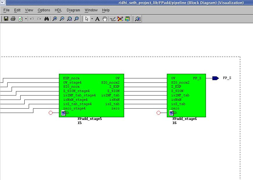
79 67

80 5.4 Xilinx Results of Floating Point Multiplier Simulation results 68

81 5.4.2 RTL 69

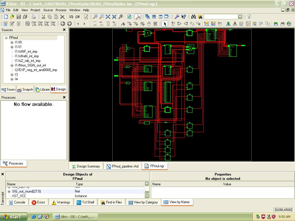
82 70

83 5.4.3 Design Summary of FP Multiplier 71

84 5.5 Modelsim Results of FP Multiplier Block diagram visualization of Floating Point Multiplier 5.6 Conclusion This work presents design, optimization and implementation of floating point arithmetic modules on FPGA to be used in DSP applications. These modules are floating point adder/subtractor and floating point multiplier. The architectural design of Pipelined Triple Data Path floating Point Adder incorporating techniques of throughput acceleration and power reduction is addressed. The latency of the floating point addition can be improved by combining rounding with addition/subtraction. Modified Booth s encoding is used to design a fast Dual Path Multiplier. Pipelining of the design targets high throughput computations. The simulation and synthesis results of modules are provided. 72