Top 15 Excel Tutorials

Transcription

1 Top 15 Excel Tutorials Follow us: TeachExcel.com

2 Contents How to Input, Edit, and Manage Formulas and Functions in Excel... 2 How to Quickly Find Data Anywhere in Excel... 8 How to use the Vlookup Function in Excel How to Use Multiple Functions and Formulas in a Single Cell in Excel How to Find and Fix Errors in Complex Formulas in Excel Calculate the Difference Between Two Times in Excel Quickly Convert Formulas into Their Output Values in Excel Enter a Constant Value in a Defined Name - Text, Numbers, Formulas, Etc Highlight Rows that Meet a Certain Condition in Excel How to import Text Files (CSV) into Excel How to View, Arrange, or Hide All Shapes, Charts, Pictures, Etc. in Excel Remove Gridlines in Excel 2007 and Later Install a Macro into an Excel Spreadsheet How to Make Macros Run A LOT Faster Run a Macro from Another Macro in Excel... 67

3 How to Input, Edit, and Manage Formulas and Functions in Excel Download the Excel file for this tutorial (link will be in the side bar or at the bottom of the page) In this tutorial I am going to introduce how to input, edit and manage excel formulas. To start entering a formula, you just select a cell and start typing with an equals sign first: Alternatively you can select the cell, then use the formula bar: When entering a Function into a formula make sure to use parenthesis/brackets to enclose the arguments:

4 To edit a formula you are unhappy with, simply select the cell and then the formula bar. You can then place the cursor at the part of the formula you wish to edit.

5 You can also edit any cell directly by double clicking on it. Formula/Function Helpful Features The Formula Auditing section of the Formula tab contains useful tools for managing your formula/functions and for checking/fixing errors. If you have linked cells in your formula you can select a formula and click the Trace Precedents/Dependents buttons help trace cell links.

6 The Show Formulas button does exactly that, displays the formulas in all the cells instead of their value. This allows you to see where all your formulas are. (Handy if youve got loads of different rows/columns of data. Showing the formulas can help you keep track of where they are and what they are doing. The Evaluate Formula button lets you step through the stages of a formula calculation. This allows you to see the order of operations of a formula and helps spot errors in calculations. The following window opens:

7 As you click Evaluate, Excel will step through the calculation part by part:

8 This is useful for spotting where your logic is wrong in a particular formula. This can be used in combination with the Error Checking/Tracing buttons to source any issues you may have with formula on a worksheet. The Error Checking evaluates all the cells in the worksheet and spots any cells with formula errors. The Error Trace button then helps find the root cause of a particular formula error. These features will help you maintain good working functions and spreadsheets in Excel.

9 How to Quickly Find Data Anywhere in Excel Download the Excel file for this tutorial (link will be in the side bar or at the bottom of the page) Finding specific records and/or cells is easy when using the Find tool in Excel. It is located within the Find & Select drop down on the Home tab. Just click on Find within that drop down (Ctrl + F works too) and the following window will open: To use Find you simply type the data you are looking for into the Find what text box. Above, I am looking for records which contain the text Tyler. I then

10 click Find Next. Excel then searches all the cells and selects the first cell it finds which contains Tyler. Alternatively I could have looked for Jackson and clicked Find All. This returns results based on the search: It shows me the number of times Jackson was found and what cells it was found in. If a search is unsuccessful, the following error message will appear:

11 As the pop-up advised I will now click the Options button to expand the options for the search. The Within drop down sets the scope of the search. Currently it is set to Sheet, so only searches within the current worksheet. As searching for was unsuccessful within Sheet I will change this to within Workbook. I click Find Next and the whole workbook will be searched for .

12 As you can see, this search was successful. Find took me to cell C1 on Sheet2 where it found a cell which contained . You may have noticed a number of other options within Find that I didnt use. Some of these are beyond the scope of this tutorial but I will give a brief description of these. The Search dropdown doesnt really matter unless your data set is quite large and you want to save time. It just defines how Find will search for your data. (Either column by column or row by row) As all my data is just simple text I dont need to change the Look in drop down. This is required when a workbook has lots of functions and formulas which I will cover how to use in a later tutorial. The match case and match entire cell contents checkboxes are pretty self-explanatory. They are used to refine a search. If you choose to match case, searching for TYLER for example would be different to searching for Tyler. If you choose to match entire cell contents then Excel will look for cells which entire cell value matches what you are looking for. So if you typed Tyl instead of Tyler with match entire cell contents enabled you wouldnt find anything in the dataset I provided. The Format options allow you to refine a search based on a cells formatting as well as its contents but this generally isnt used with Find. It is more commonly used with Find & Replace but this will be covered in a later tutorial as well.

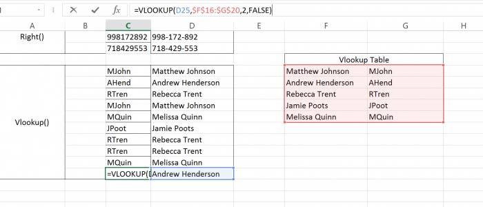
13 How to use the Vlookup Function in Excel (There is no Excel file to download for this tutorial. Here is another Vlookup Tutorial that might help.) Full explanation of the Vlookup function in Excel, what it is, how to use it, and when you should use it. The Vlookup function for Excel is a great function that allows you to search through a list of data within Excel. This allows you to do things like use the ID number of an item to locate other data for that item without having to manually go through a list of data. Though the function seems complex at first, it is quite easy to use once you become comfortable with the functions arguments. Here is the function listed with all of its arguments: =VLOOKUP(lookup_value, table_array, col_index_num, [range_lookup]) Below, each argument for this function is explained. lookup_value This is the actual thing/item/value/etc. that you want to use to locate the desired data contained within your Excel spreadsheet. This could be a unique ID number that attaches to a specific record; it could be a name; it could be a number that is contained within a range (explained in the range_lookup argument). Simply put, this is the value that is used to locate the data that you want to return. Once the Vlookup function finds this value, it will return data that is contained within the exact same row as where this value is found. The col_index_num argument below is where you tell the Vlookup function from which column you would like to return the data. Note that this value is searched for within the left-most column of data that is contained within the reference stated in the next argument, table_array. Also, you may use a cell reference for the lookup_value instead

14 of an actual value; this is a common technique that is used so that you can return different data without having to change the actual Vlookup function. table_array This argument tells the Vlookup function from which table of data you need to retrieve your values. For this argument, you will select a range of cells, for instance: A1:D10. In this example, the left most column is A and this is where the Vlookup function will try to find the lookup_value argument in order to return data from the corresponding row in which it is found. Make sure that you select a table_array that contains all of the data that you would like to return using the Vlookup function because you cannot return any data that is outside of this table array. col_index_num This is where you tell the Vlookup function which column contains the data that you would like to return. Following the example used in the table_array argument explanation above, if you want to return data from column C then you would put 3 for this argument. The columns are numbered starting with 1 for the left-most column referenced in the table_array argument. [range_lookup]) This is the only optional argument and its value can only be either TRUE or FALSE. This argument tells the Vlookup function if you want it to find an exact or approximate match. If you input FALSE, which is the most commonly used value for this argument, Excel will only return an exact match where the lookup_value exactly equals a value found in the left-most column of the table stated in the table_array argument. If this value is not found, it will return an error. If multiple values are found, the Vlookup function will return the first value that it finds. If you leave the value for this argument empty, since it is an optional argument, it will default to TRUE, which you can also manually enter

15 yourself. In this case, the Vlookup function will return an exact match if one is found, BUT, if an exact match is not found, it will return the next largest value that is less than the lookup_value. Also, in order for this to work, the first column of the table_array needs to be sorted in ascending order (the one that will be used to find the lookup_value). This TRUE value for the range_lookup argument is most often used when you want to return something that can be within a range, such as school grades, where an A or a B is not just a single number but, instead, can be achieved by having a grade that is within a range of numbers such as for a B and for an A. The Vlookup function is one of the most helpful functions that you will use within Excel. Though it may seem scary and confusing at first, just stick with it and you will be able to input this function in seconds and save yourself hours of sifting through data.

16 How to Use Multiple Functions and Formulas in a Single Cell in Excel Download the Excel file for this tutorial (link will be in the side bar or at the bottom of the page) Let s learn how to put multiple functions and formulas in a single cell in Excel in order to build more complex formulas that will, in the end, make your life easier. This is called nesting and it simply means putting functions inside of functions. All you have to do is start typing the function where you need it within another function. The basic concept that you need to understand is that you can put multiple functions within a single cell, inside of other functions (or next to other functions using concatenation - though concatenation is beyond the scope of this article). The best way to exhibit this, and my first experience with it, is with Text Manipulation in Excel. Let s say that you have the below example: We want to get the first two characters from each part number so we use the =LEFT() function in Excel to get this:

17 BUT, there is a problem with another list of values because some of them have spaces in front of them, so our LEFT() function on its own will not return what we want: Notice how for the first part number only "4" is returned when we want "4z". This is due to the space in front of the part number in cell B3. To solve this issue, we can nest functions; we can put another function inside the LEFT() function and this is as easy as typing the second function wherever we need it to work. Since we want to get rid of the extra spaces around some of the part numbers, we want to use the TRIM() function and we want to trim the part numbers before the LEFT() function pulls the two characters from the left of the text. As such, we put the TRIM() function around the cell reference for the part numbers like this:

18 You can see how the TRIM() function is placed completely inside of the LEFT() function. That is all there is to it. This is often used with the IF() function/statement in Excel to create more powerful logic statements. This is one of the most under-used, yet one of the most important, features of Excel and it allows you to make very powerful and complex analysis of data very quickly. You can nest many functions within a single cell, the number varies depending on your version, but a typical user will never reach that limit and, if you do, you are doing something wrong.

19 How to Find and Fix Errors in Complex Formulas in Excel (There is no Excel file to download for this tutorial.) Here, I'll show you a quick, simple, and effective way to fix formulas and functions in Excel. It can be hard to find out how to fix a formula or function in Excel that is broken or not returning the result that you expect. Thankfully, there is a really great tool that will help you troubleshoot the formula and pin-point the problem. It is called Evaluate Formula and it will save you hours! Below, I will give you a sample problem and show you, step-by-step, how to find and fix the error. Here, we have what should be a Vlookup formula that is not returning what we expect. Let's take a look at the formula now:

20 This is one formula that contains three functions, the IF function, the IFERROR function, and the VLOOKUP function. Looking at this, though it may seem a bit complex, everything appears to be input exactly how it should be. All functions look OK and the IF statement check at the front, that requires cell A6 to equal yes, looks good to me, but the formula is not working. Let's use the Evaluate Formula feature so that we dont waste any time troubleshooting this formula. Select the cell that contains the formula or function that is not working and then go to the Formulas Taband click the Evaluate Formula button, which is located in the Formula Auditing section of the menu.

21 The entire formula contents of the cell appear in the window. The Evaluate Formula feature will walk you through the execution of the entire formula and show you exactly what it sees. Notice how A6 contains an underline beneath it? This is what is evaluated first within this formula. Click the Evaluate button at the bottom of the window to see how Excel evaluates this, in this case, what it will return for the cell reference A6.

22 The value of cell A6 has been returned into this formula and we can see how Excel is now comparing that value to the value yes to see if they are equal. Hit Evaluate again. FALSE. We can see that the IF statement in the cell is preventing anything else from happening with this function because the condition in the IF statement has evaluated to FALSE. Hit the Evaluate button once more and you will see the final result, which is a blank. Now, hit the Restart button that appeared where the Evaluate button used to be and you can start over in order to more closely analyze everything. This, time, if you would like, you can hit the Step In button, which allows you, when possible, to enter a cell that is being referenced by the current formula. This feature is great for really complex formulas that are dependent upon many cells in Excel. If you do that in this case, everything still looks OK for cell A6. So, hit Step Out and let's get back to the main formula. Now, the next step has already been evaluated for us so we can see what cell A6 returns to the formula. Now, take a close look! CRAP!!!! There is a dirty stinking space after the yes in cell A6!!!! Let's correct that by closing the Evaluate Formula window and going to cell A6 to remove the space from the end of "yes" and try our vlookup formula again to see what happens.

23 It finally works! Now, we could have probably figured that out on our own after a while, but the Evaluate Formula feature showed very clearly, albeit, you must have been paying attention, that there was an extra space after the value coming from cell A6. Believe it or not, extra spaces, which are, by nature, difficult to find, cause many many many MANY hours of troubleshooting for people.

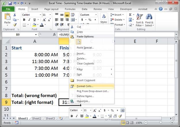
24 Calculate the Difference Between Two Times in Excel Download the Excel file for this tutorial (link will be in the side bar or at the bottom of the page) Here, you ll learn how to get the difference between two times in Excel. A common example of this is for when someone starts and finishes work. (Note that my version of Excel put the finish time in the 24 hour time format (military time) but that it is still just 5:45 PM.) Here we have a start and finish time and I want to see how much time has elapsed between them. All you need to do is to subtract the starting time from the finish time:

25 Excel will generally handle the rest. However, if the display of the new time does not look correct, it should be 7:45 in this case, then we need to make sure the formatting is right. Right-click the Time cell and select the Format Cells option. From there, a window will open up that looks like this:

26 Go to the Number tab and then select Custom from the Category section and make sure that you have selected h:mm from the area on the right. Then, hit OK and everything should work as you expect. Return the Hours, Minutes, or Seconds from the Time Difference in Excel You can also return just the Hours, Minutes, or Seconds from this result by using three simple functions, the HOUR(), MINUTE(), and SECOND() function. NOTE, these functions in the examples below will not return the total minutes or seconds between two times but will simply break that portion of the time out of the original result.

27 Here are the three functions: Here are the results of these functions: You can see how the total Time is 7 hours and 45 minutes and 0 seconds in cell C2.

28 These elements are simply broken out into their own cell using the HOUR, MINUTE, and SECOND functions above. Time is a very confusing element of Excel, but it can be quite powerful once you understand it. Make sure to visit TeachExcel.com for more Excel Time tutorials.

29 Quickly Convert Formulas into Their Output Values in Excel Download the Excel file for this tutorial (link will be in the side bar or at the bottom of the page) This tutorial teaches you how to convert a formula or function into its displayed output in Excel. This is very important and useful when you want to freeze a formula or function so that its output value cannot change. There is a very simply set of keyboard shortcuts that allows you to do this: First, select the desired functions/formulas then hit: Ctrl + C and then Alt + E + S + V and then hit Enter So, Ctrl + C > Alt + E + S + V > Enter Do this quickly and it will seamlessly convert all selected formulas/functions to their output value. All we are really doing is copying the cells then pasting-special their values in place of the functions/formulas. Here is a sample:

30 We have the RAND() function here and each time we update the spreadsheet (F9) these values will change: Now, let s make these values hard-coded. First, select the cells:

31 Hit Ctrl + C Then hit Alt + E + S + V and you will see this screen:

32 Hit OK and you are done! Now you can see that these values are actually numbers instead of the function RAND().

33 Enter a Constant Value in a Defined Name in Excel - Text, Numbers, Formulas, Etc. Download the Excel file for this tutorial (link will be in the side bar or at the bottom of the page) In Excel you can store values in Defined Names. Often people use a Defined Name to refer to a cell on a worksheet but that is just one small use for Defined Names. You can store text, numbers, formulas, and functions inside of a Defined Name all without referencing any cell in the worksheet or workbook. This allows you to hard-code values into a Name that you can then use within your formulas and functions throughout Excel. This is very easy to do - lets say that we want to store an interest rate in a Defined Name in Excel so we can use it in a calculation. First, go to the Formulas tab > Define Name

34 Once you click that, a window will open that allows you to enter all of the required data for your new Name: The name is what you will use to reference this Name and it should be simple and representative of the data that it will store. You can only use text, numbers, and underscores for a name. The scope allows you to limit a Names usability to a specific worksheet or the entire workbook but, usually, its best to keep this option as Workbook. Comment is a section where you can write something that will explain what this Name should be used for or what data it is storing or referencing. This comment will appear when you go to enter the name in the worksheet, as I will show you below. The Refers to: section is the most important as this is where the data, text, numbers, functions, formulas, or cell references will be entered. I will talk more about this section below as it can be a bit tricky. Here is what this box looks like when I fill-in the interest rate information that I want to use:

35 Once you hit OK, you have then created a name that can be used in any formula or function in Excel. Storing Different Types of Data in a Defined Name in Excel Now, let s talk about the Refers to: section. By default, this will have a cell reference of whichever cell is selected in the worksheet, like this: And that is how you should reference a cell, using Absolute Cell References (note the dollar signs), for a Defined Name.

36 Now, if you want to input text in the Defined Name, you need to surround it with quotation marks in the Refers to section like this: If you store numbers you do not need quotation marks, as shown in one of the examples above where I input an interest rate, which is just a decimal number. If you want to store a formula or function, you input it in the Refers to section just like you would in a cell in Excel: That is all there is to storing constant values and hard-coded values, numbers, text, etc. in a Defined name in Excel. Here is an example of using the interest_rate name in a function:

37 Notice in the FV function the first argument is interest_rate which is what we named the interest rate when we created that Defined Name. Also note that when you go to enter a Defined Name, it will appear in the drop-down menu that shows in Excel along with the comment that you entered when you created the Name:

38 The comment text only appears when you select the name from the drop down so, if you have many potential choices, the comments for each one dont appear until individually highlighted. As you can see, Defined Names are quite versatile and co do a lot more than just reference a boring old cell in Excel. This feature is very useful when creating large and complex spreadsheets. Note: If you click the Name Manager button on the formulas tab, you will be able to see all of the names in that are in the spreadsheet and you can then edit, delete, or add them from there.

39 Highlight Rows that Meet a Certain Condition in Excel Download the Excel file for this tutorial (link will be in the side bar or at the bottom of the page) In this tutorial I am going to cover how to highlight rows that meet a certain condition. To do this I use the Conditional Formatting tool. I will demonstrate some features of this advanced and powerful Excel tool. The Conditional Formatting dropdown is accessed from the Home tab: Conditional formatting involves applying a rule to the value of a cell. If this rule evaluates true then a certain format is applied to highlight that cell. If it is false then no formatting is applied. Note that cells which do not meet the rule still keep their original formatting. For the first example I am going to add a conditional formatting rule on the Order Total column. I am going to highlight orders which are over 5,000 in value. To do this, first I must select the Order Total column. I then navigate to the Highlight Cells Rules sub-menu of the conditional formatting menu.

40 I then select the Greater than option. The first box is the value I want my cells to be greater than. (5000 in this case) The second box is then the formatting that is to be applied to the cells with values greater than There are a number of default options here as well as a custom formats option, should you want to be specific. For this tutorial I went with a Green Fill with Dark Green Text.

41 Here is the result: As you can see a number of cells are now highlighted as they are over the Alternatively I could have done Order Totals less than 5000 or between 1000 and 5000, or whatever I wanted. There are a number of basic rules here that you can apply to highlight cell values you are most interested in. You can even do custom rules, but this is more on the advanced side of the conditional formatting tool and will be covered in a later tutorial. Conditional formatting doesn t just work on numerical values. You can highlight a cells value if it contains a certain text value. Although filtering may be a more useful tool for this I will demonstrate the functionality. For example I could highlight cells in the Country column where the order is from the United States.

42 Follow the same steps as before but, this time, select Equal to from the Highlight Cells Rules menu. It s the same as before, just enter the required value but this time Excel is checking whether the values of the County column are equal to United States.

43 Another useful conditional formatting rule is to highlight the top or bottom 10, 20, 50 etc. These rules are located in the Top/Bottom Rules sub-menu of the Conditional Formatting dropdown. As an example I am going to highlight the bottom 10 orders by Order Completion. As before I highlight the Order Completion column and then select Bottom 10 Items from the menus. A similar menu opens up prompting for the number of top/bottom items. As the default options are what I m looking for I just click ok.

44 You can also use filtering in combination with your conditional formatting so you can easily see just the conditionally formatted rows. To do this just right-click on a cell with the conditional formatting you want to filter and select Filter by Select Cells Color.

45 As I just highlighted the bottom 10 Order Completion cells I am going to apply a filter to see just those bottom 10 rows. As you can see only 10 rows are displayed. Should you want to remove a conditional formatting rule, you just select the cells you want to remove the conditional formatting from and then navigate to the Clear Rules sub-menu of the Conditional Formatting dropdown.

46 You can choose to remove the conditional formatting from the selected cells or the entire sheet should you require. For example, I am going to remove the conditional formatting on the Country column. Alternatively you could add/remove rules from the Manage Rules pop-up window. Just select it from the Conditional Formatting dropdown and then change the Show formatting rules for: box to worksheet. You then can see all the rules applied to the current worksheet. As you can see below the yellow formatting applied to the Country column is gone.

47 How to import Text Files (CSV) into Excel Download the Excel files for this tutorial (link will be in the side bar or at the bottom of the page) Text files in CSV format are one of the easiest ways to store and transfer data as it is one of the most compatible files to use. Even a basic text editor such as Notepad can understand them, although this is not recommended when you have 1,000s or even 10,000s of lines of text stored as it gets a bit confusing to read/navigate, and this is why you want to use Excel. CSV stands for Comma Separated Values and is a text file with a structure much like a table. Each column of the table is separated by a comma and each row is separated by a new line. In the last tutorial I had a list of forenames, surnames and ages. I now have this information in a CSV: Even looking at this CSV in Notepad you can see a table. It is this feature of CSVs that allows Excel to easily import them. To import a CSV you first select the DATA tab then left click From Text in the first panel. (Highlighted below)

48 The following window should appear: You just navigate to the CSV file you wish to import, select it and then click the Import button. A 3-step wizard will then open to help you import your text file correctly:

49 Step 1 has a number of options but most of these you will never change. The only thing to note here is if your data has column headings you will have to check the My data has headers checkbox. My CSV has column headings so I have this selected. You then click next.

50 Step 2 then appears as above. All you need to select here is Comma as your delimiter then click next. All the other options here are for files which are separated in various forms other than commas and you select those options if you need to. The Data preview window shows you what your data will look like with the selected delimiter so, if it doesn t look right, select another one until it does and then hit the Next button.

51 The third and final step allows you to select the data format of each of your columns. General format is selected for each column by default and will do most of the work here for you by converting numbers and dates where it deems appropriate. All remaining values are then just changed to text. You shouldn t need to change this very often unless you are importing data which Excel doesn t understand. This could be odd date formats or importing numbers that are too large for Excel which are better stored as text (e.g. long Order Numbers which have more than 15 digits). After you click finish you must select where you want the new data to be placed in excel.

52 Table is the only option I have here as it is such a small CSV. Larger files will have more options for PivotTables and PivotCharts but using these will be covered later. You can choose a new or existing worksheet by selecting the option then typing in the cell reference or alternatively you can click the box with an arrow to select the cell with the mouse. The data will then fill in to the right and downwards from your selection. I could have also clicked Finish on the first step and got the exact same result. Excel would have been able to automatically detect the structure and format of my simple CSV. You don t need to use the full wizard unless something isn t importing correctly.

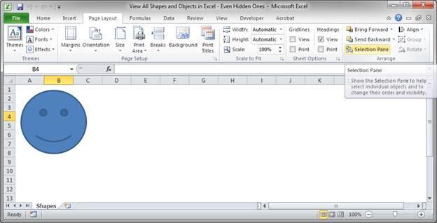
53 How to View, Arrange, or Hide All Shapes, Charts, Pictures, Etc. in Excel Download the Excel file for this tutorial (link will be in the side bar or at the bottom of the page) In Excel, you can add shapes, images, objects, photos, and all sorts of items to the spreadsheet. The problem is that sometimes these items can be hidden or can overlap each other such that you can t find them. But, there is a really great tool that allows you to view all of the objects that you have in your worksheet, it s called the Selection Pane. Here is a sample worksheet with some objects in it:

54 At this point, we can only see a smiley face, but, let s see if there is anything else in the worksheet. To get to the Selection Pane, select any object in the worksheet, click the Format tab that will then appear, then select the Selection Pane button: Once you click Selection Pane, you will see this:

55 Now, we can see that there are actually three shapes on the sheet. One is a smiley face, one a heart, and one is an oval these are the default names for these objects but they could have been renamed to anything. The first thing to notice is that there is no eye image next to the shape titled Oval 1 and this means that it is hidden. Simply click the white button where the eye should be to see it in the sheet:

56 You can also click the button Show All at the bottom of the Selection Pane window to quickly make all shapes and objects visible or Hide All to hide all of them. However, as you may have seen, there are three items on the worksheet but we can only see two of them. This happens when an object is on top of another one. To see if that is the case here, simply select the items in the Selection Pane and see where the outline for it appears on the worksheet. Tip: if you select a single item in the Selection Pane and then hit Ctrl + A, it will select all items at once so you can see them.

57 Here, it looks like there is something inside of the smiley face. To see if that is true, you can do one of two things: Click the smiley face with the mouse and drag it away:

58 Or, select the smiley face shape from the Selection Pane and then hit the down arrow at the bottom of the Selection Pane until an object appears on top of the smiley face:

59 Both ways let you see the object that is under the smiley face. I recommend using the second method since objects are often strategically placed within a worksheet and you don t wat to mess-up the placement of them. However, hitting Ctrl + Z will undo any changes in case you mess-up anything. If there are no visible shapes or objects in the worksheet but you know that some are there and you want to see them, you can still access the Selection Pane, just go to the Page Layout tab and click the Selection Pane button, which is located in the Arrange group of icons.

60

61 Remove Gridlines in Excel 2007 and Later (There is no Excel file to download for this tutorial.) In Excel 2007 and later you can quickly remove the gridlines that appear within the Excel worksheet. This allows you to view the worksheet without any lines in it. You won't see the outline of any cells and this may not seem like a good idea. However, this allows you to make really clean looking spreadsheets in Excel and allows you to put focus on certain elements within the spreadsheet. This is especially helpful when creating forms in Excel; when doing this you don't need or want extra gridlines within the spreadsheet. Remove or Add Gridlines in Excel 2007: View tab > Show/Hide box > Un-check the Gridlines check box Sales Report with Gridlines:

62 Sales Report without Gridlines:

63 Install a Macro into an Excel Spreadsheet (There is no Excel file to download for this tutorial.) This tip will show you how to copy an Excel Macro into your workbook or spreadsheet. You will learn the different locations that you might install the macro as well as what you need to make sure is included in the macro for it to work. First - Every macro must start and end like the example below: Sub The_Name_of_The_Macro() End Sub The code for the macro goes here. Every macro in Excel must start with "Sub" and end with "End Sub." The name of the macro must have an open and closed parenthesis right after it. You can name the macro anything that you want but you should make it describe the function of the macro. All of the actual code for the macro comes after the name of the macro and before "End Sub." Second - There are a number of different places where you can install a macro in Excel and you need to know this before you install the macro. You can install a macro into a Module, Worksheet, or Workbook - See Image Below.

64 How to install the Macro into Excel - Steps 1. Copy the code for the macro. Make sure to include the everything between the "Sub" and "End Sub." 2. Open the desired Excel workbook. 3. Hit "Alt + F11" on the keyboard (this shortcut works for all versions of Excel). 4. Determine where you need to install the macro. 5. Double-click the location where you need to install the macro - it will look like the above image. So, double-click Sheet1 if you need to install the macro there, double-click ThisWorkbook if you need to install the macro there. If you need to install the macro into a module, go to step 6, otherwise skip to step If you need to install the macro in a module and don't already have a module visible, go to the Insert menu > then click Module. A module will then be added. 7. Once a blank window has opened up you are ready to install the macro. If no window opened up, go back to step Past all of the macro code into the blank window. 9. Rename the macro if need be and then hit the keyboard shortcut "Alt + F11" to close the VBA window and go back to the spreadsheet.

65 10. You are now ready to run the macro. Hit "Alt + F8" on the keyboard in order to view all macros in the workbook and also to run the macro. This is what the macro should look like once installed:

66 How to Make Macros Run A LOT Faster (There is no Excel file to download for this tutorial.) Here is a very simple and easy-to-use tip to make all of your Excel macros run A LOT faster. It is very simple and all that is needed is to turn off "Screen Updating" in Excel. This will allow your macros to run without having to update the Excel worksheet/workbook after each change the macro makes to that worksheet/workbook. As such, a lot less computing power is required. Here is the code below: Private Sub YourMacro() ' Turn off screen updating Application.ScreenUpdating = False 'All of your macro code goes here! 'Turn screen updating back on Application.ScreenUpdating = True End Sub Application.ScreenUpdating is what controls whether the Excel worksheet/workbook will update after each time the macro affects the Excel workspace. You simply set this to False before the start of your code in the macro and set it to True at the end of your macro.

67 Make sure to set this to True at the end though or Excel will not update when you make changes in the worksheet by hand too. This is very important not to forget because you will not notice that this is turned-off at first and it may take you hours of trouble-shooting to find out why nothing changes when you change the data in a cell that is linked to other cells in the spreadsheet. Note that this trick will not have any noticeable effect on macros that already run in the blink of an eye. Where you really see the benefit of turning off ScreenUpdating is when you run a macro that will loop through many cells, rows, columns, sheets, etc. and perform some action on each of them. In that and similar cases, you will notice a HUGE improvement in how fast your macro runs.

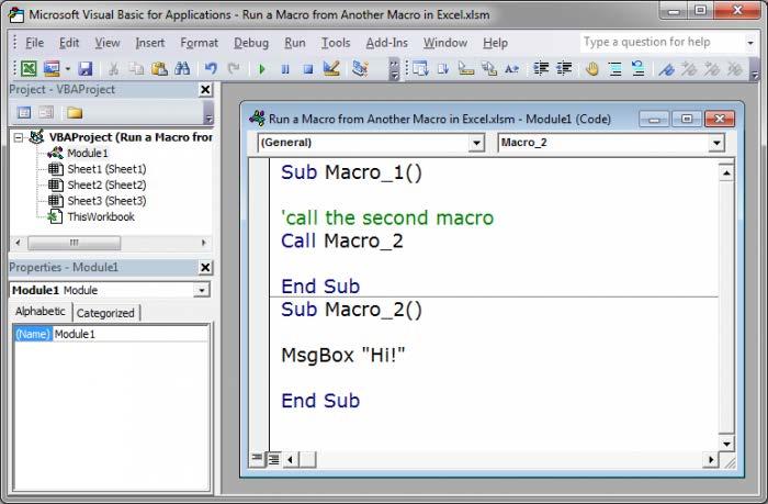
68 Run a Macro from Another Macro in Excel Download the Excel file for this tutorial (link will be in the side bar or at the bottom of the page) I will show you how to run a macro from another macro in Excel. This means that you can run any macro when you need to from a completely separate macro. This is actually very simple! Use Call in VBA. Here is the macro we want to call or run using another macro: Sub Macro_2() End Sub MsgBox "Hi!" And here is the macro that will call or run this macro: Sub Macro_1() End Sub 'call the second macro Call Macro_2 It is as simple as that. Put Call in front of the name of the macro that you want to run. Here is a screenshot of these two macros in Excel:

69