A Performance Evaluation of RPL in Contiki

Transcription

1 Master s Thesis Computer Science Thesis no: MCS A Performance Evaluation of RPL in Contiki A Cooja Simulation based study Hazrat Ali School of Computing Blekinge Institute of Technology SE Karlskrona Sweden i

2 This thesis is submitted to the School of Computing at Blekinge Institute of Technology, Sweden in partial fulfillment of the requirements for the degree of Master of Science in Computer Science. The thesis is equivalent to 20 weeks of full time studies. Contact Information: Author: Hazrat Ali Address: SICS, Stockholm Sweden External advisor: Simon Duquennoy, Ph.D Swedish Institute of Computer Science (SICS), Sweden. Address: SICS, Isafjordsgatan 22, Box 1263, SE Kista, Sweden Website: University advisor: Martin Boldt, Ph.D School of Computing, Blekinge Institute of Technology (BTH), Sweden Website: School of Computing Blekinge Institute of Technology SE Karlskrona Sweden Internet : Phone : Fax : ii

3 ACKNOWLEDGEMENTS This study has been carried out in collaboration with Swedish Institute of Computer Science (SICS) at Stockholm, Sweden. SICS is a leading research institute for applied Computer Science in Sweden. The Network Embedded System (NES) group at SICS focuses on research about wireless network systems and the internet of things. The WSN operating system Contiki and the Simulation tool Cooja used in this study have been developed at NES research group. I got the honor to work with these great researchers, founders and scientists and got inspiration and knowledge about research. I would like to express my special thanks to all the researchers in the NES group for their assistance during this study. I am very grateful to Adam Dunkels, Thiemo Voigt, Joakim Eriksson, Niclas Finne, Fredrik Österlind, Nicolas Tsiftes, and Niklas Wirström for not only accommodating my queries and tackling various issues but also filling me with inspiration for more improvements in the thesis. I am very thankful to my advisors Simon Duquennoy (SICS) and Martin Boldt (BTH), who supported and guided me throughout the thesis work and without their immense cooperation this would never has been come to a successful end. I am also thankful to Khalid Khan (Master student software engineering, BTH) for his time in critical reviewing and discussion on the thesis. I am most thankful to almighty Allah, for answering my prayers, for giving me the strength to plod along the whole way up to the end during this research work. iii

4 ABSTRACT A Wireless Sensor Network is formed of several small devices encompassing the capability of sensing a physical characteristic and sending it hop by hop to a central node via low power and short range transceivers. The Sensor network lifetime strongly depends on the routing protocol in use. Routing protocol is responsible for forwarding the traffic and making routing decisions. If the routing decisions made are not intelligent, more re-transmissions will occur across the network which consumes limited resources of the wireless sensor network like energy, bandwidth and processing. Therefore a careful and extensive performance analysis is needed for the routing protocols in use by any wireless sensor network. In this study we investigate Objective Functions and the most influential parameters on Routing Protocol for Low power and Lossy Network (RPL) performance in Contiki (WSN OS) and then evaluate RPL performance in terms of Energy, Latency, Packet Delivery Ratio, Control overhead, and Convergence Time for the network. We have carried out extensive simulations yielding a detailed analysis of different RPL parameters with respect to the five performance metrics. The study provides an insight into the different RPL settings suitable for different application areas. Experimental results show ETX is a better objective, and that ContikiRPL provides very efficient network Convergence (14s), Control traffic overhead (1300 packets), Energy consumption (1.5% radio on time), Latency (0.5s), and Packet Delivery Ratio (98%) in our sample RPL simulation of one hour with 80 nodes, after careful configuration of DIO interval minimum/doublings, Radio duty cycling, and Frequency of application messages. Keywords: RPL, Routing metrics, Cooja, Objective Function, Evaluation, Low Power and Lossy Network. iv

5 CONTENTS A PERFORMANCE EVALUATION OF RPL IN CONTIKI I ACKNOWLEDGEMENTS III ABSTRACT IV 1 INTRODUCTION PROBLEM STATEMENT AIMS AND OBJECTIVES THESIS STRUCTURE 11 2 BACKGROUND WIRELESS SENSOR NETWORK CONTIKI, A SENSORNET OPERATING SYSTEM COOJA SIMULATOR PROTOCOL STACK DUTY CYCLING OVERVIEW OF RPL TOPOLOGY FORMATION ROUTING IN RPL RPL MESSAGES ROUTING METRICS ROUTING CONSTRAINT OBJECTIVE FUNCTION TRICKLE TIMER HOW CONTIKIRPL WORKS 24 3 RELATED WORK 25 4 RESEARCH QUESTIONS RESEARCH QUESTIONS MOTIVATION 29 v

6 5 RESEARCH METHODOLOGY LITERATURE REVIEW EVALUATION MODELING RESULT ANALYSIS VALIDITY THREATS 32 6 EVALUATION PERFORMANCE METRICS RPL, DUTY-CYCLING, APPLICATION: PARAMETERS SIMULATION AND NETWORK SETUP LINK FAILURE MODEL NETWORK SETUP MEASURING THE PERFORMANCE METRICS MEASURING THE CONTROL TRAFFIC RUNNING THE SIMULATIONS PHASE 1: COMPARISON OF OBJECTIVE FUNCTIONS OF0 VS. ETX PHASE 2: RPL EVALUATION DIO MINIMUM INTERVAL DIO INTERVAL DOUBLINGS DUTY-CYCLING INTERVAL FREQUENCY OF APPLICATION MESSAGES 65 7 ANALYSIS OF THE RESULTS 71 8 DISCUSSION 75 9 CONCLUSION AND FUTURE WORK REFERENCES APPENDIX - A: RPL PACKET FORMATS APPENDIX - B: CODE SNIPPETS APPENDIX -C: FIGURES AND TABLES 91 vi

7 LIST OF FIGURES Fig. 2.1: Contiki Protocol Stack [3] Fig. 2.2: Sampled Listening Fig. 2.3: RPL Network Topology Fig. 2.4: DIO sent by root after RPL starts Fig. 6.1: The radio medium is simulated by UDGM Fig. 6.2: RPL Network Setup of 80 client nodes and 1 sink node Fig. 6.3: Timeline for DIO transmission using Trickle algorithm Fig. 6.4: Outline for running the automated simulation scripts Fig. 6.5: Latency comparison of OF0 and ETX in Contiki Fig. 6.6: Energy consumption for OF0 and ETX in Contiki Fig. 6.7: Packet Delivery Ratio of OF0 and ETX in Contiki Fig. 6.8: Network Setup Time for DIO Interval Minimum Fig. 6.9: Control Traffic overhead for DIO Interval Minimum Fig. 6.10: Energy Consumption for DIO Interval Minimum Fig. 6.11: Network Latency for DIO Interval Minimum Fig. 6.12: Packet Delivery Ratio for DIO Interval Minimum Fig. 6.13: Network Setup Time for DIO Doublings Fig. 6.14: Control Traffic overhead for DIO Doublings Fig. 6.15: The Percent Radio ON time for DIO Doublings Fig. 6.16: The Network Latency for DIO Doublings Fig. 6.17: The PDR for DIO Doublings Fig. 6.18: The Network setup time for Radio Duty Cycling Interval Fig. 6.19: The Control Traffic overhead for Radio Duty Cycling Interval Fig. 6.20: The Energy Consumption for Radio Duty Cycling Interval Fig. 6.21: The Network Latency for Radio Duty Cycling Interval Fig. 6.22: The PDR for Radio Duty Cycling Interval Fig. 6.23: The Packet Loss for Frequency of application messages Fig. 6.24: The Network Setup Time for Frequency of application messages Fig. 6.25: Control Traffic overhead for Frequency of application messages Fig. 6.26: The Energy consumption for Frequency of application messages Fig. 6.27: The Network Latency for Frequency of application messages Fig. 6.28: The PDR for Frequency of application messages Fig. 11.1: RPL DIO Packet Format Fig. 11.2: RPL DIS Packet Format Fig. 11.3: RPL DAO Packet Format vii

8 NOMENCLATURE DAO DIO DIS DODAG ICMP IEEE IETF IP LLN MAC OF RDC RPL TCP WSN Destination Advertisement Object DODAG Information Object DODAG Information Solicitation Destination Oriented Directed Acyclic Graph Internet Control Message Protocol Institute of Electrical and Electronics Engineers Internet Engineering Task Force Internet Protocol Low Power and Lossy Network Medium Access Control Objective Function Radio Duty Cycling Routing Protocol for LLN Transmission Control Protocol Wireless Sensor Network viii

9 CHAPTER ONE Introduction 1 INTRODUCTION The use of low-power wireless devices is becoming part of our daily life. It has many application areas like industrial automation, home automation, security, and the smart grid. The devices in sensor network are resource constrained because they are small, low power, and low cost. Since sensor nodes run on battery, which cannot be recharged, consequently it is vital that it runs very efficiently in terms of computation and communication. Computation activities, compared to communication are less power consuming. It is the communication activities of transmitting and receiving which take up most of the energy [1] [2]. Therefore it is essential to evaluate the resource consumption and efficiency of the routing protocol in these devices. The scarce resources also make them use short-range radios, which are vulnerable to interference with other devices in the vicinity. These networks are also termed as Low Power and Lossy Networks (LLNs). The devices in LLN are interconnected by a variety of links for instance Bluetooth, IEEE , Low Power Wi-Fi, or low power PLC (Power line communication). The nature of LLN is lossy because an increasing number of wireless devices like cordless phones. Microwave, Wi-Fi etc are deployed using the same spread spectrum bands (900MHz, 2.4GHz, and 5GHz bands), which interfere with the tiny motes in the vicinity. The physical obstacles between a sender and a receiver also disturb the devices in LLN or smart objects. Apart from this, wireless links have the problem of multipath fading, shading and hidden nodes etc. The more devices operate simultaneously within a small distance of each other the more degraded is the performance [3]. A lossy link is not just a link with high bit error rates but packet drops on lossy links are extremely frequent and the links may become unusable for quite some time due to interference [2]. To make use of the scarce resources in LLN efficient, resource-consuming activities need to be regularized. The most energy consuming part in LLN is the transceiver. 9

10 Chapter 1: Introduction Since a node in an LLN not only forwards its own packet towards the destination (sink for example) but also routes the packets of the other nodes in the network, therefore routing is of great concern in wasting the resources in these devices. An LLN contains several alternative paths towards a single destination but with different link qualities and reliabilities. It becomes the prominent liability of the routing protocol to make intelligent decisions in making the routes from a source to a destination. The poor path selection causes the scarce resources to drain out quickly. There are several application areas like industrial and home automation, urban and commercial buildings [4 6] which require data collection from different nodes in the network therefore the study focuses on Multipoint-to-point (M2P) network scenarios. 1.1 Problem Statement Routing is a crucial factor influencing connectivity and performance of information exchange. The general performance of Low Power and Lossy Network (LLN) is highly dependent on the choice of routing protocol and quality of its implementation. Since LLNs are very resource constrained therefore Control Traffic, Convergence Time, Energy consumption, Latency and Packet delivery ratio (PDR) play a vital role in performance of the routing protocol. Routing Protocol for Low Power and Lossy Network (RPL) need to be optimized for different sensornet applications to gain optimized performance and utilize the constrained resources more efficiently because each packet sent consumes resources worth noticing for a LLN network. 1.2 Aims and Objectives The overall aim of this thesis is to evaluate the performance of Routing Protocol for Low Power and Lossy Network (RPL) with respect to different performance metrics. The goal is to observe differences in behaviors and determining what causes they are resulting from. Detailed experimental outcomes and diagrams are meant to help account the alterations of network performance, as effects of tweaking different parameters related to RPL. Investigate the behavior of RPL over duty-cycled networks. 10

11 Chapter 1: Introduction Evaluating the performance of RPL with respect to Convergence Time, Control Traffic overhead, Energy consumption, Latency, and Packet Deliver Ratio (PDR). Evaluating the performance of the two implemented Objective Functions (OF) in Contiki (Sensornet OS). Find the impact of RPL and Contiki Parameters namely DIO Minimum Interval, DIO Doublings, Duty cycling, Frequency of application messages on the standard performance metrics of interest. The objectives of this thesis are: Carry out background study and literature review about the RPL protocol, Routing metrics and Objective functions. Analyze the behavior of RPL over duty cycled networks in COOJA simulator. Study various relevant IETF ROLL (routing over LLN) internet-drafts (RPL-19. Objective function, routing metrics. Trickle timer) and research articles. 1.3 Thesis Structure In the next chapter we describe the background of the field necessary to understand the concepts and terms in this study. The related work about the problem is summarized in chapter 3 and the research questions in chapter 4. In chapter 5 we present our methodology we adopted for this research to answer the research questions. The development section of the thesis starts in chapter 6 where we carry out the detail simulations and analysis. We present the results and outcomes from the simulations in the next chapter 7. The discussion of the research is given in chapter 8. Finally in chapter 9 we present the conclusion of the research and future research work generated from this study. 11

12 CHAPTER TWO Background 2 BACKGROUND 2.1 Wireless Sensor Network A wireless sensor network also called Low power and lossy network (LLN) is a class of networks consisting of devices with a communications infrastructure intended to monitor physical or environmental conditions at diverse locations. Commonly monitored parameters are temperature, humidity, pressure, power-line voltage, and vital body functions etc. The devices in a sensor network called sensor nodes are equipped with a transducer, microcomputer, transceiver and power source. The transducer generates electrical signals based on sensed physical effects and phenomena. The microcomputer processes and stores the sensor output. The transceiver transmits and receives radio signals, and power source provides electricity to these devices. The size of these devices is usually very small and powered by either battery, energy scavenging like solar cells or mains powered. The size factor of the devices also makes them resource constraint and therefore they need a very sensible use of the resources. LLNs are aimed for low traffic applications. Low traffic is very common for smart home applications, ubiquitous computing where a very long life is required. A wireless sensor network can support three types of traffic: Point-to-Point (between devices inside the LLN), Point-to-Multipoint (between the central device and other devices inside LLN), and Multipoint-to-Point (between the devices inside the LLN to a central device). Since the devices have limited range of transmission, therefore Routing is required in these devices to reach each other. Routing is responsible for managing the routes among sensor nodes and forwarding the packets on the most efficient route discovered. To send or receive these packets the nodes use the transceiver part which is a short range radio. The radio medium used by LLN devices is of short range and also very susceptible to bit errors. The lossy nature of LLN has a strong impact on the routing protocol design. Since the link failures are frequent and usually transient, therefore the 12

13 Chapter 2: Background routing protocol should not overreact in an attempt to converge the network as a result of temporary failures [7]. Due to these reasons, one of the challenging issues in wireless sensor networks is finding the best routes for the delivery of data, which implies a very efficient routing mechanism for finding and keeping the routes in the network. The routing mechanism is subjected to both the resource constraint nature of sensor nodes and lossy nature of the radio medium in LLN. 2.2 Contiki, A Sensornet Operating System Contiki is a wireless sensor network operating system and consists of the kernel, libraries, the program loader, and a set of processes [8]. It is used in networked embedded systems and smart objects. Contiki provides mechanisms that assist in programming the smart object applications. It provides libraries for memory allocation, linked list manipulation and communication abstractions. It is the first operating system that provided IP communication. It is developed in C, all its applications are also developed in C programming language, and therefore it is highly portable to different architectures like Texas Instruments MSP430. Contiki is an event-driven system in which processes are implemented as event handlers that run to completion. A Contiki system is partitioned into two parts: the core and the loaded programs. The core consists of the Contiki kernel, the program loader, the language run-time, and a communication stack with device drivers for the communication hardware [8]. The Program loader loads the programs into the memory and it can either obtain it from a host using communication stack or can obtain from the attached storage device such as EEPROM. The Contiki operating system provides modules for different tasks (layers). It provides the routing modules in a separate directory contiki/core/net/rpl and consists of a number of files. These files are separated logically based on the functionalities they provide for instance rpl-dag.c contains the functionality for Directed Acyclic Graph (DAG) formation, rpl-icmp6.c provides functionality for packaging ICMP messages etc. In this study most of the work is related to these files of the Contiki operating system. 13

14 Chapter 2: Background 2.3 Cooja Simulator Cooja is a Java-based simulator designed for simulating sensor networks running the Contiki sensor network operating system [9]. The simulator is implemented in Java but allows sensor node software to be written in C. One of the differentiating features is that Cooja allows for simultaneous simulations at three different levels: Network Level, Operating System Level and Machine code instruction level [9]. Cooja can also run Contiki programs either compiled natively on the host CPU or compiled for MSP430 emulator. In Cooja all the interactions with the simulated nodes are performed via plugins like Simulation Visualizer, Timeline, and Radio logger. It stores the simulation in an xml file with extension 'csc' (Cooja simulation configuration). This file contains information about the simulation environment, plugins, the nodes and its positions, random seed and radio medium etc. Cooja Simulator runs the Contiki applications whose files are placed in another directory and may also contain a project-conf.h file which provides the ability to change RPL parameters in one place. 2.4 Protocol Stack Traditional TCP/IP implementations need too many resources both in terms of code size and memory usage which is not useful for smart objects with limited resources [10]. The WSN TCP/IP stack is designed to have only the absolute minimal set of features of a full TCP/IP stack. The WSN protocol stack has four layered architecture as shown in Figure 3.1. These layers are explained below and excerpted from [2]. Application Transport Network MAC and Physical HTTP, Telnet UDP, TCP IP Communication Driver ICMP Device Fig. 2.1: Contiki Protocol Stack [3] 14

15 Chapter 2: Background 1. Physical and MAC Layer This layer defines the physical characteristics of the network such as frequency, timing and voltage etc. The physical layer use different communication mechanism like IEEE , IEEE and Power Line Communication (PLC) etc but here we will explain only as it is used on low power and lossy networks and related to this study. IEEE is a relatively short range transmission mechanism whose range is only a few meters and is a standard radio technology for low power networks [2]. IEEE uses three different frequency ranges because of different regulations in different parts of the world. For United States it uses MHz, for Europe it uses MHz and for the rest of the world it uses MHz. The rates vary from 20 to 250kbit/s depending on the frequency. The IEEE standard also specifies MAC layer. IEEE supports two MAC addressing formats: long (64 bit) and short (16 bit). IEEE uses two types of modulation: binary phase shift keying (BPSK) and quadrature phase shift keying (QPSK). The maximum frame size is 128 bytes including the (1 Byte) MAC header [11]. 2. Network Layer This layer provides routing decision and forwards packets from node to node. On network level of the protocol stack is RPL protocol used for routing and forwarding of packets. The RPL protocol make use of control packets (DIO, DIS, DAO) for building a tree like topology and maintaining routes. The control packets also carry information about different parameters of the network. This layer forwards a packet if the destination address does not match any of node's unicast or multicast addresses. The layer will forward the packet to another node either because the packet is destined for it or that node has a route to the destination. IPv6 is better suited to the needs of WSN than IPv4. IPv6 require some adaptation to better support operation in WSN, which can be easily found in IPv6 s support for a simple header options. The structure of IPv6 addresses is also more amenable to cross-layer compression. The inclusion of necessary functionality required for sensor network nodes like DHCP, packet forwarding, auto configuration and routing have been incorporated in IPv6 [12], [13]. 3. Transport Layer This layer has two protocols UDP and TCP. This layer first recalculates the checksum to make sure that the packet is valid and then using its port number 15

16 Chapter 2: Background delivers the packet to the application. In case of TCP this layer also check its port number against list of active connections before passing it to the application. If a connection does not exists it then checks the list of listening TCP ports provided the packet has TCP SYN flag set. It will then create a new entry in the list of active TCP connections and deliver the packet to the application. 4. Application Layer This layer provides the API for applications to use the services offered by the lower layers. This layer has the applications like http, telnet etc. 2.5 Duty Cycling Duty Cycling is the technique of keeping the radio off as much as possible and switch it on only when needed. The WSN devices are small and operate with very small batteries that provide power for only a very limited time. However, duty cycling can significantly reduce Energy Consumption. Now-a-days a duty cycling protocols of less than 1% duty cycling is being proposed [14 16]. Idle listening refers to the process of keeping the radio on and listens to idle channel, and waiting for a potential packet to arrive. But idle listening is very expensive in terms of energy and consumes at least as much energy as while receiving [1]. There are two techniques of duty cycling, sampled listening and scheduling [12], [17]. In sampled listening the channel is monitored periodically to determine if a frame is being transmitted by its neighbor node. A node keeps on transmitting the frame in order to lengthen the transmission time to be as long as the receiver's sample period. Fig. 2.2: Sampled Listening For instance ContikiMAC uses sampled listening as shown in Figure 3.2, node 3 wants to send a packet to node 2. Node 3 keeps on sending this frame continuously (depending on the frame size and duty cycling interval) until node 2 awakes and receives the frame. 16

17 Chapter 2: Background In sampled listening the nodes do not need to keep state information to communicate. While in scheduling the nodes keep state information about the schedules of the neighbor nodes. The sending node knows from this information when the receiver's node is listening. Scheduling eliminates the need for sending the frame several times but at the cost of maintaining state information. 2.6 Overview of RPL A routing protocol is responsible for forwarding the packets from other nodes and making intelligent routing decisions. There are two types of routing protocols in WSN: Reactive and Proactive [18]. The reactive protocols provide routes when needed. Therefore it decides if a route is needed from the mobility of data by flooding its query in the network. These types of protocols (AODV [19], DSR, and TORA [20]) confine Control Traffic and transmit it when required by the path of data transfer. However this increases the time required for finding the routes when needed by the data. Whereas the proactive routing protocols provide the routes before it is actually needed by any data or node. Therefore these protocols periodically exchanges control messages to find and propagate the routes in the network as soon as they start. Nodes send both local control messages to share local neighborhood information; and messages across the entire network for sharing the topology related information among all the nodes in the network. Routing protocol for low power and lossy networks (RPL) is IPv6 routing protocol for low power and lossy networks designed by IETF routing over low power and lossy network (ROLL) group [7] as a proposed standard. RPL is distance vector protocol because linked state protocols require a significant amount of memory (links state database, LSDB) which is not suitable for the resource constrained LLNs. RPL is a proactive routing protocols and start finding the routes as soon as the RPL network is initialized. RPL forms a tree like topology also called DAG. Each node in a RPL network has a preferred parent which acts like a gateway for that node. If a node does not have an entry in its routing table for a packet, the node simply forwards it to its preferred parent and so on until it either reaches the destination or a common parent which forwards it down the tree towards the destination. The nodes in a RPL network have routes for all the nodes down the tree. It means the nodes nearer to the root node have larger routing tables. Route aggregation is not recommended because of several problems in LLN like mobility of nodes and more losses in the radio medium. 17

18 Chapter 2: Background Path selection is an important factor for RPL and unlike traditional networks routing protocols, RPL uses more factors while computing best paths for example routing metrics, objective functions and routing constraints. These factors are described in detail in the following sections. RPL uses TCP/IP for communication as it is has become a global standard after the success of internet. IP is used in LLN to provide end to end connectivity. It also solves the problem of interoperability between these devices from different vendors [21], [22]. It also facilitates the development of applications and integrations in terms of data collection and configuration [23]. Experience has shown that IP is both lightweight enough to run on even severely resource constrained systems [13]. In the following sections we describe RPL topology, routing mechanism, RPL control messages, routing metrics, constraints, Objective functions, Trickle timer and finally an example about RPL working Topology Formation LLNs do not typically have predefined topologies, for example those imposed by point to point wires, so RPL has to discover links to form a topology first. Figure 2.3: RPL Network Topology RPL creates a tree like topology with a root at the top and leaves at the edges as shown in Figure 2.3. In contrast to tree topology, RPL offers redundant links which is a MUST requirement in LLN [7], so actually violating the actual tree topology. RPL uses "up" and "down" direction s terminology regarding the movement of traffic. The up is from the leaves to the root and down from the root to the leaves. A typical RPL topology is shown in figure Routing in RPL RPL is a distance vector protocol and the operation of the protocol can be divided into two main phases. 18

19 Chapter 2: Background 1. Routing upward 2. Routing downward The topology information is maintained in Destination Oriented Directed Acyclic Graph (DODAG). The DODAG contains the paths from the leaves to the root. The root, which is also called an LLN border router (LBR), may be connected to a non-lln network, such as a private network; in which case the DODAG is considered to be grounded. 1. Routing Upward In order to route the traffic upward, RPL only need the information in the DODAG. The DODAG tells who the preferred parent of the node is. So when a node wants to send a packet to the root, it simply sends the packet to its preferred parent in the tree, and the preferred parent then sends the packet to his preferred parent and so on until the packet reaches the root. The rank is used to determine the relative position of a node in the DODAG and is used for loop avoidance as well. The rank is computed according to the OF. The rank is a 16bit monotonic scalar and is always higher than the rank of any of the parents. The RPL protocol populates DODAG with the parent information. The DODAG uses control packets called DODAG Information Object (DIO) and DODAG Information Solicitation (DIS) to convey the DODAG information. The formation of the DODAG is governed by the following rules [2]. 1. The path metrics. 2. The Objective Function (OF) 3. The policies of the node. 4. Rules used for loop avoidance which is based on DODAG ranks. A RPL instance identified by RPLinstanceID may contain several DODAGs identified by DODAGID. Different DODAGs are necessary for steering different types of network traffic [2]. Each DODAG has its own OF, metrics and sink. The DODAG uses DODAGSequenceNumber to show the freshness of the information. A DODAG is uniquely identified by the combination of RPLinstanceID and DODAGID. While a DODAG iteration is identified by the tuple RPLinstanceID, DODAGID and DODAGSequenceNumber. The DODAG building process is explained in the following steps. Step 1: The network administrator configures (at application level) one or more nodes as a DODAG root (node 1 in Figure 2.3). The DODAG roots starts sending 19

20 Chapter 2: Background the link local multicast DIO messages. A node may also solicit for DIO from the root in the mean time using DIS, in which case the DODAG root will send the DIO immediately. Step 2: The nodes nearby (node 2, 3 in Figure 2.3) will receive the DIO from the root and will process it as it is from a lower rank node and will select root as their parent. Step 3. These nodes will now send link local multicast DIOs and the other nodes (e.g. nodes 4,5,6,7 in Figure 2.3) receiving the DIO may select them as parent. If a node receives DIOs from two or more parents, it will decide based on the OF (e.g. optimize path ETX, or prune battery operated nodes etc). This process will continue until all the nodes join the DODAG. 2. Routing Downward RPL uses DAO messages to maintain the routing table in support of downward traffic. Although the term refers to "downward" direction but the DAOs are always sent upward. This makes RPL a hierarchical network in terms of control messages flow. The DAOs can only be sent after the topology formation (or DODAG creation) by the exchange of DIOs control messages. The IP architecture proposed by IETF ROLL separates the forwarding task from routing. The task of the forwarder is to receive datagrams and forward it to the suitable interface based on the routing table. The router is responsible for populating and maintaining routing table RPL Messages RPL uses three types of control messages for creating and maintaining RPL topology and routing table. These messages are: DODAG Information Object (DIO), DODAG Information Solicitation (DIS) and DODAG Destination Advertisement Object (DAO). 1. DODAG Information Object (DIO) DIO messages are used by RPL to form, maintain and discover the DODAG. When a RPL network starts, the nodes start exchanging the information about the DODAG using DIO messages which contains information about the DODAG configuration and help the nodes to join the DODAG and select parents. 2 DODAG Information Solicitations (DIS) 20

21 Chapter 2: Background The DIS is used by any node to explicitly solicit the DIO messages from the neighbor nodes. It is triggered by the node in case when it could not receive a DIO after a predefined time interval. 3. DODAG Destination Advertisement Object (DAO) The DAO messages are used by RPL to propagate a node prefix to the ancestor nodes in support of downward traffic Routing metrics A routing metric is a quantitative value used to find the cost of a path and helps in making the routing decision in case there are different routes available. In LLN a metric is a scalar used to find the best path according to the objective function. Routing metrics are a critical component to the routing strategy. Most of the IP routing protocols such as OSPF and IS-IS used in traditional network use static metrics (interface bandwidth) or some static value based on interface speed for instance. But LLN has a wide variety applications and constraints which strongly appeal for dynamic metrics. To better understand the need of dynamic metrics and difference between a metric and constraint for LLN, let's consider the following examples. 1. An application requires a quick delivery of packets using a short path and therefore the goal will be to use ETX metric for routing. 2. An application may require encrypted communication and therefore the goal will be to avoid non-encrypted links in the path. 3. A node may be energy constrained and the objective will be to minimize Energy Consumption by using as many mains connected nodes along the path as possible. In the first example the ETX is a routing metric. In the second example in which the goal is to avoid non-encrypted links; can be considered as a constraint which is explained next. In the third example energy can be either a constraint in which case the path will not contain any battery operated node or it can be a metric in which case the path may contain the minimum number of battery operated nodes as compared to the alternate paths. Unlike traditional networks LLN also use node metric apart from link metrics. Therefore the metrics can be categorized as node metric and link metrics as stated below [24]. 21

22 Chapter 2: Background Node metrics: Node State Attribute (NSA), Node Energy, Hop count Link metrics: Throughput, Latency, Link Quality Level, ETX, Link Color ContikiRPL implements two routing metrics, hop count and ETX. Hop Count: This metric counts the number of hops from the source to the destination. A hop count of 3 means there are 3 intermediate links between the source and destination. Expected Transmission Count (ETX): ETX of a link is the expected number of transmissions required to send a packet over that link. The path ETX is the sum of the ETX of all the links along the path. The ETX of a path with 3 links of 100% delivery ratio is 3, whereas the ETX of a path with 2 links of 50% delivery ratio is 4. Since low power networks have vastly varying requirements and characteristics like lossy links, resources constraints, mobility, a vast variety of applications, therefore RPL does not define any specific metrics or forwarding polices [7] and these are described in other IETF Drafts Routing Constraint A constraint is used to either include or exclude links from the routing path that do not meet the criteria specified in the objective function Objective Function An objective function (OF) defines how a RPL node selects and optimizes routes within a RPL instance based on the information objects available. Consider a physical network made of several links with different qualities such as throughput, Latency and nodes with different qualities such as battery operated, mains-powered. If the network carries different types of traffic it might be useful to carry the traffic based on different OFs which are optimizing different metrics or fulfilling constraints. Thus the OF is used to steer the traffic to different paths according to the requirements. These requirements are actually encoded in a programming logic what we call OF and used by RPL during routing operations which is explained next. ContikiRPL implements two OFs i.e. OF0 and ETX. OF0 uses hop count as routing metric where as ETX uses ETX metric as a routing metric for selecting the best path. 22

23 Chapter 2: Background This separation of OFs from the core protocol specification allows RPL to be adopted to meet the different optimization criteria required for a wide range of deployments, applications and network designs [7] Trickle Timer To save energy the DIOs are sent periodically controlled by the trickle timer whose duration is doubled each time it is fired. The smallest possible interval between two DIOs is equal to DIO Minimum Interval which keeps on increasing (doubling) until it reaches the maximum value determined by DIO Interval Doublings. There are three configurable parameters in the Trickle Timer: Imin, Imax and redundancy constant k [25] and explained below. 1. Imin This parameter gives the minimum amount of time between two DIOs. DIOs are transmitted periodically to reduce the redundant Control Traffic and use the limited resources more optimally. The transmission of DIO is controlled by a timer called trickle timer whose minimum value is Imin and maximum value is Imax. The value of trickle timer starts from the lowest possible value Imin and is doubled each time it is transmitted until it reaches its maximum possible value of Imax. The value of Imin is determined by the RPL parameter DIO Minimum Interval (In Contiki: RPL_DIO_INTERVAL_MIN) and computed as: Imin = 2 ^ RPL_DIO_INTERVAL_MIN So if RPL_DIO_INTERVAL_MIN = 12 then Imin = 2 ^ 12 = 4096 ms = 4 s. This is the smallest interval between two DIOs provided RPL_DIO_INTERVAL_MIN equals Imax This parameter is used to limit the number of times the Imin can be doubled. The value of Imax is determined by the RPL parameter DIO Interval Doublings (In Contiki: RPL_DIO_INTERVAL_DOUBLINGS) and computed as: Imax = Imin * 2 ^ RPL_DIO_INTERVAL_DOUBLINGS..(3.a) So if RPL_DIO_INTERVAL_DOUBLINGS = 8 and Imin is 4096 then Imax = 4096 * 2 ^ 8 = ms = 17.5 min. This is the maximum time between two successive DIOs required under a steady network condition. 23

24 Chapter 2: Background 3. Redundancy constant (k) It is a natural number greater than 0 and is used to suppress the DIO transmission How ContikiRPL Works A typical ContikiRPL network in Cooja simulator is shown in Figure 3.3. The root node or LLN Border Router (LBR) located at the top of the topology tree has a node id 1. When the RPL network starts, the root of the DAG starts sending out the DIO messages to let the neighbors know the parameters of the network like DAG-ID, OF, routing metric, rank etc as shown in Figure 2.4. The LBR is set by the administrator in advance as a root and has rank equal to 1. Fig. 2.4: DIO sent by root after RPL starts Once the nearby (child) node (for instance node 2 in Figure 2.3) receives a DIO, it calculates its rank based on the parent rank and its cost of reaching the parent node. The node follows a set of rules for parent selection (as explained in the previous section like OF, metrics). Any node with a lower rank is considered as a candidate parent and is added to candidate parent list by RPL. When the node joins the DAG after the reception of DIO it sends out all the information like DAG-ID, OF, routing metric, rank etc so that other nodes ( say node 4 in Figure 3.3) will receive it in turn and will join the DAG after calculating its rank. This process continues down until the farthest node in the topology tree joins the DAG. If a node does not receive a DIO for more than an interval of 5 seconds it sends a DIS message and nodes receiving DIS will send DIO promptly. Once the node selects its parents and hence form the topology for upward traffic it then starts sending DAO (to its parent) to advertize its prefix. The node (parent) that receives DAO updates its routing table hence enabling downward traffic. 24

25 CHAPTER THREE Related Work 3 RELATED WORK Routing in LLN is challenging not only because of lossy nature of the radio medium and the constrained resources of the sensor nodes but also due to the various routing requirements and high flexibility of the RPL configurations. A variety of RPL metrics were used in the previous studies to evaluate its performance in various network scenarios and it has been observed that a number of optimizations can be added to a RPL network. One of the important tasks of a routing protocol is to find the shortest possible path to destinations and saving it in its routing table. The routing table size is usually measured in number of routing entries instead of Kbytes. RPL can work in both storing and non-storing mode and this enables very resource constrained nodes (with no memory for routing table) to join a RPL network [2]. In nonstoring mode a node is not required to store the routing entries in its routing table and source routing is used to carry the routing information along the path. The routing information is contained in the source routing header which is limited to 136 Bytes and so a maximum of 8 hops from source to destination is possible [26]. However 64 hops are possible in source routing header if address compression is used [27]. The size of the source routing header increases linearly with increasing length of the source route in both cases of either using or not using address compression [28]. A RPL node stores the routes to all the routes downward in the tree and the size of the routing table can use more memory in large networks assuming storing mode. However these path entries depends on the OF in use because each use different strategies and metrics to find the best path. In a sample network of 86 nodes 90% of the nodes will store only 21 routing entries and it reflects the best path selection by OF ETX [29]. In storing mode RPL computed paths are not very close to the hypothetical ideal paths in some scenarios where the sink is situated at one end of the network [29]. Comparing the paths along the DAG to the shortest possible paths, RPL computed paths along the DAG is longer which increase packet loss and delay [30]. In a network containing 100 to 1000 nodes the average number of hops selected by 25

26 Chapter 3: Related Work RPL per node is between 2 to 10 to the sink using hop count routing metric and grows logarithmically with the number of routes in the network [28]. Control Packet Overhead is an important characteristic of a routing protocol and directly relates to Energy Consumption. To control the generation of redundant control packets and utilize the scarce resources of LLN more efficiently RPL make use of Trickle Timer [25] which periodically transmits Control Traffic. When a RPL network starts the transmission of control packets is more but it starts dropping as soon as the network stabilizes [29], [31]. A RPL implementation in Omnet++ provides negligible Control Traffic overhead compared to data traffic in a loss free environment [29]. However some results [31] show that RPL Control Traffic overhead oscillates around 25% of the overall traffic with a small packet error rate (0.01) in a steady network of 20 nodes and the situation becomes more worse in a larger network of 100 nodes and the overhead raises between 30 to 75% of the overall traffic. The main reason of this large overhead is support of downward routing using DAOs because DIOs are transmitted locally whereas DAOs are transmitted up to the sink [31]. The Control Traffic overhead does not depend on data traffic however and it is two orders of magnitude higher than the other contemporary routing protocols for instance LOAD (A derivative of Ad-hoc on Demand Distance Vector Routing, AODV) [28]. The throughput (amount of data received at sink) of a RPL network fluctuates and depends on several aspects including the size of the network for instance a network of 20 and 100 nodes provides a throughput of about 50 Bytes and 200Bytes respectively. In case of individual nodes throughput the nodes closer to sink receive more data than the nodes closer to the leaves because the nodes in a RPL network not only forwards its own data but also support other nodes to reach their data to the sink [29]. RPL provides nearly 100% packet delivery ratio unless there is radio collision or packet loss [28]. The RPL fast Convergence Time is realized in many studies and is between 7 to 30 second in a network of 100 to 1000 nodes and it increase with the number routes in the network [28]. The article [32] presents a survey on routing protocols in wireless sensor networks. These protocols are divided into 3 categories namely data-centric, hierarchical and location-based. Data-centric based protocols name the data and query the nodes based on attributes of the data. This paradigm enables to avoid the overhead of forming clusters but these attribute based naming might not be useful for complex queries. Hierarchical protocols use data aggregation and fusion in order to decrease the number of transmitted messages to the sink. These protocols form clusters of the sensor nodes based on the received signal strength and use the 26

27 Chapter 3: Related Work cluster head for routing to the sink node and therefore provide greater scalability. The location based protocols use the location information and topological deployment of sensor nodes in support of energy efficient routing. Further this article has classified several routing protocols into the proposed categories. The packet delivery ratio can be used as a metric for selecting best paths by a routing protocol. There are three methods for calculating the packet delivery ratio in WSN [33]. In the first method a number of hello messages are sent to a sink and the number of successfully received packets is count at the sink. This method is accurate but consumes more energy. In the second method takes into account the PDR history and therefore energy efficient but lacks high accuracy. A third method of taking the advantage of the received signal strength and Exponential Weighted Moving Average into account computes path by 25% more accurate than the previous ones [33]. There are several application areas of LLN, which require both low and high data transfer rates and some techniques like burst forwarding, which groups multiple data packets, store them on flash memory and forwards them to the next hop [34]. This technique improves throughput and uses scarce resources of LLN for example energy more efficiently. All the studies stated above lacks the evaluation of RPL with respect to tweaking its own parameters for instance DIO interval, Duty Cycling interval, etc which plays a vital role in network convergence, Control Traffic overhead, and Energy Consumption. 27

28 CHAPTER FOUR Research Questions 4 RESEARCH QUESTIONS 4.1 Research Questions We have formulated the following main research question for this study. RQ. How does the performance of a RPL network vary with respect to different parameters? To answer this question we need to first define the metrics for network performance and secondly find the parameters that affect RPL performance. We evaluate RPL performance in terms of five metrics: energy, Latency, Packet Delivery Ratio, Control Traffic and network Convergence Time. Since RPL uses objective functions to select the best path therefore we need to evaluate first the two objective functions i.e. OF0 and ETX. This evaluation will enable us to evaluate the performance of RPL for the specified metrics with preferred OF. Next we define the parameters of RPL more influential on its performance. We use a systematic approach to evaluate the impact of each parameter on performance metrics. Consequently we shape the above general research question into the following more specific research questions. RQ1. What is the performance comparison of OF0 and ETX? RQ2. What is the impact of different RPL parameters on its performance with respect to Energy, Latency, Packet Delivery Ratio, Convergence Time and Control Traffic? 28

29 Chapter 4: Research Questions 4.2 Motivation The RPL is a new protocol just standardized by the IETF and under implementation stages. Its evaluation is useful to get insight and discover weaknesses in to the protocol and possibly to improve them in the future work. The specification of the protocol [7], [24], [25], [35] lacks the exact details of any implementation therefore implementation may exhibit a bad performance if not implemented carefully [36]. Due to these reasons evaluation is extremely necessary to find out the pros and cons of the protocol design and implementations. Since link layer technologies (IEEE , etc) vary in their properties the RPL protocol needs to be configured and optimized for each. It is important to evaluate the implementations of RPL for different link layer technologies and different environmental conditions (losses, interference, energy etc). This point also leads to a research question of what will happen if sensor nodes have different OS with different implementations of RPL. An agreed up on set of parameters optimized for the specific network will be required to address the issue. Some studies [29], [31] have evaluated RPL for point-to-point and multipoint traffic and different level of losses. An evaluation of Path ETX, Routing Table size, control overhead and loss of connectivity have been performed. Traffic of only 20% has been destined for sink which cannot justify for RPL performance for upwards traffic which is the focus of our study. Most of the applications in a WSN required the flow of data from sensor nodes towards a sink therefore upward traffic efficiency is very important for LLN. Furthermore a number of architecture oriented metrics like routing table size has been considered during the study however it lacks the performance mainly focused on the network traffic. The article [28] presents a comparison of RPL and LOAD (derivative of Ad-hoc on Demand Distance Vector Routing, AODV) protocols with respect to different network sizes. The article presents ns-2 simulation based results for standard evaluation metrics like average rank of routers, Network Convergence Time, Path Length etc. However RPL has evaluated in non-storing mode and without losses in the radio medium using b radio interface and therefore lacks simulating the real sensor network. This article also lacks the evaluation with respect to Energy Consumption because it could not be quantified using simulated nodes. However we are using a novel technique of software based online energy estimation for the sensor nodes called Powertrace [17], [37]. The LLN has several application areas that require both low data rate traffic and high throughput data transfers [34]. It is important to evaluate the RPL performance for 29

30 Chapter 4: Research Questions application messages. The design of the protocol is influenced by many challenging factors like Energy Consumption, network topology, network size, fault tolerance, and Latency etc. It is of great importance to evaluate RPL performance for these factors in order to effectively suggest its performance for specific area and use cases. 30

31 CHAPTER FIVE Research Methodology 5 RESEARCH METHODOLOGY We have carried out the research in a systematic way, in order to ensure its repeatability and validity. We have done the research in three main phases. In the first phase we have carried out a background study and literature review of the state of the art protocols and operating system for LLN. We also studied the different techniques available in Cooja simulator to analyze the results from simulation and the influential reasons. In the second phase we performed several simulations as the study is empirical. We have studied the impact of several parameters on RPL performance. We determined the critical metrics necessary for the performance evaluation of the routing protocol. This phase also include the selection of simulation tools followed by reporting and documenting process. We chose simulation for this study because it provides full control over all network parameters and full visibility into the network. In the third phase we analyzed the outcome of the results and present the conclusion. These phases are explained in their respective sections. 5.1 Literature Review A literature review is a means of evaluating and interpreting all available research relevant to a particular research question, or area. Its main aim is to present a fair evaluation of the research area of interest by conducting a rigorous and auditable methodology [38]. The main purpose of my literature review is to find the relevant literature about ContikiRPL for the purpose of background study, summarize the existing work and identify the gap in the current research. We searched the online research databases like IEEEXplore, ACM, Scopus, and Google Scholar. We present detailed Literature review in Chapter 3. 31

32 Chapter 5: Research Methodology 5.2 Evaluation Modeling After the initial phase of the background study and literature review we found that RPL has been designed with a great deal of flexibility because of the vast number of applications. It supports a variety of metrics [24] based on several OFs. It is necessary to evaluate OFs first and after that to evaluate RPL performance in terms of performance metrics for one preferred OF. To limit the scope of this study we left the evaluation of RPL with other OFs as a future work. After the initial phase a set of research questions was formulated as stated in section 1.3. As a result we need experimentation in order to find suitable answers to the research questions and addressing the research issues. For the purpose of evaluating the network performance, we modeled a simulated functioning network suitable enough for the observations of the performance metrics. We use simulations for this study firstly because it provides finer control on the rate of losses and other parameters. Secondly this study comprises extensive iterations of the simulations for several parameters; therefore simulation is more suited for repeatability of the simulations than test beds. For the sake of simulations we choose Cooja simulator which is the most widely used and the only available simulator for the Contiki Operating System. 5.3 Result Analysis We performed the analysis based on experimental results from simulation and the literature review. The literature review provides an insight into the previous studies and also helps us find the influential RPL parameters. The objective of analysis is to observe the impact of different RPL parameters on its performance with respect to metrics like Latency, Energy Consumption etc and to observe differences in behaviors and determining what causes they are resulting from. 5.4 Validity Threats Validity states that how much the research study and investigations are scientifically correct and insure that all research produce valid conclusions. Its primary purpose is to eliminate the more confounding variables to increase the accuracy and usefulness of findings [39], [40]. There are four types of validity and its associated threats which may introduce a variety of extraneous factors which causes intervention on the experiment and thus deteriorating the accuracy of the results [39]. 32

33 Chapter 5: Research Methodology i. Internal Validity Internal validity ensures that the independent variable was directly responsible for the effect on the dependent variable. Internal validity is thus controlling the internal parameters in the experiment for having any effect on the results. To overcome internal validity threats we studied the core concepts in the experimental designs, in depth study of the simulation tools, the start of the art research articles to see the factors that can influence our performance metrics in the experiment. It is also one of the reasons that we use Simulation which provides strong experimental control and as a result increases the overall internal validity. ii. External Validity External validity refers to the extent to which the results can be generalized beyond the study sample to other populations across time or other conditions, settings and circumstances. The external validity threats include experimental arrangements, environmental conditions, test sensitization and timing of measurement. Since WSN uses low power radio, external factors like Wi-Fi interference can cause more losses in the network than expected. To overcome this validity threat we use simulation in Cooja which provides accurate measurement and interference from other radio is avoided in a simulation environment. The simulation environment is usually ideal and provides better results than the unexpected environmental effects (novelty effects) but to simulate the network correctly and provide a valid evaluation of the protocol the external unexpected interferences are required to be omitted. Thus we limit the radio interference and collisions among and from the sensor nodes itself in the experiment. Also we administer one independent variable at a time in every experiment to eliminate the effect of one independent variable on the other (problem of multi-treatment interference). The Simulation of lossy medium is emulated by using the Cooja feature Unit Disk Graph Model (UDGM) and may not simulate the precisely the real network lossyness. However the simulation confirms the functionality and behavior of the routing protocol. The devices in a wireless network can be mobile or fixed depending on the applications and deployment. This study is valid for sensor network with fixed nodes only. Mobility in nodes may give different results because mobility needs rerouting of packets. To address this issue we limit the study to upward traffic. The upward traffic is used mostly in static environments of a sensor network. 33

34 Chapter 5: Research Methodology iii. Construct Validity Construct validity refers to the adequate definitions and measure of variables to accurately model the hypothesis. It ensures that the theory supported by the findings adequately provides the best explanation of the results. To overcome this validity threats we clearly define our independent and dependent variables in the relevant sections to improve construct validity [41]. The IETF drafts used during this study is continuously in progress. The IETF drafts are the documents valid for six months, therefore they are upgrading continuously. The description and functioning of different protocols, objective functions, metrics and other terminology may not conform to the older drafts. We have used the latest drafts available and the study is valid for the drafts mentioned in the reference section. iv. Statistical Validity Statistical validity refers to the statistical accuracy of the results drawn from the study. It asks the question if the results drawn are reasonable. Statistical validity threat may arise from variability in methodological procedures, low statistical power, and multiple error rates. We study different statistical methods in detail to decrease the validity threat. 34

35 CHAPTER SIX Evaluation 6 EVALUATION In this section we first evaluate OF0 and ETX in terms of performance metrics of interest. Later we configure a number of RPL parameters (DIO Minimum Interval and Doublings, Duty cycling interval, Frequency of application messages) to observe their cause and effect on performance metrics of interest. A number of protocol parameters influence the efficiency of RPL; the four significant among them are DIO minimum interval, DIO Doublings, Radio Duty Cycling interval and Frequency of application messages. To observe the effect of these parameters on ContikiRPL performance we use five performance metrics of interest: Convergence Time, Control Traffic overhead, Energy consumption, Network Latency, and Packet delivery ratio (PDR). In the first phase of the simulations we evaluate the performance of OF0 and ETX in terms of three metrics: Energy consumption, Network Latency and Packet delivery ratio to propose an efficient Objective function. In the second phase we evaluate RPL in terms of five metrics of interest stated above for the preferred OF suggested at first phase. In the rest of the chapter we describe the performance metrics of interest in section 6.1, that we will use to observe the performance of RPL after changing the parameters. The parameters that impact RPL performance are described in section 6.2. In section 6.3 we describe the Link failure model which is used to simulate the lossy radio medium in Cooja. We perform the simulations in phase 1 and phase 2 in sections 6.4 and 6.5 respectively. 35

36 Chapter 6: Evaluation 6.1 Performance metrics We use five standard performance metrics namely Network convergence, Control Traffic overhead, Energy consumption, Packet Latency and PDR to evaluate the performance of RPL. The first performance metric of interest is Network Convergence Time. The nodes in a sensor network need to form a topology in order to communicate. Therefore the network setup time is a crucial metric that need to be evaluated for any routing protocol. The Convergence Time of the RPL DAG is defined as the amount of time needed by all the reachable (in terms of radio) nodes in the network to join the DAG. This convergence should be considered as the initial Convergence Time in a RPL network with static nodes. As the nodes can be mobile and the links are lossy in LLN, the absolute Convergence Time cannot be defined for a mobile network. The second performance metric is Control Traffic Overhead for the network. This includes DIO, DIS and DAO messages generated by each node and it is imperative to confine the Control Traffic keeping in mind the scarce resources in LLN. RPL control the redundant control messages by making use of trickle timers. The aim of this metric is to analyze the effect of the stated parameters on the Control Traffic overhead. The third performance metric is Energy Consumption. To make good energy estimation we use percent radio on time of the radio which dominates the power usage in sensor nodes. Furthermore we take the average percent radio on time for all the nodes in the whole network setup. The fourth performance metric of interest in the study is Packet Latency. The Latency is defined as the amount of time taken by a packet from node to reach the sink and is the average of the latencies of all the packets in the network from all the nodes. The fifth metric is Packet Delivery Ratio (PDR) and is defined as the number of received packets at the sink to the number of sent packets to sink. We take the average PDR of all the packets received successfully at sink. In the following sections we observe one-by-one the effect of RPL parameters namely: DIO minimum interval, and Doublings, a Duty cycling parameter: ContikiMAC interval and an Application parameter: Frequency of application messages generated; on the performance metrics of interest in a RPL network with lossy environment. 36

37 Chapter 6: Evaluation 6.2 RPL, Duty-Cycling, Application: Parameters 1. DIO Interval Minimum This parameter controls the rate of DIO transmission and therefore crucial for Control Traffic overhead, Energy Consumption and Convergence Time etc. The more quickly the DIOs are transmitted the more quickly the network gets converged but at the expense of Control Traffic overhead and more Energy Consumption etc. This parameter is influential on the performance of the whole protocol performance. A careful tweaking of this parameter is necessary for improved performance keeping in view the different application areas of WSN and environmental conditions. In Contiki this parameter is set by RPL_DIO_INTERVAL_MIN. 2. DIO Interval Doublings This parameter defines the number of times the DIO minimum interval can be doubled and is useful to keep the traffic low for steady network conditions. Its low value can cause the Control Traffic to flow even if not needed. Consequently it s essential to configure this parameter precisely. In Contiki this parameter is set by RPL_DIO_INTERVAL_DOUBLINGS. 3. Duty-Cycling Interval This parameter is used by the duty-cycling mechanism to set the number of times the medium is sensed in one second for any traffic. In Contiki this parameter is set by NETSTACK_RDC_CHANNEL_CHECK_RATE and its default value is 16 which means the medium is sensed 16 times or after 62.5 ms in each one second interval. 4. Frequency of Application messages This is the rate at which a node sends application level messages to the sink. The more often the application sends messages the more likely for it to drain the network resources because application packet transmissions takes considerable amount of energy, bandwidth etc for LLN. We tune this parameter by setting SEND_TIME in our sample contiki application. 37

38 Chapter 6: Evaluation 6.3 Simulation and Network Setup The experimental process can be divided into four steps, definition, planning, operation and analysis & interpretation [42]. We conduct all the simulations in the respective sections and present the overall analysis from all the phases and simulations in a separate section 7. This makes it easy to understand the overall analysis from these extensive simulations at one place and to provide greater readability at the same time. In order to conduct a WSN simulation the simulation of losses in wireless medium is very important because it simulates the actual environment where the sensor nodes will work. The more accurate the simulations of the radio medium the more closer are the results to the actual radio medium. In this section we first describe how we simulate the radio medium in Cooja followed by the network setup used for the simulations in this study. After this we explain how we compute the performance metrics from the data that we obtain from these simulations and finally running the simulations in an organized manner Link Failure Model The link failure model is emulated by using Unit Disk Graph Model (UDGM) in Cooja [9]. It uses two different range parameters one for transmission and one for interference with other radios as shown in Figure 6.1. Fig. 6.1: The radio medium is simulated by UDGM in the Simulations using Cooja. The bigger green circle denotes the transmission range (R) of node 1 while the gray circle denotes its collision with other radios. The figure as percentage shows the reception ratio of the transmission between node 1 and 2. The node 3 is inside the collision range of node 1. 38

39 Chapter 6: Evaluation Both radio ranges increase with the increase in radio power. Both the transmission and reception ratios can be configured using UDGM. However we keep the transmission ratio to 1 (100%) in these simulations as we are interested in loss ratios at the receiver end only. The probability of success of packet reception at a node increases as node s distance (D) decreases towards the other node in its transmitting range (R). Thus the minimum probability of success would be at the edge of transmitting range R and equal to RX ratio. Whereas the probability of success of packet reception at a node at a distance D from another node can be computed as: Probability of success = 1 (D 2 / R 2 ) * (1 - RX).. (Eq.1) Where D is the distance between the two nodes and D is less than or equal to R. R is the reception range and greater than 0. RX defines the success ratio Network Setup We design a sample network in the Cooja simulator containing 80 client nodes and 1 server node acting as root of the DODAG. The network scenario is shown in Figure 6.2. The server is using a sample application udp-server.c while all other nodes are using udp-client.c. We use a Cooja plugin called Contiki Test Editor to measure the simulation time and stop the simulation after the specified time. This plugin also creates a log file (COOJA.testlog) for all the outputs from the simulation which we will analyze at the end of the simulation using a Perl script (Appendix C). In order to introduce lossyness in wireless medium we use the Cooja Unit Disk Graph Medium which introduces lossyness with respect to relative distances of nodes in the Radio Medium as discussed in section The parameters for the Simulation and its environment are shown in Table 6.1. As shown in Table 6.1 the start delay is the initial start delay for the application to start transmitting it messages to the sink node. This initial start time is the approximate time sufficient for the initial network convergence. This also ensures that the packet sent to the server will not get lost because of the lack of network connectivity. Therefore a correct evaluation can be performed on the number of packets sent. 39

40 Chapter 6: Evaluation Fig. 6.2: RPL Network Setup of 80 client nodes and 1 sink node in COOJA Simulator, The green node labeled as 1 is the sink, all other nodes with orange circles are the client nodes and send packets to sink. The bigger green circle denotes the area of transmission range where as the gray circle shows the area of radio collision. The figures as percentages show the reception ratio. Parameters Value Start Delay 65 s Randomness 2 s Total Packets approx. RPL MOP NO_DOWNWARD_ROUTE OF OF0, ETX DIO Min 12 DIO Doublings 8 RDC Chanel Check Rate 16 Send Interval 4 s RX Ratio % TX Ratio 100% TX Range 50m Interference Range 55m Simulation Time 1 Hr Client Nodes 80 Table 6.1: Simulation Parameters 40

41 Chapter 6: Evaluation The send interval represents the interval between two successive application level messages. Both the start delay and send interval have been added time interval randomness. The number of total packets from a node transmits at a rate of 1 packet/(send Interval± Randomness). So the minimum number of packets sent is 1 packet/(send Interval) * Simulation Time; whereas the maximum number of packets sent is calculated as 1 packet/(send Interval+Randamness) * Simulation Time. Since the packet transmission starts after the Start Delay (65s) so the actual Simulation Time will be less by Start Delay (Simulation Time Start Delay). Since each sensor node will get different randomness therefore the correct number of packets sent cannot be pre-computed but our metric measuring mechanism which is explained next, measures the number of packets sent precisely in real time. This enables the fair computation of packet delivery ratios, Control Traffic overhead. We set the RPL mode of operation to No Downward routes because we are interested in using the multipoint to point traffic for this evaluation and to limit the scope of this study. DIO Min and DIO Doublings are set to ContikiRPL default values. The reception ratio (RX) represents how lossy is the radio medium and is set in percentages during the successive iterations of the simulation. In the first phase we set it to different levels and thus we observe the performance of OF0 and ETX for different values of lossyness. The transmission ratio (TX) is set to 100% (loss free) because we do not aim to introduce losses at the transmitter end but only at the receiving end. The TX range is set to 50m and interference range to 55m. We run the simulation for 1 hour (3600s) for 80 nodes in the simulation Measuring the performance metrics The network shown in Figure 6.1 has 80 nodes and each node sends a sample UDP packet ("Hello N", where N is the sequence number) to the server (sink) after each Send Interval (10 seconds) and after an initial Start Delay (65 s). The client prints a message 'Hello N sent to Server' as soon as it sends a packet and this enable us to note the sending time. Similarly Server prints a message 'Hello N received from Client M' and this enables us to note the receiving time of the packet at server. The print messages are stored in log file from the simulation. From the sending time and receiving time we calculate the Latency for all the packets. We read the log file line by line and keep on noting the node id, packet number and sending time in a Send_Table. When we read a line of 'Hello N received from Client M' we look up the Send_Table for node id and packet number to find the send time of that packet. If there is match we compute the Latency and remove the corresponding entry from the Send_Table. All the remaining entries in the 41

42 Chapter 6: Evaluation Send_Table indicate lost packets. The Network Latency can be computed using the following equation. (Eq.2) Where n is the total number of packets received successfully. The timing information is provided by Cooja Simulator. To compute the average Latency we divide the Total Latency from Eq.2 by the number of total received packets. The Total number of received packets is counted at the sink node. Average Latency = Total Latency / Total Packets Received. (Eq.3) To compute the average Packet Delivery Ratio we measure the number of sent packets from all the nodes to the sink and divide it by the number of successfully received packets at the sink. Average PDR= (Total Packets Received / Total Packets Sent) * (Eq.4) To compute the power consumption we use the mechanism of Powertrace system available in Contiki [37] [17]. Powertrace is a system for network-level power profiling for low-power wireless networks which estimates the energy consumption for CPU processing, packet transmission and listening. This mechanism maintains a table for the time duration a component like CPU, radio transmitter was on. Based on this computation we calculate the percentage of radio on time. We compute the power consumption for radio transmission and listening as these are the most energy consuming components [1]. In order to get the Convergence Time in a RPL network we determine the time for first DIO sent from the client nodes and the last DIO joined the DAG. The Convergence Time is obtained by subtracting first DIO sent time from the time of the last DIO joined DAG. Convergence Time = Last DIO joined DAG - First DIO sent.. (Eq.5) 42

43 Chapter 6: Evaluation RPL uses ICMPv6 based control messages called DIS (DODAG Information Solicitation) and DIO (DODAG Information Object) for building and maintaining DODAG. The ICMPv6 is a network layer protocol and therefore we are capturing the control messages from the network level as we are not interested in the application level messages in this experiment. RPL is composed of several source files in Contiki including rpl-icmp6.c and rpldag.c for ICMPv6 control messages and rpl dag creation process respectively. When a node sends a control message, RPL will print the status message 'DIO sent' and 'DIO joined DAG' to the console. These messages are collected in Cooja log file (COOJA.testlog) and we process it to compute setup time using a Perl script (Appendix C). The interval for sending these messages can be configured via the Contiki parameter RPL_DIO_INTERVAL_MIN.... (Eq.6) To compute the Control Traffic overhead each node will print the message DIO/DIS/DAO sent, depending on the type of control message. We collect these control messages per node basis and sum them up for the total RPL network control overhead Measuring the Control Traffic Trickle algorithm is used to limit the number of control packets sent. The algorithm uses two important parameters namely DIO Interval Minimum and DIO Interval Doublings. The DIO Interval Minimum is used to for the initial interval of the control packet transmission where as DIO Interval Doublings is used to place an upper limit on the rate of this transmission. When the RPL network starts the DIOs are transmitted at a rate equal to Imin and this rate is doubled each time DIO is fired until it reaches Imax. When Imax is reached the DIOs are transmitted at the rate equal to Imax. The Imin is determined from DIO Interval Minimum while Imax is determined from DIO Interval Doublings (see section 2.6.6). The Imax is computed as follows (section 2.6.6). Imax = Imin * 2 ^ n... (Eq.7) Where n represents DIO Interval Doublings and is the number of times Imin can be doubled. 43

44 Chapter 6: Evaluation Suppose DIO Interval Minimum is 12 and DIO Interval Doublings is 4 during a simulation of duration SimulationTime (s), then Imin and Imax can be calculated as: Imin = 2 ^ DIO Interval Minimum Imin = 2 ^ 12 Imin = 4096 ms Imin = s Imax = Imin * 2 ^ DIO Interval Doublings Imax = 4096 * 2 ^ 4 Imax = ms Imax = s These two values mean that transmission will start at the rate of 4.096s (Imin) and then it can be doubled 4 times (DIO Interval Doublings or n) before reaching s (Imax) after which the rest of the transmission will take place at the rate of s. This process can be portrayed in Figure 6.3. Fig. 6.3: Timeline for DIO transmission using Trickle algorithm. From Figure 6.3 we can observe that the DIO Interval Minimum can be doubled 4 times (=DIO Doublings) before reaching Imax (65.53s) and this is also equal to the number of packets (n) sent before Imax is reached From the Eq.7 we can compute the number of DIOs transmitted (= DIO Doublings) before Imax is reached as follows: Imax = Imin * 2 ^ n Imax / Imin = 2 ^ n 2 ^ n = Imax / Imin Taking log of both sides Log (2 ^ n) = Log (Imax / Imin) n = Log (Imax / Imin).... (Eq.8) Since n is the number of times the Imin can be doubled therefore it is equivalent to the number of packets sent during the Imin intervals. After the Imin and Imax are reached the remaining time in Simulation is SimulationTime Imax - Imin and the remaining number of packets sent during this time can be calculated as: (SimulationTime Imax - Imin) / Imax (Eq.9) From Eq.8 and Eq.9 we calculate the total number (N) of DIOs sent as follows. 44

45 Chapter 6: Evaluation N = Log (Imax / Imin) + (SimulationTime Imax - Imin) / Imax.. (Eq.10) Where N represents the number of DIOs sent and Log is Logarithmic function to the base Running the Simulations The simulations conducted in this research study not only involve deep analysis of the protocol behavior but repetition of simulations for different values of the parameters and configurations. Running a series of these simulations using Cooja simulator is a time consuming and a mundane activity. The analysis of the effect of different parameters on RPL performance need a large set of data and take significant amount of time to get such data from the simulations to perform reliable and statistically correct results. Due to this reason, the process of executing simulations as well as the processing of log data has been automated. Fig. 6.4: Outline for running the automated simulation scripts This process is regulated by using Perl scripts by first changing the parameters of the simulation, then building Cooja Simulation Jar Files, then an analysis script computes different performance metrics and finally when all analysis files are complete another Perl script creates diagrams based on outcomes using RRD (round robin database). Figure 6.3 depicts the simulation and analysis process of the Perl automated tool using Business Process Model and Notation (BPMN) graphical modeling tool. The process starts with the selection of the parameter, if it is OF then the script changes the RX values in the Cooja simulation file and a Cooja Jar file is created iteratively but if the parameter selected is DIO Interval Minimum or others the 45

46 Chapter 6: Evaluation script changes the values of the parameter in the project-conf.h file of the Contiki application. The output of both cases yields in Cooja jar files in a separate directory. All the jar files in the directory are executed by the script and COOJA.testlog files are maintained in the respective directories for computing the performance metrics iteratively. The performance metrics are written to an analysis files in text format. The script uses the information in the analysis files and draws the diagrams using open source RRD tool (Documentation is available at [43]). 46

47 Chapter 6: Evaluation 6.4 Phase 1: Comparison of Objective Functions An Objective Function defines how a RPL node selects the optimized path within a RPL instance based on the routing metrics and constraints. It provides specific optimization criteria like minimize hop count, path ETX, Latency etc. RPL forms Directed Acyclic Graph (DAGs) based on the objective function. The OF guides RPL in selection of the preferred parents and candidate parents. It is also used by RPL to compute the ranks of a node. All upward traffic is forwarded via the preferred parent. Contiki implements two objective functions OF0 and ETX. Objective Function zero (OF0) select the path to the root with minimum hops. This can be achieved by comparing the ranks of parents. Contiki uses 16 bit rank in units of 256 (min_hoprankinc) which allows a maximum of 255 hops. The ETX metric of a wireless link is the expected number of transmissions required to successfully transmit a packet on the link. Objective Function ETX uses ETX metric while computing the shortest path OF0 vs. ETX ContikiRPL implements two objective functions and it is essential to evaluate these OFs as the path selected by these OFs may differ in Energy consumption, Network Latency and PDR etc. The objective of this experiment is to evaluate the two objective functions OF0 and ETX in terms of Energy consumption, Latency and Packet Delivery Ratio of the network for the upward traffic with respect to different levels of lossyness. The upward traffic in a RPL network means traffic from client nodes towards the sink node and is a kind of multipoint to point traffic scenario. We use Cooja Network Simulator for this evaluation which is the most commonly used open source simulator for WSN using Contiki. The network setup is shown in Figure 6.2 and different parameters are shown in Table 6.1. We repeat the simulation for different RX values ranging (30,40,50-100%). We set Send Interval to 8s, Start Delay to 65s. We extract the data from the simulation log file using a Perl script (appendix C). The average values of Packet Latency and PDR are computed using equations Eq.3 and Eq.4 respectively, while Energy consumption is computed using Powertrace mechanism. The power trace mechanism provides CPU and low power mode (lpm) values which gives the total time consumed in each power trace interval. The sum of transmission and reception times gives the time spent by the transceiver. 47

48 N e t w o r k L a t e n c y ( s ) Chapter 6: Evaluation Furthermore we focus on computing the % radio on time which is reproducible for Energy Consumption N E T W O R K L A T E N C Y OF0 ETX P a c k e t R e c e p t i o n R a t i o ( % ) Fig. 6.5: Latency comparison of OF0 and ETX in Contiki A. Network Latency The Latency of OF0 is plotted against ETX as shown in Figure 6.5. We can see from the figure that ETX performs better than OF0 because it considers link level details i.e. ETX in computing the best paths. The difference is more obvious in more lossy links but as the lossyness decrease (RX ratio increase) the Latency becomes equal as we can see for RX values 80% and greater. B. Energy Consumption The Energy Consumption of the network is more at the start with more lossy network but as we decrease the lossyness in the network the Energy consumption also decreases as shown in the Figure 6.6. This is because the lossy environment has more retransmissions than a lossless environment. The objective function OF0 selects the shortest path, which is not the best in terms of ETX metric than objective function ETX. As a result, the nodes will experience more retransmissions, which consequently consume more energy. Since LLN has a lossy nature the rank quality changes frequently and therefore the ETX for the path also changes frequently. ETX takes into account the path ETX for computation and can therefore reflect the link status more precisely at any time in a RPL network. 48

49 R a t i o ( % ) R a d i o O N T i m e ( % ) Chapter 6: Evaluation E N E R G Y C O N S U M P T I O N OF0 ETX P a c k e t R e c e p t i o n R a t i o ( % ) Fig. 6.6: Energy consumption for OF0 and ETX in Contiki C. Packet Delivery Ratio The average packet delivery ratio is computed from equation Eq.4. The packet delivery ratio of ETX is slightly better than OF0 in this small sized simulation, which proves the efficiency of ETX P A C K E T D E L I V E R Y R A T I O OF0 ETX P a c k e t R e c e p t i o n R a t i o ( % ) Fig. 6.7: Packet Delivery Ratio of OF0 and ETX in Contiki D. Summary of the outcomes The average Network Latency of ETX is 0.8s compared to OF 1.0s. This is a considerable difference because the network size is small and the longest route possible can be only 15 nodes while in real network scenarios it can be larger. The PDR of ETX is 92% which is better than OF0 88%. ETX is using energy even more efficiently and the % Radio on time during an hour simulation is only 3.7% 49

50 Chapter 6: Evaluation while that of OF0 is 4.7%. We also note that difference in PDR and Latency for both OFs becomes less as the lossyness in the radio medium decreases. Therefore we conclude that ETX provides better routes than OF0 by taking into account the link characteristics which consequently provides better Network Latency because the ETX selects the best routes which has better path ETX than minimum hop path selected by OF0. The best paths ensure less re-transmissions and radio collisions across the network and this provides better Latency, PDR and Energy consumption. We conclude this section by proposing ETX as a preferred objective function for most of the scenarios. In the second phase we proceed with the RPL evaluation using objective function ETX. 50

51 S e t u p T i m e ( s ) Chapter 6: Evaluation 6.5 Phase 2: RPL Evaluation As observed in the previous simulations that ETX performs better than OF0. Also ETX is considered the most preferred OF by the research community. Therefore in the rest of the simulations we use objective function ETX for simplicity and to limit the scope of this study. The same evaluation can be done for OF0 as well in future studies DIO Interval Minimum The Objective of this experiment is to analyze the effect of DIO Minimum Interval on RPL performance metrics of interest. The order of these metrics is important as Convergence Time and Control Traffic overhead directly affects Energy consumption whereas Network Latency and Packet Delivery ratio are considered next. We use the same experimental setup as explained in section 6.3 and shown in Figure 6.2 which consists of 80 client nodes and one server node in the Cooja Simulator. The simulation parameters used in this simulation are shown in Table 6.1. We change the DIO values to (3, 4-16) in the subsequent iterations of the simulation and set RX ratio to 70%. We change Start Delay to 3s and Send Interval to 4s with Randomness of 2 s. A. Network Convergence Figure 6.7 shows the Network Setup Time (Convergence Time) with respect to DIO_INTERVAL_MIN. The default interval in Contiki is 12 (Imin=4.096s) which gives a network setup time of about 19 seconds. 180 N E T W O R K S E T U P T I M E D I O I n t e r v a l M i n Fig. 6.8: Network Setup Time increases with the increase in DIO Interval Min. 51

52 P a c k e t s ( h u n d r e d s ) Chapter 6: Evaluation As we increase the Interval, the setup time also increases and for DIO Interval Min between 3 and 9 it is approximately equal. For n = 15 and greater it becomes large and thus unacceptable in some applications and in case of radio duty cycling. The 'First DIO sent' time (for DIO Interval Min=14, 15, 16) is also worth noticeably large because the DIS is sent after about 5s and it means that the nodes should start joining the DAG soon after 5s. But the first DIO is sent after about 16s, 32s and 62s for DIO Interval Min=14, 15, 16 respectively. Even if the nodes request explicitly for a DIO by generating DIS messages the neighbor nodes may not have joined the DAG yet and so cannot provide DIO to their neighbor. This behavior clearly depicts the importance of DIO minimum interval parameter on the network convergence. A suitable calibration of this parameter is important for any network otherwise the network setup time may rise to about 150 seconds as shown in the Figure 6.7. Another good observation is that the Convergence Time is very fast (less than 10s) for all values of DIO minimum interval in the range (3-13). We suggest a recommended value of DIO minimum interval among these values (3-13) provided the other performance metrics meet that we study and analyze in the following sections (OBS1: DIO Interval Min.Convergence Time) C O N T R O L T R A F F I C O V E R H E A D D I O I n t e r v a l M i n Fig. 6.9: Control Traffic overhead decreases with the increase in DIO Interval Minimum. B. RPL Control Overhead The Control Traffic overhead is very high for lower DIO Interval Minimum (lower than 9) as shown in Figure 6.8. These values yield intervals (Imin) of less than 1 second which enables the trickle timer to fire the DIO very quickly (to compute Imin see section 2.6.7). 52

53 R a d i o O N T i m e ( % ) Chapter 6: Evaluation We also observe that the control overhead is lower for DIO Interval Minimum of 9 (4700 Packets) which decrease further to 1200 Packets for Interval of 16. We deduct a subset of DIO interval Min in the range (8-16) is the most optimum set for Control Traffic overhead (OBS2: DIO Interval Min.Control Traffic Overhead). C. Energy Consumption To compute the Energy Consumption by the network we use the Powertrace tool [17], [37]. This tool uses power state tracking to estimate the power consumption of the system for activities such as packet transmission and receptions. 7 E N E R G Y C O N S U M P T I O N D I O I n t e r v a l M i n Fig. 6.10: Energy Consumption for DIO Min Interval In this experiment we only compute the power consumption by the transceiver part which is the most power consuming component [1]; the CPU power consumption is very low and can be ignored for simplicity reasons in this simulation. We use the ContikiMAC duty cycling mechanism for these simulations, which is the default radio duty cycling mechanism in Contiki. It is a type of sampled listening technique discussed in section 3.5. The RPL network consumes a lot of energy about 7% Radio ON time when DIO interval is very small (i.e. 3) as shown in the Figure 6.9. DIO Interval Minimum of 3 generates about control packets during this simulation of one hour as shown in Figure 6.8. But when we increase the DIO Min interval to 4 the Energy Consumption becomes less as the control packets generated now is about and Radio % ON time reduces to about 3%. The quick generation of control packets not only increases control packets but it also increases collisions and therefore more retransmissions are required to successfully send a packet and the Energy Consumption increases consequently. For DIO interval minimum, between 53

54 N e t w o r k L a t e n c y ( s ) Chapter 6: Evaluation 5 and 7 the Energy Consumption keeps on decreasing in a linear fashion. However the best Energy Consumption can be observed for DIO Interval Minimum of 8 and higher where the Energy Consumption is about 1.5% and remains constant for all values of DIO Interval Minimum of 8 and higher. This means that optimum value for DIO Interval Minimum regarding Energy Consumption is between (8-16) and a single value among it is subjected to fulfilling other performance metrics. (OBS3: DIO Interval Min. Energy Consumption). D. Latency The average Network Latency decreases from 3.5s to 1.7s for DIO Interval Minimum between 3 and 6 respectively. This sudden decrease is due to the reason that lower values DIO Interval Minimum generated heavy Control Traffic as we observed in the previous section (B). 4.0 N E T W O R K L A T E N C Y D I O I n t e r v a l M i n Fig. 6.11: Network Latency decreases with the increase in DIO Interval Minimum. The heavy Control Traffic causes more radio collisions and the packets need to be buffered before the radio collision resolves which increase the overall Latency of the packet along the path. As soon as the Control Traffic decreases for DIO Interval Minimum of higher than 8 (OBS2) the packet buffering decreases and radio collision also decrease and as a result the packet reaches the destination relatively quickly than before. The average Network Latency is lower than 0.5s for DIO Interval Minimum from (8-16) as shown in Figure 6.10 (OBS4: DIO Interval Min.Latency). 54

55 R a t i o ( % ) Chapter 6: Evaluation E. Packet Delivery Ratio Packet delivery ratio is used by wireless sensor network to compute the best route, optimum transmission rate and power consumption [18], [44], [45]. In Figure 6.10 the PDR is below 85% at the beginning, for DIO Minimum interval (3-5) which means due to high control overhead the RPL network suffer collisions and therefore the PDR is poor. However as we increase the DIO interval (6-14) RPL provides a good Packet Delivery ratio of more than 96%. We can also observe that PDR falls for DIO Interval Minimum of 15 and greater. The reason is that the value of DIO minimum interval higher than 14 does not provide a quick network convergence as we can see from the result obtained from previous section (OBS2:); Consequently the network is not converged fully for DIO Minimum interval of 15 and higher and as a result incurring packet loss to some of the destinations in the network P A C K E T D E L I V E R Y R A T I O D I O I n t e r v a l M i n Fig. 6.12: Packet Delivery Ratio for DIO Interval Min We conclude that to achieve a high PDR the recommended DIO minimum interval is between [6...14] inclusively. (OBS5: DIO Interval Min.PDR) F. Summary of the Outcomes The trickle algorithm was designed to limit the number of control packets transmitted in LLN and to use the limited resources in LLN more optimistically. This process is controlled by several parameters and DIO Interval Minimum is one of them and is the most influential since it controls the generation of Control Traffic (DIO) directly. The tweaking of this parameter causes a tradeoff between the performance metrics and we observed carefully the effect of every possible change of this parameter on the performance metrics of interest. 55

56 Chapter 6: Evaluation We summarize the observations (OBS1-OBS5) made in this section in Table 6.2. As we observed the tradeoff among the performance metrics; for instance to achieve low Convergence Time the Control Traffic increases therefore a subset of these values is required which optimize all the five performance metrics equally. Performance Metric DIO Interval Min Convergence Time 3-13 Control Traffic 8-16 Energy Consumption 8-16 Latency 8-16 PDR 6-14 Table 6.2: Recommended values for DIO Interval Min for different Performance metrics As shown in Table 6.2 the lower value (3) of DIO Interval Minimum provides fast Convergence Time but this value is not recommended in case of Control Traffic overhead which seeks a value at the higher end. So the intersection of these two sets (3-13) and (8-16) gives a set of (8-13) that optimizes both the performance metrics Similarly its intersection with set of Energy Consumption (8-16), Latency (8-16) and PDR (6-14) gives a final set of (8-13). We conclude this section by recommending a DIO interval Minimum in the range between (8 13) as this range satisfies all the metrics of interest (OBS: DIO Interval Minimum). 56

57 S e t u p T i m e ( s ) Chapter 6: Evaluation DIO Interval Doublings The objective of this simulation is to evaluate the performance of RPL for different values of DIO Doublings. The network scenario consists of 80 udp client nodes which send Hello packets to sink node after a random time period between 8 and 10 seconds as shown in Figure 6.2. The simulation parameters are shown in the Table 6.1 however we set DIO Doublings in the range (3-16) for each iteration of the simulation. We choose DIO Interval Minimum of 12 from the recommended values in the previous section (OBS: DIO Interval Minimum) and it gives Imin of 4.096s. A. Network Convergence Time After changing the DIO Doublings interval in the range 3 to 16, we observe that the network setup time is not affected and the network setup time is about 19 seconds in all cases as shown in Figure N E T W O R K S E T U P T I M E D I O D o u b l i n g s Fig. 6.13: Network Setup Time, is not affected by DIO Doublings values in the range 3 to 16 The maximum interval between two successive DIOs is computed (see section 2.6.7) as: Imax = Imin * 2 ^ DIO Doublings This implies that the minimum Imax in this simulation will be for DIO Doublings of 3 and computed as: Imax = * 2 ^3 = 32.7 s This Imax time is larger than the network Convergence Time of 19s as shown in Figure 6.13 and the network will get converged before reaching even the minimum 57

58 P a c k e t s ( h u n d r e d s ) Chapter 6: Evaluation Imax value and hence has no effect on network Convergence Time (OBS1: DIO Interval Doublings.Convergence Time). B. Control Traffic Overhead The Control Traffic overhead of RPL decreases as we increase DIO Doublings and becomes nearly equal for values higher than 8 as shown in Figure The maximum overhead is about 9955 control packets for DIO Doublings of 3 during a simulation of 1 hour. The Imax for DIO Doublings of 3 equals 32.7 s (section 2.6.7) which is the minimum interval between two successive DIOs in steady state network conditions. If the network is steady DIO Doublings of 3 will generate about 111 (Eq.10) control packets (DIOs) per node during a simulation of one hour which yield a total of 111 * 80 nodes = 8880 packets (Computed) for the whole network. However from Figure 6.14 we get Control Traffic of 9955 which contains 367 DAO and 61 DIS as well. So the number of DIOs from simulations is = 9527 (Simulation). The difference between the computed and the simulated value is 647. These 647 DIOs are either lost (or retransmitted) or due to topology changes the DIO trickle timer has been reset and DIOs are transmitted more quickly with the rate of Imin. 120 C O N T R O L T R A F F I C O V E R H E A D D I O D o u b l i n g s Fig. 6.14: Control traffic overhead is higher for shorter DIO Doublings. Since the DIO Doublings of 8 and higher generate very low extra Control Traffic overhead and can be observed in Figure 6.14, so the recommended value for this parameter is between 7 and 16 (OBS2: DIO Interval Doublings.Control Traffic Overhead). 58

59 R a d i o O N T i m e ( % ) Chapter 6: Evaluation C. Energy Consumption The energy estimation is affected by the number of packets (both control packets and application messages) because the transceiver needs to remain ON for the transmission of these packets. The more transmission (and re-transmission) of packets across the network cause more Energy Consumption per unit time. The frequency of application messages can be controlled by application programmer depending on the application type and requirements however RPL is responsible for controlling and limiting the frequency of control packets transmission E N E R G Y C O N S U M P T I O N D I O D o u b l i n g s Fig. 6.15: The Percent Radio ON time decreases for each increase in DIO Doublings from 3-9, and thereafter remains constant during a simulation of 80 nodes for one hour. The DIO Doublings limit the number of times the DIO Minimum interval can be doubled. For a small value of DIO Doublings the DIO need to be transmitted more often even in steady network situations, but a very large value of DIO Doublings can also cause the network to remain inconsistent for long durations, therefore a minimum value of DIO Doublings causing less Energy Consumption is required. The energy estimation (or % Radio ON time) decreases as we increase DIO Doublings but at value of 10 and higher it remains almost the same as shown in Figure 6.15 (OBS3: DIO Interval Doublings.Energy Consumption). D. Latency There is not a considerable change in Network Latency for changing DIO Doublings in the range (4-16). The parameter DIO Doublings impact the number of control packets transmitted. The Latency for DIO Doublings 3 is very high (1.8 s) but decreases quickly for 4 and higher. The DIO Doublings 3 gives Imax of 32s which makes DIO Interval Minimum to stop doubling and the DIOs are transmitted after this time which increases Control Traffic and hence the overall 59

60 R a t i o ( % ) N e t w o r k L a t e n c y ( s ) Chapter 6: Evaluation network delay increase but DIO Doublings 4 the Imax is about 65s the DIOs transmitted is relative less and does not create congestion that increase packet delay across the network. Therefore DIO Doublings does not make considerable change in the Latency in a simulation of one hour and consisting of 80 nodes as shown in Figure 6.16 (OBS4: DIO Interval Doublings.Latency) N E T W O R K L A T E N C Y D I O D o u b l i n g s Fig. 6.16: The Network Latency does not get affected considerably by changing DIO Doublings from 4 to 16. E. Packet Delivery Ratio The packet deliver ratio fluctuates between 99% and 99.4% for DIO Doublings in the range (3-16) which is not a considerable change. The ContikiRPL has good support to handle control packet transmission of about 9955 packets in one hour simulation of 80 nodes without affecting the PDR value (OBS5: DIO Interval Doublings.PDR) P A C K E T D E L I V E R Y R A T I O D I O D o u b l i n g s Fig. 6.17: The PDR oscillates between 99 and 99.4 percent, which depicts no change by DIO Doublings. 60

61 S e t u p T i m e ( s ) Chapter 6: Evaluation F. Summary of the Outcomes The outcomes (OBS1-OBS5) from this section are summarized in Table 6.3 Performance Metric DIO Interval Doublings Convergence Time any Control Traffic 7-16 Energy Consumption Latency PDR any any Table 6.3: Recommended values for DIO Interval Doublings for different Performance metrics We conclude this section by recommending an intersection of the values in Table 6.3 which comes out to be (10-16) for DIO Interval Doublings and it optimizes all the performance metrics of interest (OBS: DIO Interval Doublings) Duty-Cycling Interval The duty cycling mechanisms controls the number of times the medium is sensed for a potential packet in a second. In this simulation we use the same RPL network scenario as shown in Figure 6.2. The parameters of the simulation are shown in Table 6.1. The RDC channel check rate can be set in powers of two only and hence we set it in the range 2,4,8,16,32,64,128, N E T W O R K S E T U P T I M E R D C C h a n n e l C h e c k R a t e Fig. 6.18: The Network setup time decrease with the increase in Mac interval and becomes equal for MAC intervals higher than 8. 61

62 P a c k e t s ( h u n d r e d s ) Chapter 6: Evaluation A. Network Convergence Time The network Convergence Time decrease as we increase the Radio Duty Cycling channel check rate. There is a difference of about 17s between channel check rate of 2 and 8 as shown in Figure For channel check rate higher than 8 the network setup time is almost the same which equals about 15s for the network of 80 nodes with 70% RX ratio. So the set of values of RDC channel check rate which optimizes Network setup time is (8-256) provided the other performance metrics also meet (OBS1: RDC.Convergence Time). B. Control Traffic Overhead The Control Traffic overhead remains linear for radio duty cycling channel check rate for 2,4,8,32,64 and 128 but suddenly increases for channel check rate of 256 and higher which is a high value for most of the LLN devices and should be avoided as long as possible because it will drain out the scarce resource quickly. By keeping the radio duty cycling high the radio transmitter remains ON for longer time which cause heavy radio collisions and packet loss and hence the overall Control Traffic increases. A RDC check rate of 256 and higher also means that the radio duty cycling becomes ineffective because the large number of channel sense rates and is nearly equivalent of no-duty cycling. The optimum set of RDC values is (2-64) which optimizes Control Traffic overhead (OBS2: RDC.Control Traffic overhead) C O N T R O L T R A F F I C O V E R H E A D R D C C h a n n e l C h e c k R a t e Fig. 6.19: The control traffic overhead increases with increase in radio duty cycling channel check rate. 62

63 R a d i o O N T i m e ( % ) Chapter 6: Evaluation C. Energy Consumption The Energy Consumption is directly proportional to the radio duty cycling channel check rate as shown in Figure E N E R G Y C O N S U M P T I O N R D C C h a n n e l C h e c k R a t e Fig. 6.20: The Energy Consumption increases with the increase in Radio Duty Cycling Interval. The high channel check rate means transceiver remains ON for longer times incurring more Energy Consumption. For values 32 and higher the Energy Consumption is higher than 6% where as for values 16 and lower the Energy Consumption is below 4% and RDC channel check rate (2-16) is set that optimizes Energy consumption (OBS3: RDC.Energy Consumption). For 128 and higher it becomes equal to 25 and remains constant because it is nearly the maximum times of channel check rate in one second interval and is equivalent to no duty cycling. D. Latency The Latency decreases with the increase in channel check rate as the messages need to stay for shorter time in the queue and wait before the radio duty cycle becomes active and transmit it. The Latency is more than 9s and 4s for RDC channel check rate 2 and 4. But as the RDC channel check rate increases from 4 the Latency decreases and becomes lower than 2s for (8-128) RDC channel check rate which optimizes this performance metric (OBS4: RDC.Latency). For RDC channel check rate 256 the radio on time is nearly equal to no duty cycling and the radio is on for longer times incurring radio collisions, which increase the Latency to about 17s. 63

64 R a t i o ( % ) N e t w o r k L a t e n c y ( s ) Chapter 6: Evaluation 18.0 N E T W O R K L A T E N C Y R D C C h a n n e l C h e c k R a t e Fig. 6.21: The Network Latency decreases with the increase of RDC channel check rate. E. Packet Delivery Ratio The PDR is lower about 50% when the RDC channel check rate is lower i.e. 2 because the medium is sensed after half second which is not sufficient to deliver the frequent messages of the LLN. As we increase the RDC channel check rate the PDR also increases and becomes higher than 75% for set of values (8-64) and provides the most optimum performance for this performance metric (OBS5: RDC.PDR). The high RDC rate introduces radio collision and therefore packet loss increases as a result we can observe that PDR drops for values higher than 64 as shown in Figure RPL provides small buffers and so the packet is dropped as soon as the congestion increases due to radio collision therefore increasing packet loss P A C K E T D E L I V E R Y R A T I O R D C C h a n n e l C h e c k R a t e Fig. 6.22: The PDR increases with increase in RDC channel check rate but falls after

65 Chapter 6: Evaluation The RDC channel check rate of higher than 64 is very high and is not suitable for most of the LLN applications, and the reason is the very low PDR as shown in Figure E. Summary of the Outcomes The outcomes (OBS1-OBS5) from this section are summarized in Table 6.4. Performance Metric RDC Rate Convergence Time Control Traffic 2-64 Energy Consumption 2-16 Latency PDR 8-64 Table 6.4: Recommended values for RDC Channel check rate for different Performance metrics The intersection of values in Table 6.4 gives a subset of values that optimizes all the performance metrics for this parameter. The intersection gives us (8-16) RDC channel check rate that optimizes the performance metrics for most of the LLN applications (OBS: RDC) Frequency of Application Messages The frequency of application messages means how often an application on a client node sends messages to the sink. If the frequency of these messages is very often it is more likely to consume the resources quickly. Therefore it is of immense importance that the application should be developed to transmit the messages only when needed in LLNs and at the same time providing the required functionality. Depending up on the type of application, the frequency can be tuned accordingly but the obvious impact of this parameter on RPL performance can be seen in this section. In this simulation we use the same RPL network scenario as shown in Figure 6.1 with the parameters shown in Table 6.2 however we keep on changing Send Interval to 2,4,8,16 and 16s. 65

66 S e t u p T i m e ( s ) P a c k e t s Chapter 6: Evaluation P A C K E T L O S S I n t e r p a c k e t I n t e r v a l ( s ) Fig. 6.23: The Packet Loss increases in a RPL Network as the frequency of application messages increases. If we keep the packets transmission rate high e.g. transmit a packet after each 2 seconds the obvious effect is not only in the increase in network traffic but it also increases radio collision and high packet loss as shown in Figure Keeping the radio ON more often increases the chances of radio collisions. The packet loss can be improved by keeping network density low which will reduce the radio collisions. A. Network Convergence As we increase the packet interval time from 2 seconds we observe that the network setup time decrease in a linear fashion from 19s to 15s as shown in Figure The less number of packets transmitted the shorter is the network setup time. 20 N E T W O R K S E T U P T I M E I n t e r p a c k e t I n t e r v a l ( s ) Fig. 6.24: The Network Setup Time decreases from 19s to 15s by decreasing Frequency of application messages. 66

67 P a c k e t s Chapter 6: Evaluation The Interpacket interval of (4-16s) provides the optimum Network convergence Time of about 15s (OBS1: Frequency of Application Messages.Convergence Time) C O N T R O L T R A F F I C O V E R H E A D I n t e r p a c k e t I n t e r v a l ( s ) Fig. 6.25: Control Traffic overhead increases with increase in frequency of application messages. B. Control Traffic Overhead The Control Traffic overhead is larger when the nodes transmit application level messages more often. The increased rate of the application messages increases the network traffic, which consequently increases the overall Control Traffic overhead because it introduces radio collisions and packet loss. As we can see in the Figure 6.25 that the Control Traffic is greater than 2000 Packets for packet intervals 2, 4 and 6 but it becomes lower than 2000 Packets quickly as the packet interval increases to 8s and higher. So the Interpacket interval of (4-16s) provides the optimum set of Interpacket interval for this metric (OBS2: Frequency of Application Messages.Control Traffic overhead). C. Energy Consumption The more network traffic the more consumption of the energy is and vice-versa. If we send more application messages, the more energy is consumed but as we increase the packet interval, the Energy Consumption decreases as we can see in the Figure The Energy Consumption decrease in a linear fashion as the Interpacket interval increases which mean Interpacket interval is inversely proportional to Energy Consumption and we can reduce Energy Consumption as much as we can decrease application messages. 67

68 N e t w o r k L a t e n c y ( s ) R a d i o O N T i m e ( % ) Chapter 6: Evaluation 6 E N E R G Y C O N S U M P T I O N I n t e r p a c k e t I n t e r v a l ( s ) Fig. 6.26: The Energy consumption decreases with the increase in Interpacket interval of Application messages. As Energy Consumption depends on the type of LLN application we can deduce that Interpacket interval of (4-16s) is the set of values for optimizing this metric in many applications (OBS3: Frequency of Application Messages.Energy Consumption). D. Latency More traffic increases radio collision which does indeed increases packet loss as we discussed above and it also increases the Network Latency considerably as we can see in the Figure N E T W O R K L A T E N C Y I n t e r p a c k e t I n t e r v a l ( s ) Fig. 6.27: The Network Latency decreases with decreasing the frequency of application messages. The RPL provides a small queue and the packet can be dropped in case of congestion which will increase packet loss and retransmission of lost packets increases the Latency. The packet loss can be observed from Figure The 68

69 P D R ( % ) Chapter 6: Evaluation Interpacket interval in the range (4-16s) provides an average Latency of less than 1s and is the most optimum set for this metric (OBS4: Frequency of Application Messages.Latency). E. Packet Delivery Ratio The packet deliver ratio increases from 55% to 99% as we increase the packet interval time from 2s to 32s. More application level messages introduce heavy packet buffers, radio collision and hence loss of packets therefore the PDR is lower for high frequency of application messages. 120 P A C K E T D E L I V E R Y R A T I O I n t e r p a c k e t I n t e r v a l ( s ) Fig. 6.28: The PDR increases with increase in the Interpacket interval in a RPL network of 80 Nodes. To achieve a good PDR of higher than 80% the Interpacket interval should be between (4-16) (OBS5: Frequency of Application Messages.PDR). 69

70 Chapter 6: Evaluation F. Summary of Outcomes The outcomes (OBS1-OBS5) from this section are summarized in Table 6.5. Performance Metric Frequency of Application Messages(s) Convergence Time 4-16 Control Traffic 4-16 Energy Consumption 4-16 Latency 4-16 PDR 4-16 Table 6.5: Recommended values for Frequency of Application Messages for different Performance metrics. We find the convergence of all the sets in Table 6.5 which gives us one set (8-12) and it optimizes all the performance metrics. If the frequency of application messages is limited to this set the RPL network will provide the most optimum performance. This observation leads to the careful development of Contiki applications for LLN. 70

71 CHAPTER SEVEN Analysis of the Results 7 ANALYSIS OF THE RESULTS We observed in the first phase of the Evaluation that Objective Function ETX provides better Network Latency, Energy consumption and PDR and this difference is more prominent in more lossy environments. Therefore, ETX is the most efficient Objective function from this analysis and it provides a better use of the limited resources of LLN. The performance of both OF0 and ETX is summarized in Table 7.1. Metric \ Parameter OF0 ETX Energy Consumption (%Radio ON) Latency (s) PDR (%) Table 7.1: Comparison of OF0 and ETX with respect to 3 performance metrics We can observe from Table 7.1 that ETX provides better Latency and PDR using less Energy than OF0. To observe the impact of the four parameters DIO Minimum Interval, Doublings, RDC channel check rate and network traffic density we carried out extensive simulations in phase 2 of the Evaluation and the results are summarized in Table 7.2. We observed a tradeoff between the optimizing performance metrics; by tweaking DIO minimum interval for instance optimizes network setup time but increases 71

72 Chapter 7: Analysis of the Results Energy Consumption of up to 7% (radio on time). Lower DIO interval also increases packet collisions, hence causing Network Latency, and heavy packet loss. Left values are preferred Right values are preferred Any value is preferred Influential Metric \ Parameter DIO Interval Min DIO Interval Doubling RDC Rate Application Messages ,4,8,16,-256 2,4,8,12,16 Convergence Time 3-13 Any (s) Control Traffic (x100) Energy Consumption (% Radio On) Latency 8-16 Any (s) PDR 6-14 Any (%) Recommended Set Recommended Value Table 7.2: RPL Evaluation with respect to four parameters and five metrics Each cell in Table 7.2 gives 4 important pieces of information star, a range of numbers, an arrow and a figure in bold. We describe this information as follows. The left arrow in Table 7.2 shows that the performance of the metric increases for smaller values (left values) in the subset (range of numbers) of the optimum values of the parameter in question, similarly the right arrow shows that the performance metric increases for values at the right. The double arrows show that the performance metric is not affected considerably by this parameter and any value can be selected from the subset specified above each arrow. The bold values in each cell indicate the maximum performance value for each recommended value. We notice that the performance increases as we move from left to right in the table. It means each parameter is improving the performance as much as possible moving from left to right. We can observe that the optimistic values for the performance metrics can be obtained at the right most column. 72

73 Chapter 7: Analysis of the Results The Recommended Set is the set of values we get by the intersection of all the sets for a parameter (column) and it optimizes all the five performance metrics. From this observation, we conclude that to obtain the optimum performance of RPL, a value should be selected among the values in the Recommended Set. Furthermore, to obtain a single optimum value i.e. Recommended value from the Recommended Set we choose the value closer to the end in which the more arrows are pointing (more weightage). This table is also very useful to select the value of the parameter by observing its arrow direction; based on the priority of performance metric(s). The star symbol in each cell of Table 7.2 indicates that this parameter is influential on the performance metric of interest. Its tweaking will improve the performance and this improvement can be observed from the improvement in bold figures as we move from left to right in each row. DIO Interval Minimum is very influential on all the performance metrics of interests and its recommended value can enhance network convergence from 155 to 19s (Figure 6.8), Control Traffic overhead from 145 thousands of control packets to only 19 hundred packets (Figure 6.9), Energy consumption from 6.5 to 2.5 % radio on time, Average Network Latency from 3.5 to 1.7s and PDR from 48 to 77%. Although DIO Doublings does not influence the three performance metrics network setup time, Latency and PDR considerably but it has enormous impact on Control Traffic overhead and Energy consumption of the sensor network. It imposes an upper limit on the transmission of DIOs for a steady network. If it is shorter the more Control Traffic will generate and the total control overhead and Energy Consumption hence increase. The recommended value of DIO Doublings improves Control Traffic overhead from 10 thousand to 17 hundred control packets (Figure 6.14) and Energy consumption from 3.2 to 2.5 % radio on time. Radio channel check rate is crucial to be tweaked for all the five performance metrics and particularly Energy Consumption. The more the radio is kept on by a sensor node the more energy is consumed and at the same time more radio collision also affect Control Traffic overhead and packet delivery ratio adversely. A lower value increases Convergence Time and Network Latency but a higher value increases Energy Consumption, Control Traffic overhead and provides a poor PDR. Its recommended value improves Convergence Time from 37 to 18s (Figure 6.18), Control Traffic overhead from 2300 to 1600 packets (Figure 6.19), Energy consumption from 23 to 2.5% radio on time (Figure 6.20), Latency from 17 to 1.7s (Figure 6.21),, and PDR from 30 to 79% (Figure 6.22). 73

74 Chapter 7: Analysis of the Results The more frequent the application messages are sent the more it will increase Energy Consumption, high packet loss, increased network setup time, increased Control Traffic overhead and somewhat increased Latency. But the recommended value can improve Convergence Time from 19 to 14s (Figure 6.24), Control Traffic from 3000 to 1300 control packets (Figure 6.25), Energy consumption from 5.6 to 1.5 % radio on time (Figure 6.26), Latency from 1.7 to 0.5s (Figure 6.27), PDR from 55 to 99% (Figure 6.28), and Packet loss from 30 thousands packets to 400 packets (Figure 6.23). These results show the highest performance from the sample network. 74

75 CHAPTER EIGHT Discussion 8 DISCUSSION The results of the five experiments are obtained, analyzed, and organized in a logical manner to provide results in support of answering the research questions. The performance of the protocol is influenced by several factors including both external environmental factors and internal protocol parameters. In this study we studied both the external factors and internal. At first phase the effect of lossyness was investigated, which is caused by several environmental factors discussed in section 6.4. We evaluated the performance of OF0 and ETX and compared them for several levels of lossyness. The LLN is lossy and vulnerable to different interferences which mean an efficient OF is required to handle all the interferences efficiently and utilize the scarce resources more optimally at the same time. From the set of experiments in the first phase (section 6.4) we observed that ETX provides best paths which improve Network Latency, Energy consumption and Packet delivery ratio. The average Network Latency of ETX is 0.8s which is better than OF0 (1.0s) in the sample network of 80 nodes with depth of about 15 nodes only but we expect that this difference will be more prominent in larger networks of hundreds and thousands nodes. ETX provides an average PDR of 92% whereas OF0 provided 88%. The Energy Consumption of ETX is 3.7 (% Radio ON time) which is much better than OF 4.7 (% Radio ON time) and so ETX provides longer life for the sensor nodes than OF0. Therefore we infer that ETX can handle the adverse environmental conditions more intelligently than OF0 and this answer our RQ1. Many applications can benefit from using ETX without utilizing any superfluous LLN resources. However OF0 can also be used in less lossy environments as we observed that the performance of both OFs is nearly the same as the lossyness of the medium decreases. In the second phase, we evaluated ContikiRPL in terms of several performance metrics of interest for objective function ETX. We illustrated step by step and in a 75

76 Chapter 8: Discussion systematic manner the effect of several RPL parameters on RPL performance. We fed the output of one simulation to another in an attempt of suggesting the best combination of parameters. This extensive simulation exercise is strongly appealed by the vast application areas of Sensor networks. Routing is an important component in sensor networks because it performs the packet forwarding and routing decisions and therefore accounts for the utilization of the network resources. The worst routes cause more retransmissions and wastage of resources. The performance of RPL is controlled by several parameters both directly related to RPL like DIO intervals, and parameters that effect RPL performance like RDC channel check rate and frequency of application messages. We observed that performance of RPL can be efficiently optimized by tweaking the parameters. The DIO Interval Minimum combined with RDC channel check rate and Frequency of application messages can cause a very quick network convergence, and we observed in our simulations that it can be as efficient as 14s. This is a very useful outcome and many applications will observe no delay as soon as the sensor nodes turn on. The Control Traffic overhead is heavily affected by DIO interval minimum, RDC channel check rate and a very high frequency of application messages. The more frequent recurring values of these parameters cause packet collisions and packet loss due to more radio on times by the individual nodes. So any extra radio on time by the improper configuration of these parameters is harmful for the Control Traffic overhead. A careful configuration of these parameters keep the Control Traffic overhead less than 1000 control packets / hour in our simulations. Similarly Energy consumption is also affected by the entire four parameters DIO interval minimum, DIO Interval Doublings, RDC channel check rate and Frequency of application messages. Our simulation shows that it can be as less as 1% for packet interval of more than 8s. The Network Latency is directly affected by both DIO Interval Minimum and RDC channel check rate and suitable values of these parameters can make it as efficient as less than 0.5 s for the entire network in our simulations. The PDR is affected considerably by DIO interval minimum, RDC channel check rate and Frequency of application messages and a value of more than 90% in a congested sensor network can be obtained by limiting the application messages. From all the above simulation results we answer our RQ2 successfully. We also observe that tweaking these parameters increase RPL performance enormously and the needs of sensornet applications can be achieved efficiently. 76

77 Chapter 8: Discussion RPL is the new standardized IPv6 routing protocol by IETF for LLN. It supports both upward routing and downward routing. It has been made very flexible to adopt the vast application areas of WSN. The core responsibility of RPL as a routing protocol is to provide the best paths and to utilize the scarce resources of WSN efficiently. The routing logic has been separated from the routing in the form of Objective Function to provide the flexibility of adding it according to the routing requirements and metrics. OF0 is not the recommended OF because it takes into account hop count for making routing decisions but ETX takes into account link status and can choose better paths. The various possible configurations make it possible to add optimizations in RPL performance. We observed that tweaking of the RPL parameters increases its performance to a considerable value. This improvement makes RPL ideal for several applications like home automation, industrial automation, building automation and as well as urban low power and lossy networks. 77

78 CHAPTER NINE Conclusion And Future Work 9 CONCLUSION AND FUTURE WORK Wireless network has several constraints like energy, bandwidth, computing and memory, which make routing in these devices more challenging. RPL being a new proposed protocol for low power and lossy network is under experimentation and important aspects are needed to be evaluated. It is a major component of consuming the energy of sensor nodes. RPL selects routes based on the routing metrics and the objective functions. The two objective functions in Contiki are OF0 and ETX uses hops count and ETX metric to compute the best paths. Simulation results show that ETX performs better than OF0 as it considers the link statistics. This performance is more visible in more lossy environments. We also observed that a set of RPL parameters are crucial for its better performance in vast areas of sensors applications. Trickle timer is an important component of RPL in order to utilize the scarce resources of WSN more efficiently. The trickle timer controls the emission of Control Traffic by using two important parameters DIO Minimum Interval and DIO Doublings. A scaled set of these parameters provides a very quick Network convergence, Energy efficiency, decreased Control Traffic overhead, lower Latency and high PDR. Although Contiki provides very good support for high traffic density, which can be observed in the form of lower packet loss but unnecessary application messages consumes resources like energy, Control Traffic overhead. Extra care is required to limit the application messages and save the limited resources of WSN. Radio Duty Cycling has direct impact of RPL performance and high duty cycling is unnecessary in a WSN. The ContikiMAC radio duty cycling configured with a very lower rate enables RPL to provide good energy efficiency, lower Control Traffic overhead and better PDR. 78

79 Chapter 9: Conclusion And Future Work Simulation results show that the a high performance of 14s Convergence Time, 1300 Control packets, Energy consumption of 1.46 % radio on time, 0.5s of packet Latency and a PDR of 98% can be achieved by tweaking the RPL parameters. There are several other aspects of RPL that need to be explored as a future study as follows. 1. There are many aspects of routing in WSN which are harder to deal with when nodes are mobile because the issues like energy efficiency, PDR and connectivity becomes more difficult to optimize. Solutions for mobility usually rely on updating routing information frequently which is a critical factor for WSN with constraint resources. Therefore the evaluation of RPL with mobile nodes will provide good suggestions and improvements for further enhancements of the routing protocol. 2. The number of alternate routes (preferred parents) available at a node and frequency of their switching by RPL at any time is of great importance in LLN and its evaluation will provide valuable results for RPL performance particularly for RPL network with mobile nodes. Similarly memory utilization by objective functions and routing table size for different objective functions are also important parameters that need to be evaluated. 3. Although we studied traffic density (frequency of application messages) for network containing less than 100 nodes in this thesis but a WSN may contain hundreds and even thousands of nodes for some applications and evaluating RPL performance for very dense environments and finding the practical throughput can suggest further improvements. 4. We carried out the evaluation of RPL in the presence of 70% failure conditions and left its evaluation with respect to severity of lossyness as a future study for the stated performance metrics. 5. The effect of RPL local repair and Global repair with respect to our stated performance metrics is also a future work. 6. The study is a comprehensive evaluation of several parameters of RPL and can be extended to real test bed environments. 7. The tool developed as a result of this thesis for analysis of the log files is a good prototype for developing the tool for Cooja as a plugin. It will make the starter users to understand the working and performance of RPL quicker using the graphical interface in Cooja. Also it will enable students to use Contiki and Cooja in their home assignments which will help them in their future research studies having already gained knowledge of using these tools. 79

80 References 10 REFERENCES [1] A. Chipcon, CC2420 datasheet-2.4 GHz IEEE /ZigBee-Ready RF Transceiver (Rev. B), Chipcon AS, [2] J.-P. Vasseur and A. Dunkels, Interconnecting Smart Objects with IP: The Next Internet. San Francisco, CA, USA: Morgan Kaufmann Publishers Inc., [3] W. Xu, W. Trappe, and Y. Zhang, Defending wireless sensor networks from radio interference through channel adaptation, ACM Trans. Sen. Netw., vol. 4, no. 4, pp. 18:1 18:34, Sep [4] P. Thubert and K. Pister, Industrial Routing Requirements in Low Power and Lossy Networks. [Online]. Available: [Accessed: 15-Mar-2012]. [5] A. Brandt and J. Buron, Home Automation Routing Requirements in Low-Power and Lossy Networks. [Online]. Available: [Accessed: 15-Mar- 2012]. [6] M. Dohler, D. Barthel, T. Watteyne, and T. Winter, Routing Requirements for Urban Low- Power and Lossy Networks. [Online]. Available: [Accessed: 15-Mar-2012]. [7] J. P. Vasseur, R. Kelsey, R. Struik, P. Levis, T. Winter, A. Brandt, J. Hui, K. Pister, T. Clausen, and P. Thubert, RPL: IPv6 Routing Protocol for Low power and Lossy Networks. [Online]. Available: [Accessed: 02-Nov- 2011]. [8] A. Dunkels, B. Gronvall, and T. Voigt, Contiki - a lightweight and flexible operating system for tiny networked sensors, in Local Computer Networks, th Annual IEEE International Conference on, 2004, pp [9] F. Osterlind, A. Dunkels, J. Eriksson, N. Finne, and T. Voigt, Cross-Level Sensor Network Simulation with COOJA, 2006, pp [10] J.-P. Vasseur, Routing Over Low power and Lossy networks (roll) - Charter. [Online]. Available: [Accessed: 21-Dec-2011]. [11] Z. Shelby and C. Bormann, B: IEEE Reference, in 6LoWPAN, John Wiley & Sons, Ltd, 2009, pp [12] J. W. Hui and D. E. Culler, IP is dead, long live IP for wireless sensor networks, in Proceedings of the 6th ACM conference on Embedded network sensor systems, New York, NY, USA, 2008, pp [13] M. Durvy, J. Abeillé, P. Wetterwald, C. O Flynn, B. Leverett, E. Gnoske, M. Vidales, G. Mulligan, N. Tsiftes, N. Finne, and A. Dunkels, Making sensor networks IPv6 ready, in Proceedings of the 6th ACM conference on Embedded network sensor systems, New York, NY, USA, 2008, pp [14] P. Dutta, S. Dawson-Haggerty, Y. Chen, C.-J. M. Liang, and A. Terzis, Design and evaluation of a versatile and efficient receiver-initiated link layer for low-power wireless, in Proceedings of the 8th ACM Conference on Embedded Networked Sensor Systems, New York, NY, USA, 2010, pp [15] A. Dunkels, The ContikiMAC Radio Duty Cycling Protocol, Adam Dunkels home page. [Online]. Available: [Accessed: 24-Jan-2012]. [16] M. Buettner, G. V. Yee, E. Anderson, and R. Han, X-MAC: a short preamble MAC protocol for duty-cycled wireless sensor networks, in Proceedings of the 4th international conference on Embedded networked sensor systems, New York, NY, USA, 2006, pp [17] A. Dunkels, J. Eriksson, N. Finne, and N. Tsiftes, Powertrace: Network-level Power Profiling for Low-power Wireless Networks, Mar [18] P. Jacquet, P. Muhlethaler, T. Clausen, A. Laouiti, A. Qayyum, and L. Viennot, Optimized link state routing protocol for ad hoc networks, in Multi Topic Conference, IEEE INMIC Technology for the 21st Century. Proceedings. IEEE International, 2001, pp

81 References [19] C. E. Perkins and E. M. Royer, Ad-hoc on-demand distance vector routing, in Second IEEE Workshop on Mobile Computing Systems and Applications, Proceedings. WMCSA 99, 1999, pp [20] V. D. Park and M. S. Corson, A highly adaptive distributed routing algorithm for mobile wireless networks, in INFOCOM 97. Sixteenth Annual Joint Conference of the IEEE Computer and Communications Societies. Proceedings IEEE, 1997, vol. 3, pp vol.3. [21] A. Dunkels, Full TCP/IP for 8-bit architectures, in Proceedings of the 1st international conference on Mobile systems, applications and services, New York, NY, USA, 2003, pp [22] N. B. Priyantha, A. Kansal, M. Goraczko, and F. Zhao, Tiny web services: design and implementation of interoperable and evolvable sensor networks, in Proceedings of the 6th ACM conference on Embedded network sensor systems, New York, NY, USA, 2008, pp [23] A. Christian and J. Healey, Gathering motion data using featherweight sensors and tcp/ip over , in Workshop on On-Body Sensing, Osaka, Japan, [24] N. Dejean, J. P. Vasseur, D. Barthel, M. Kim, and K. Pister, Routing Metrics used for Path Calculation in Low Power and Lossy Networks. [Online]. Available: [Accessed: 04-Jan-2012]. [25] T. Clausen, O. Gnawali, J. Ko, P. Levis, and J. Hui, The Trickle Algorithm. [Online]. Available: [Accessed: 19-Jan-2012]. [26] D. E. Culler, V. Manral, and J. W. Hui, An IPv6 Routing Header for Source Routes with the Routing Protocol for Low-Power and Lossy Networks (RPL). [Online]. Available: [Accessed: 09-May-2012]. [27] N. Kushalnagar, G. Montenegro, D. E. Culler, and J. W. Hui, Transmission of IPv6 Packets over IEEE Networks. [Online]. Available: [Accessed: 09-May-2012]. [28] U. Herberg and T. Clausen, A comparative performance study of the routing protocols LOAD and RPL with bi-directional traffic in low-power and lossy networks (LLN), in Proceedings of the 8th ACM Symposium on Performance evaluation of wireless ad hoc, sensor, and ubiquitous networks, New York, NY, USA, 2011, pp [29] J. Tripathi, J. C. de Oliveira, and J. P. Vasseur, A performance evaluation study of RPL: Routing Protocol for Low power and Lossy Networks, in Information Sciences and Systems (CISS), th Annual Conference on, 2010, pp [30] W. Xie, M. Goyal, H. Hosseini, J. Martocci, Y. Bashir, E. Baccelli, and A. Durresi, A Performance Analysis of Point-to-Point Routing along a Directed Acyclic Graph in Low Power and Lossy Networks, in Network-Based Information Systems (NBiS), th International Conference on, 2010, pp [31] N. Accettura, L. A. Grieco, G. Boggia, and P. Camarda, Performance analysis of the RPL Routing Protocol, in Mechatronics (ICM), 2011 IEEE International Conference on, 2011, pp [32] K. Akkaya and M. Younis, A survey on routing protocols for wireless sensor networks, Ad Hoc Networks, vol. 3, no. 3, pp , [33] Cheng Guo, Jinglong Zhou, P. Pawelczak, and R. Hekmat, Improving Packet Delivery Ratio Estimation for Indoor Ad Hoc and Wireless Sensor Networks, in 6th IEEE Consumer Communications and Networking Conference, CCNC 2009, 2009, pp [34] S. Duquennoy, F. Österlind, and A. Dunkels, Lossy links, low power, high throughput, 2011, p. 12. [35] P. T. <pthubert@cisco.com>, RPL Objective Function Zero. [Online]. Available: [Accessed: 19-Jan-2012]. [36] T. Clausen, U. Herberg, and M. Philipp, A critical evaluation of the IPv6 Routing Protocol for Low Power and Lossy Networks (RPL), in Wireless and Mobile Computing, Networking and Communications (WiMob), 2011 IEEE 7th International Conference on, 2011, pp [37] A. Dunkels, F. Osterlind, N. Tsiftes, and Z. He, Software-based on-line energy estimation for sensor nodes, in Proceedings of the 4th workshop on Embedded networked sensors, New York, NY, USA, 2007, pp [38] B. Kitchenham, P. Brereton, Z. Li, D. Budgen, and A. Burn, Repeatability of systematic literature reviews, in Evaluation Assessment in Software Engineering (EASE 2011), 15th Annual Conference on, 2011, pp

82 References [39] G. R. Marczyk, G. R. Marczyk, D. DeMatteo, and D. Festinger, Essentials of research design and methodology, vol. 2. Wiley, [40] J. W. Creswell, Research design: Qualitative, quantitative, and mixed methods approaches. Sage Publications, Inc, [41] T. D. Cook, D. T. Campbell, and A. Day, Quasi-experimentation: Design & analysis issues for field settings. Houghton Mifflin Boston, [42] C. Wohlin, Experimentation in software engineering: an introduction. Springer, [43] RRDtool - The Time Series Database, RRDtool. [Online]. Available: [Accessed: 13-May-2012]. [44] D. S. J. De Couto, D. Aguayo, J. Bicket, and R. Morris, A high-throughput path metric for multi-hop wireless routing, in Proceedings of the 9th annual international conference on Mobile computing and networking, New York, NY, USA, 2003, pp [45] R. Draves, J. Padhye, and B. Zill, Routing in multi-radio, multi-hop wireless mesh networks, in Proceedings of the 10th annual international conference on Mobile computing and networking, New York, NY, USA, 2004, pp

83 Appendix - A: RPL Packet Formats 11 APPENDIX - A: RPL PACKET FORMATS A DIO Packet format [7] is shown in Figure and the different fields are described below RPLinstanceID Version Number Rank G O MOP Prf DTSN Flags Reserved DODAGID Options Fig. 11.1: RPL DIO Packet Format RPLinstanceID: It is an 8-bit field and shows the RPL Instance the DODAG belongs to. Version Number: It is an 8-bit field and shows the freshness of the DODAG. Rank: It is a 16-bit field showing the rank of the node sending the DIO. Grounded: It is a one big flag and is set when the root of the DODAG is connected to a non-lln network or the public internet. O: It is set to 0. Mode of Operation (MOP): It is a 3bit field and indicates one of the four defined modes of operation of RPL (0: No downward routes maintained by RPL, 1: Non storing mode, 2: Storing without multicast support, 3: Storing with multicast support). DODAG Preference: The default value is 0. It is set by root to report its preference over other DODAG roots in the RPL instance. Destination Advertisement Trigger Sequence Number (DTSN): It is an 8-bit field set by the node issuing the DIO message. The Destination Advertisement Trigger Sequence Number (DTSN) flag is used as part of the procedure to maintain downward routes. Flags: It is reserved for flags, initialized to 0 by sender and ignored by receiver. Reserved: It is 8-bit unused field, initialized to 0 by sender and ignored by receiver. DODAGID: It is 128-bit field which uniquely identifies the DODAG and is set to the IPv6 address of the root. 83

84 Appendix - A: RPL Packet Formats Options: This field contains implementation specific values. In Contiki it may contains metric container type and flags, DIO minimum interval and doublings, minimum and maximum hop rank increment etc. It may also carry node prefix information. A DIS Packet format is show in Figure 11.2 and the fields are explained as follows Flags Reserved Options Fig. 11.2: RPL DIS Packet Format The DAO packet format is given in Figure 11.3 and fields are explained as follows RPLinstanceID K D Flags Reserved DAOSequence DODAGID Options Fig. 11.3: RPL DAO Packet Format K: The 'K' flag indicates that the recipient of the DAO message is expected to send back an acknowledgement. D: This filed indicates that a local RPL instance ID is in use. DAOSequence: It is a counter incremented each time a new DAO message is sent by the node. DODAGID (Optional): It is 128-bit field which uniquely identifies the DODAG. This field is only present when the 'D' flag is set. 84

85 Appendix - B: Code Snippets 12 APPENDIX - B: CODE SNIPPETS Figure 1: Perl Script to run the simulations with Cooja simulator. CONTINUED 85

86 Appendix - B: Code Snippets 86

87 Appendix - B: Code Snippets Figure 2: Perl Script to extract and compute performance metrics from Cooja log. CONTINUED 87

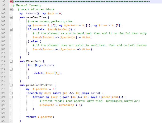
88 CONTINUED 88

89 CONTINUED 89

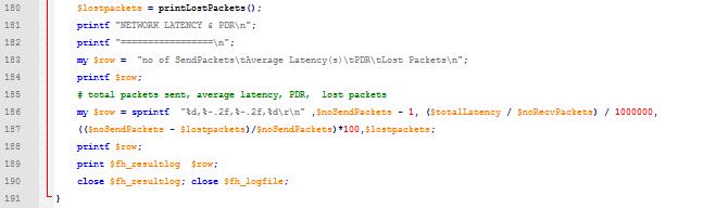
90 90