Formulas, LookUp Tables and PivotTables Prepared for Aero Controlex

Transcription

1 Basic Topics: Formulas, LookUp Tables and PivotTables Prepared for Aero Controlex Review ribbon terminology such as tabs, groups and commands Navigate a worksheet, workbook, and multiple workbooks Prepare data No blank rows or columns Format a header row (different format or capitalization) Remove pre-existing calculations Remove filters (look for funnel next to column name) Create a table Tables facilitate: Row and column formatting Removal of duplicates Automatic filter buttons Automatic functions in a total row Insert tab > Styles group > Format as Table Selection tips Group sheets Formulas Formulas are instructions to perform mathematical calculations on an Excel spreadsheet. Rules: All formulas begin with = Operators include + - * / Order of operations: Parentheses Exponentiation Multiplication and Division Addition and Subtraction Use the mouse or track pad to specify cells when writing a formula. Refer to cells and cell ranges in formulas Do not type specific numbers. Using cell addresses instead of specific numbers enables Excel to automatically calculate formula results when the data changes. Identify a range of cells by clicking the cell in the upper left corner (first cell in the range) followed by a colon (:) and then click the cell in the lower right corner (last cell in the range). An alternative is to drag the mouse pointer to select a range. Use Excel s fill handle to copy formulas down a column or across a row. The fill handle is a black that appears when you rest the mouse pointer in the lower right corner of a cell.

2 Functions Relative, Absolute and Mixed References When you copy a formula from one location to another, Excel adjusts the formula to its new location. This is called a relative reference. For example, if the cell address A1 is copied down a row, the row part of the formula will change to A2, A3, A4, etc. If the number in A1 is copied across a column to B1, the column part of the formula will change to B1, C1, D1, etc. To prevent a cell from adjusting the formula when copied, type $ before the cell address to be copied. This is called an absolute reference. For example, if the cell reference $C$1 is copied down or across, it will not change. A mixed reference includes both a relative and absolute reference. For example, if a formula in cell address C$1 is copied to cell D2, the reference to column C will change to D, but the reference to row 1 remains number 1. It is absolute. If a formula in cell $C1 is copied to cell D2, the reference to column C remains, but the reference to row 1 adjusts to row 2. Definition: A function is a built-in formula. Functions usually have a descriptive name, so it is easy to recognize what calculation the function will perform. Examples: SUM will add numbers in columns or rows. AVERAGE will average a range of numbers. MAX will find the highest number in a range. MIN will identify the lowest number in a range. More complex functions include VLOOKUP and IF. Functions are arranged in categories such as Financial, Logical and Lookup & Reference. Type a function or use the Function Wizard on the ribbon:

3 Errors If a formula or function contains an error, Excel displays an error message. Examples of error message include: Error Meaning #NULL! A space was used in formulas that reference multiple ranges; a comma separates range references #NUM! A formula has invalid numeric data for the type of operation #REF! A reference is invalid #VALUE! The wrong type of operand or function argument is used Tips Use descriptive range names for easy identification. Range names automatically create an absolute reference. Example: The range name Products could refer to cells B2:D51628 where Data in Column B = Product Name Data in Column C = Vendor Data in Column D = Price To create a range name: 1. Select the range you want to name. 2. Click in the Name box just above Column A. 3. Type a descriptive name that is not a cell address. (Example: Qtr1 is a cell address so it cannot be a range name.) 4. The first character in a range name must be a letter, not a number. 5. Do not use spaces in a range name. 6. Press Enter when you have finished.

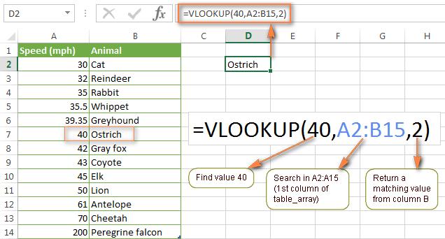
4 Excel VLOOKUP VLOOKUP is an Excel function used to look up data in a Vertical Column. The letter "V" in VLOOKUP stands for "vertical". It is used to differentiate VLOOKUP from the HLOOKUP function that looks up a value in the Top Row of an array (H stands for "horizontal"). VLookup is like looking up a phone number in a telephone book. (Remember those?) You tell Excel where the data is located (the phone book) and which data column the information you request (phone number) is located. Except instead of specifying the data itself, you specify the number of the column where the phone number resides, counting from the left side of the data. Another example is looking up a part number in a list of airplane parts. The syntax is: =VLOOKUP(lookupvalue,search_location,column#where_searched_item_is_located) Commas separate the 3 required components of a lookup function: Part 1 Part 2 Part 3 Part 4 One cell in a major list that contains data to look for A separate range where the data you seek is located A column number, counting from the left-most column, containing the data you need This data will be copied to the cell in the major list (Optional) TRUE or FALSE

5

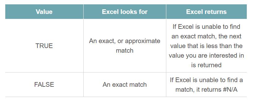
6 Rules: There are no spaces in the function. The lookup value MUST be located in the first column. The data reference must be an absolute reference to prevent it from changing when copying your VLookup formula to other cells. (Use $ before the column letter and $ before the row number). Example: $A1:$E5692 Excel will return an approximate value if you choose TRUE and the exact value is not within the range you specify. Use quotation marks ( ) to indicate you are searching for text ( Product 1 ) In VLOOKUP formulas, all values are case-insensitive, meaning that uppercase and lowercase characters are treated as equivalent. If the lookup value is smaller than the smallest value in the first column of table_array, the VLOOKUP function returns the #N/A error. If the 3rd parameter (col_index_num) is less than 1, the VLOOKUP formula will return the #VALUE! error. In case it is greater than the number of columns in table_array, the formula will return the #REF! error. When searching with approximate match (range_lookup set to TRUE or omitted), always have the data in the first column of table_array sorted in ascending order. And finally, remember about the importance of the last parameter. Supply TRUE for approximate match or FALSE for exact match, and it will save you a lot of headache. Good news! If the lookup range is in a different worksheet or even a different workbook, you don't have to type the name of the worksheet or workbook manually. Be sure the workbook file is open. Then simply start typing the formula. When it comes to the table_array argument, switch to the lookup worksheet or workbook and select the range using a mouse. Once you close the workbook with your lookup table, your VLOOKUP formula will work anyway, but it will display the full path for the lookup workbook, as shown below.

7 Using wildcard characters in VLOOKUP formulas As in many other formulas, you can use the following wildcard characters in the Excel VLOOKUP function: Question mark (?) to match any single character, and Asterisk (*) to match any sequence of characters. Using wildcard characters in your VLOOKUP formulas may prove useful in many cases: When you do not remember the exact text you are looking for. When you want to find some word that is part of the cell's contents. Be aware that the VLOOKUP function searches by the entire content of a cell, as if you selected the option "Match entire cell content" in the standard Excel Find dialog. When a lookup column contains extra leading or trailing spaces. (If that is the case, you may be puzzled trying to figure out why the normal formula does not work.) Example: Look up text starting or ending with certain characters Suppose you want to find a certain customer in the database below. You cannot remember his last name, but you know it starts with ack. So the following VLOOKUP formula will find what you need. =VLOOKUP("ack*",$A$2:$C$11,1,FALSE)

8 How to use a named range or table in VLOOKUP formulas If you use the same lookup range in several VLOOKUP formulas, you can created a named range for it and type the name directly in the table_array argument of your VLookup formula. To create a named range, just select the cells and type any name in the Name box, to the left of the Formula bar. And now you can write the following VLOOKUP formula to get Product 1's price: =VLOOKUP("Product 1",Products,2) Most range names in Excel apply to the entire workbook, so you don't need to specify the worksheet's name, even if your lookup range resides in a different worksheet. If it is in another workbook, you have to put the workbook's name before the named range, for example: =VLOOKUP("Product 1",PriceList.xlsx!Products,2) Using named ranges can be a good alternative to absolute cell references. Since a named range doesn't change when a formula is copied to other cells, you can be sure that your lookup range will always remain correct.

9 If you have converted a range of cells into a fully-functional Excel table (Insert tab > Table), then you can select the lookup range using a mouse, and Microsoft Excel will automatically add the columns' names or the table name to the formula. The complete formula may look similar to this: =VLOOKUP("Product 1",Table46[[Product]:[Price]],2) or even =VLOOKUP("Product 1",Table46,2). As well as named ranges, columns names are constant and your cell references won't change no matter where the VLOOKUP formula is copied within the same workbook. Using wildcard characters in VLOOKUP formulas As well as in many other formulas, you can use the following wildcard characters in the Excel VLOOKUP function: Question mark (?) to match any single character, and Asterisk (*) to match any sequence of characters. Using wildcard chars in your VLOOKUP formulas may prove really useful in many cases: When you do not remember the exact text you are looking for. When you want to find some word that is part of the cell's contents. Be aware that the VLOOKUP function searches by the entire content of a cell, as if you selected the option "Match entire cell content" in the standard Excel Find dialog. When a lookup column contains extra leading or trailing spaces. If it is the case, you may rack your brain trying to figure out why the normal formula does not work. Suppose, you want to find a certain customer in the below database. You cannot remember his surname, but you know it starts with "ack". So, the following VLOOKUP formula will work a treat: =VLOOKUP("ack*",$A$2:$C$11,1,FALSE)

10 Once you are sure you've found the correct name, you can use a similar VLOOKUP formula to get the sum paid by that customer. You only have to change the 3 rd parameter in the formula to the appropriate column number, column C (3) in our case: =VLOOKUP("ack*",$A$2:$C$11,3,FALSE) Here a few more examples of VLOOKUP formulas with wildcard characters: =VLOOKUP("*man",$A$2:$C$11,1,FALSE) - find the name ending with "man". =VLOOKUP("ad*son",$A$2:$C$11,1,FALSE) - find the name starting with "ad" and ending with "son". =VLOOKUP("?????",$A$2:$C$11,1,FALSE) - find a 5-character last name. Note. For a wildcard VLOOKUP formula to work correctly, you always have to add FALSE as the last parameter. If your lookup range contains more than one entry that meets the wildcard criteria, the first found value will be returned.

11 PivotTables What is a pivot table in Excel? An Excel pivot table, aka PivotTable, is a tool to explore and summarize large amounts of data, analyze related totals and present summary reports. Pivot table reports are essentially designed to: Present large amounts of data in a user-friendly way. Summarize data by categories and subcategories. Filter, group, sort and conditionally format different subsets of data so that you can focus on the most relevant information. Rotate rows to columns or columns to rows (which is called "pivoting") to view different summaries of the source data. Subtotal and aggregate numeric data in the spreadsheet. Expand or collapse the levels of data and drill down to see the details behind any total. Present concise and attractive online of your Excel data or printed reports. For example, you may have hundreds of entries in your Excel worksheet with sales figures of local resellers:

12 How to make a pivot table in Excel: quick start 1. Organize your source data in an Excel Table Before creating a pivot table, organize your data into rows and columns, and then convert your data range into an Excel Table. To do this, select all of the data, go to the Insert tab and click Table. Useful tips: Add unique, meaningful headings to your columns, they will turn into the pivot table's field names later. Make sure your source table contains no blank rows or columns, and no subtotals. To make it easier to maintain your pivot table, you can name your source table by switching to the Design tab and typing the name in the Table Name box the upper right corner of your worksheet. 2. Create a pivot table Select any cell in the source data table (if you are building a pivot table based on a range of cells, select all cells with the data that you want to include), and then go to the Insert tab > Tables group > PivotTable. This will open the Create PivotTable window. Make sure the correct table or range of cells is highlighted in the Table/Range field. Then choose the target location for your Excel pivot table: Selecting New Worksheet will place a pivot table in a new worksheet starting at cell A1. Selecting Existing Worksheet will place your pivot table at the specified location in an existing worksheet. In the Location box, click the Collapse Dialog button to choose the first cell where you want to position your pivot table. Clicking OK creates a blank pivot table in the target location. This will be the location of your new PivotTable. 3. Arrange the layout of your pivot table report The area where you work with the fields of your pivot tables is called PivotTable Field List. It is located in the right-hand part of the worksheet and divided into the header and body sections:

13 The Field Section contains the names of the fields that you can add to your pivot table. The filed names correspond to the column names of your source table. The Layout Section contains the Report Filter area, Column Labels, Row Labels area, and the Values area. Here you can arrange and re-arrange the fields of your pivot table. The changes that you make in the PivotTable Field List are immediately reflected to your pivot table. To add a field to the Layout section, select the check box next to the field name in the Field section. By default, Microsoft Excel adds the fields to the Layout section in the following way: Non-numeric fields are added to the Row Labels area Numeric fields are added to the Values area To delete a certain field from your Excel pivot table, you can either: Uncheck the box nest to the field's name in the Field section of the PivotTable pane. Right-click on the field in your pivot table, and then click "Remove Field_Name". To arrange pivot table fields: 1. Drag and drop fields between the 4 areas of the Layout section using the mouse. Alternatively, click and hold the field name in the Field section, and then drag it to an area in the Layout section - this will remove the field from the current area in the Layout section and place it in the new area. 2. Right-click the field name in the Field section, and then select the area where you want to add it. 3. Click on the filed in the Layout section to select it. This will also display the options available for that particular field.

14 4. Choose the function for the Values field (optional) By default, Microsoft Excel uses the Sum function for numeric value fields that you place in the Values area of the PivotTable Field List. When you place non-numeric data (text, date, or Boolean) or blank values in the Values area, the Count function is applied. The Summarize Values By option is available on the ribbon - on the Options tab, in the Calculations group. The functions' names are mostly self-explanatory: Sum - calculates the sum of the values. Count - counts the number of non-empty values (works as the COUNTA function). Average - calculates the average of the values. Max - finds the largest value. Min - finds the smallest value. Product - calculates the product of the values. Tips: Drag and drop fields to see how the power of a PivotTable can be easily manipulated. Right-click a cell for additional actions. Double-click any cell to "drill down" that data, which will create a new worksheet and show all records from the data source which went into that value. Group fields in an existing PivotTable o Right-click or choose Group from ribbon 5. Show different calculations in Pivot Table value fields (optional) Excel pivot tables provide one more useful feature that enables you to present values in different ways, for example show totals as percentage or rank values from smallest to largest and vice versa. The full list of calculation options is available here.

15 This feature is called Show Values As and it's accessible by right-clicking the field in the table in Excel 2016 and In Excel 2010 and lower, you can also find this option on the Options tab, in the Calculations group. Tip. The Show Values As feature may prove especially useful if you add the same field to a pivot table more than once and show, for example, total sales and sales as a percent of total at the same time.

16 Working with PivotTable Field List The pivot table pane, which is formally called PivotTable Field List, is the main tool that you use to arrange your summary table exactly the way you want. To make your work with the fields more comfortable, you may want to customize the pane to your liking. Changing the Field List view How to use pivot table in Excel Now that you know the pivot table basics, you can navigate to the Analyze and Design tabs of the PivotTable Tools in Excel 2016 and 2013 (Options and Design tabs in Excel 2010 and 2007) to explore the groups and options provided there. These tabs become available as soon as you click anywhere within your pivot table. You can also access options and features that are available for a specific pivot table element by right-clicking that element. How to get rid of "Row Labels" and "Column Labels" headings When you are creating a pivot table, Excel applies the Compact layout by default. This layout displays "Row Labels" and "Column Labels" as headings in the pivot table. These aren't very meaningful headings. An easy way to get rid of these headings is to switch the pivot table layout from Compact to Outline or Tabular. To do this, go to the Design ribbon tab, click the Report Layout dropdown, and choose Show in Outline Form or Show in Tabular Form.

17 This will cause your Excel pivot table to display the actual field names, as you see in the pivot table on the right, which makes much more sense. Another solution is to go to the Analyze (Options) tab, click the Options button, switch to the Display tab and uncheck the "Display Field Captions and Filter Dropdowns" box. However, this will remove all field captions as well as filter dropdowns in your pivot table. How to insert a slicer in a pivot table A slicer is similar to a filter, except choices are displayed in a dialog box. Click on any cell within the PivotTable for which you want to create a slicer. This activates a PivotTable contextual tab. On the Options tab, in the Sort & Filter group, click on the Insert Slicer button. In the Insert Slicers dialog box, click the checkboxes by the PivotTable fields you want to filter by. Note: You may need to hold the CTRL key to select multiple checkboxes. A slicer will be created on the same worksheet for every field that you select. Data in fields that are checked are displayed. Data in unchecked fields are hidden. How to insert a timeline in a pivot table A timeline is similar to a date filter, except choices are displayed in a dialog box. Click on any cell within the PivotTable for which you want to create a timeline. This activates a PivotTable contextual tab. On the Options tab, In the Sort & Filter group, click on the Insert Timeline button. In the Insert Timeline dialog box, click the checkboxes by the PivotTable dates you want to filter. Note: You may need to hold the CTRL key to select multiple checkboxes. A timeline will be created on the same worksheet for every field that you select. Dates in fields that are checked are displayed. Dates in unchecked fields are hidden.

18 How to refresh a pivot table in Excel Although a pivot table report is connected to your source data, you might be surprised to know that Excel does not refresh it automatically. You can get any data updates by performing a refresh operation manually, or have it refresh automatically when you open the workbook. Refresh the pivot table data manually 1. Click anywhere in your pivot table. 2. Right-click the pivot table, and choose Refresh from the context menu. To refresh all pivot tables in your Excel workbook, click the Refresh button arrow, and then click Refresh All. Note. If the format of your pivot table gets changed after refreshing, make sure the "Autofit column width on update" and "Preserve cell formatting on update" options are selected. After starting a refresh, you can review the status or cancel it if you've changed your mind. Just click on the Refresh button arrow, and then click either Refresh Status or Cancel Refresh. Refreshing a pivot table automatically when opening the workbook 1. On the Analyze / Options tab, in the PivotTable group, click Options > Options. 2. In the PivotTable Options dialog box, go to the Data tab, and select the Refresh data when opening the file check box.

19 How to delete an Excel pivot table If you no longer need a certain pivot table, you can delete it in a number of ways. If your pivot table resides in a separate worksheet, simply delete that sheet. If your pivot table is located along with some other data on a sheet, select the entire pivot table using the mouse and press the Delete key. Click anywhere in the pivot table that you want to delete, go to the Analyze tab in Excel 2016 and 2013 (Options tab in Excel 2010 and earlier) > Actions group, click the little arrow below the Select button, choose Entire PivotTable, and then press Delete. Pivot table examples The screenshots below demonstrate a few possible pivot table layouts for the same source data that might help you to get started on the right path. Pivot table example 1: Two-dimensional table

20 No Filter Rows: Product, Reseller Columns: Months Values: Sales

21 Pivot table example 2: Three-dimensional table Filter: Month Rows: Reseller Columns: Product Values: Sales This pivot table lets you filter the report by month.

22 Pivot table example 3: One field is displayed twice - as total and % of total No Filter Rows: Product, Reseller Values: SUM of Sales, % of Sales This pivot table shows total sales and sales as a percent of total at the same time.