INTRODUCTION TO EXCEL 2010

Transcription

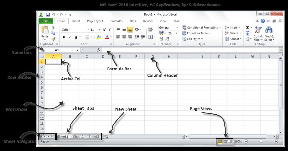
1 INTRODUCTION TO EXCEL 2010 Microsoft Excel is a spreadsheet program that's designed to record and analyze numbers and data. Excel takes the place of a calculator, a ruled ledger pad, pencils and pens, etc. The program makes it easy for you to manage numbers, formulas, and text. Workbook: An Excel file is called a workbook. Each workbook consists of several worksheets made up of rows and columns of information. By default there will be 3 worksheets. You can add up to a maximum of 255 worksheets in a workbook. Worksheet: One sheet in an Excel workbook. Each worksheet consists of columns and rows. Total characters inside a single cell can be up to The worksheets are numbered automatically from Sheet 1 to Sheet 256. Cell: Where a row and column intersect, each cell has an address that consists of the column letter and row number (A1, B3, C4, and so on). You enter data and formulas in the cells to create your worksheets. STARTING EXCEL: Click Start. Click All Programs. Click Microsoft Office. Click Microsoft Excel EXCEL INTERFACE COMPONENTS The Name box displays the active cell address. The formula bar allows you to enter or edit data in the worksheet. The cell pointer is a dark rectangle that outlines the cell you are working in. This cell is called the active cell. Sheet tabs below the worksheet grid let you switch from sheet to sheet in a workbook. By default, a workbook file contains three worksheets but you can use just one, or have as many as 255, in a workbook. The Insert Worksheet button to the right of Sheet 3 allows you to add worksheets to a workbook. Sheet tab scrolling buttons let you navigate to additional sheet tabs when available. You can use the scroll bars to move around in a worksheet that is too large to fit on the screen at once. The status bar is located at the bottom of the Excel window. It provides a brief description of the active command or task in progress. The mode indicator in the lower-left corner of the status bar provides additional information about certain tasks.

2

3 COMMON MOUSE POINTERS IN EXCEL: Pointer Action Moves the cell pointer or to select range of the cells Adjusts the row height Adjusts the column width Moves the insertion point within the cell Moves the cell from one place to another AutoFills other cells with similar data Selects the entire row Selects the entire column STARTING A NEW WORKBOOK: Click on File Or Click on icon on the Quick Access toolbar Or Press Ctrl + N on the keyboard Chose New From the Available Templates category choose Blank workbook Click Create button SAVING A WORKBOOK: Click File Save Or click the Save button on the Quick Access toolbar or press Ctrl+S. The Save As dialog box appears.

4 Type the name you want to give the workbook in the File Name text box. You can use up to 218 characters, including any combination of letters, numbers, and spaces. Normally, Excel saves your workbooks in the Documents folder. To save the file to a different folder or drive, select a new location. Click Save or press Enter to save your workbook. Note: To save changes that you make to a workbook that you have previously saved, just click the Save button on the Standard toolbar. You can also press the shortcut key combination of Ctrl+S to save changes to your workbook. SAVING A WORKBOOK UNDER A NEW NAME OR LOCATION: Click File Save As. The Save As dialog box opens. Type the new filename in the File Name text box. Select the drive letter or the folder. Click the Save button or press Enter. OPENING AN EXISTING WORKBOOK: Click File Open, or click the Open button on the Quick Access toolbar or press Ctrl+O on the keyboard. The Open dialog box appears. If the file is not located in the current folder, select the correct drive and folder. Select the file you want to open in the files and folders list. Click Open to open the currently selected workbook. CLOSING WORKBOOKS AND APPLICATION: When you have finished with a particular workbook and want to continue working in Excel, you can easily close the current workbook. Click the Close (X) button in the upper-right corner of the workbook.

5 You can also close the current workbook by selecting File Close. If you have changed the workbook since the last time you saved it, you will be prompted to save any changes. If you want click Yes button or click No to discard changes. Or click Cancel to remain with the workbook. When you have finished working with Excel application itself, you can close the entire program itself by choosing File Exit option MOVING WITHIN EXCEL: Keys Press Enter Shift+Enter Tab Shift+Tab Up, Down, Right, Left Arrow keys Ctrl+Right Arrow or Ctrl+Left Arrow Ctrl+Up Arrow or Ctrl+Down Arrow Home Ctrl+Home Page Up Page Down Ctrl+ Page Up Ctrl + Page Down Alt + Page Up Alt + Page Down F5 Moves To One cell down or to the next cell in sequence One cell up One cell to the right One cell to the left One cell in the direction of the arrow To the right or left end of a row that contains data (if there is no data the cell goes to the end or beginning of the worksheet right side or left side) To the top or bottom of a column that contains data (if there is no data the cell goes to the end or beginning of the worksheet top or bottom) To the first cell in the row To the first cell in the worksheet Up one screen Down one screen Moves to next worksheet Moves to previous worksheet One screen to the right One screen to the left Display the Go to Dialog Box ENTERING TEXT, NUMBERS AND DATES & TIMES: Text is any combination of letters, numbers, and spaces. By default, text is automatically left-aligned in a cell, whereas numerical data is right-aligned. To enter text into a cell, follow these steps: o Use your mouse or the keyboard arrows to select the cell in which you want to enter text, Type the text. o As you type, your text appears in the cell and in the Formula bar, Press Enter. o Your text appears in the cell, left-aligned. o The cell selector moves down one cell. You can also press Tab or an arrow key to enter the text and move to the next cell to the right (or in the direction of the arrow). (If you want to enter multiple lines within a cell press and hold the Alt key and press Enter key to create new line).

6 Exercise 01: enter the following data in Excel and save your workbook as MyNameList.xlsx To enter number into a cell, follow these steps: o Click in the cell where you want to enter the value, Type the value. o To enter a negative number, precede it with a minus sign or surround it with parentheses. o Press Enter or the Tab key; the value appears in the cell right-aligned. Exercise 02: open the workbook MyNameList.xlsx and modify it as follows To enter date or time, follow these steps: o Click in the cell where you want to enter a date or a time, to enter a date o Use the format MM/DD/YY or the format MM-DD-YY, as in 5/9/03 or (Depends on your computer s setting). o To enter a time, be sure to specify a.m. or p.m., as in 7:21 p or 8:22 a. o Press Enter. As long as Excel recognizes the entry as a date or a time, it appears right-aligned in the cell. o If Excel doesn't recognize it, it's treated as text and left-aligned. (Note that the format can vary according to the Date and Time setting of your system) Exercise 03: open the workbook MyNameList.xlsx and modify it as follows Note: To enter current date press Ctrl + ; on the keyboard.

7 To enter current time press Ctrl + Shift + : on the keyboard EDITING INFORMATION: To overwrite the existing contents of a cell, click on the cell you want to change and type the new contents. If you want to change part of the contents, double click or press F2 key to bring the cell in edit mode. An insertion point will appear in the cell. You can then enter the changes or delete the text or numbers as required (you can do it directly in Formula Bar itself). COPYING DATA: When you copy data, you create a duplicate of data in a cell or range of cells. Follow these steps to copy data: Select the cell(s) that you want to copy. You can select any range or several ranges if you want. Click the copy button on the Clipboard group in the Home ribbon or press Ctrl+C Select the first cell in the area where you would like to place the copy. Click the paste button on the Clipboard group in the Home ribbon or press Ctrl+V. MOVING DATA: To move data, follow these steps: Select the cells you want to move. Click the cut button on the Clipboard group in the Home ribbon or press Ctrl+X. Select the first cell in the area where you want to place the data. Click paste on the Clipboard group in the Home ribbon or press Ctrl+V. DELETING DATA: To delete the data in a cell or range of cells, select them and press Delete. Or select Clear All from the Clear button of the Editing group in the Home ribbon. USING FILL FEATURE: Click the fill handle of the cell (the small block in the lower-right corner of the cell) that holds the data that you want to copy. Drag the fill handle down or to the right to copy the data to adjacent cells. Release the mouse button. The data is "filled" into the selected cells. Note: If you want to create a series such as 10, 20, 30, where the series uses a custom increment between the values, you need to create a custom series. Excel provides two ways to create a custom series. To create a custom series using Fill, follow these steps: o o o Enter the first value of the series into a cell. Enter the second value in the series into the next cell. This lets Excel know that the increment for the series. Select both cells by clicking the first cell and dragging over the second cell.

8 o Drag the fill handle of the second cell to the other cells that will be part of the series. Excel analyzes the two cells, sees the incremental pattern, and re-creates it in subsequent cells. Exercise 04: Create the following in a worksheet and save it as AutoFillExercise.xlsx USING THE REPLACE FEATURE: Suppose you've entered a particular label or value into the worksheet and find that you have consistently entered it incorrectly. A great way to change multiple occurrences of a label or value is using Excel's Replace feature; you can locate data in the worksheet and replace it with new data. To find and replace data, follow these steps: Select the Find & Select button to invoke its dropdown list and choose Replace or press Ctrl + H. The Find and Replace dialog box appears. Type the text or value that you want to find into the Find What text box. Click in the Replace With text box and type the text you want to use as replacement text and click Find Next button to find the first occurrence of your specified entry. If Excel locates, click on Replace button to replace the particular item or click Replace All to replace all matching items. Once the process is over, click Close button.

9 ENTER DATA INTO A CELL Click the cell in which you want to enter the data. Start typing your data. When your data entry is complete, press Enter. EDIT CELL DATA Click the cell in which you want to edit the data and press F2 key or double click on the cell Make your changes to the cell data. When you finish editing the data, press Enter key DELETE DATA FROM A CELL Select the cell that contains the data you want to delete. Click the Home tab. Click Clear Click Clear Contents. UNDO CHANGES Click the Undo button. Excel reverses the effects of the last change you made. You can repeatedly click to reverse each action you have taken, from last to first. You can also press Ctrl + Z to reverse an action. If you decide not to reverse an action after clicking Undo button, click the Redo button.

10 FORMATTING TEXT AND NUMBERS When you work in Excel, you work with two types of formatting: value formatting and font formatting. In value formatting, you assign a particular number style to a cell (or cells) that holds numeric data. You can assign a currency style, a percent style, etc. Another formatting option available to you in Excel relates to different font attributes. USING THE STYLE BUTTONS TO FORMAT NUMBERS: The Formatting toolbar contains several buttons for applying a format to your numbers. To use one of these buttons, select the cell or cells you want to format, and then click the desired button. CHANGING TEXT ATTRIBUTES WITH FONT GROUP To use the Formatting toolbar to change text attributes, follow these steps: Select the cell or range that contains the text whose look you want to change. To change the font, click the Font drop-down list, and select a new font name. To change the font size, click the Font Size drop-down list and select the size you want to use. You can also type the point size into the Font Size box and then press Enter. To add an attribute such as bold, italic, or underlining to the selected cells, click the appropriate button: Bold, Italic, or Underline, respectively. You can also change the color of the font in a cell or cells. Select the cell or cells and click the Font Color dropdown arrow on the Formatting toolbar. Select a font color from the Color palette that appears. NUMERIC FORMATTING OPTIONS: Excel's Format Cells dialog box offers a wide range of number formats and even allows you to create custom formats. To use the Format Cells dialog box to assign numeric formatting to cells in a worksheet, follow these steps: Select the cell or range that contains the values you want to format. Select Format Cells. The Format Cells dialog box appears. Click the Number tab. The different categories of numeric formats are displayed in a Category list. In the Category list, select the numeric format category you want to use. The sample box displays the default format for that category. Click OK to assign the numeric format to the selected cells.

11 ACCESSING DIFFERENT FONT ATTRIBUTES: If you would like to access a greater number of font format options for a cell or range of cells, you can use the Font tab of the Format Cells dialog box. Follow these steps: Select the cell or range that contains the text you want to format. Right click and choose Format Cells, or press Ctrl+1. Click the Font tab. The Font tab provides drop-down lists and check boxes for selecting the various fonts attributes. Select the options you want. Click OK to close the dialog box and return to your worksheet. ALIGNING TEXT IN CELLS: Both text and numbers are initially set at the bottom of the cells. However, you can change both the vertical and the horizontal alignment of data in your cells. Follow these steps to change the alignment: Select the cell or range you want to align. Select Format Cells. The Format Cells dialog box appears. Click the Alignment tab. Choose from the options such as Text alignment, Orientation etc. to set the alignment Click OK when you have finished making your selections.

12 COMBINING CELLS AND WRAPPING TEXT: Combining a group of cells also allows you to place a special heading or other text into the cells. Select the cells that you want to combine. Invoke the Format Cells dialog box by pressing Ctrl+1. Click the Merge Cells check box and then click OK. The cells are then merged. You might want to wrap the text within the cell or merged cells. Select the cells that you want to combine. Invoke the Format Cells dialog box by pressing Ctrl+1. Click the Wrap Text checkbox. Then click OK. ADDING BORDERS TO CELLS: To create well-defined lines on the printout (or onscreen), you can add borders to selected cells or entire cell ranges. A border can appear on all four sides of a cell or only on selected sides; it's up to you. To add borders to a cell or range, perform the following steps: Select the cells that you want to combine. Invoke the Format Cells dialog box by pressing Ctrl+1. Click the Border tab to see the Border options. Select the borders, lines styles, color, etc. Click OK or press Enter.

13 Note: You can use the Borders button on the Formatting toolbar to add a border to cells or cell ranges. Select the cells, and then click the Borders drop-down arrow on the Formatting toolbar to select a border type. ADDING SHADING TO CELLS: With shading, you can add a color or gray shading to the background of a cell. You can add shading that consists of a solid color, or you can select a pattern as part of the shading options, such as a repeating diagonal line. Follow these steps to add shading to a cell or range. Select the cell(s) you want to shade. Choose Format Cells. Click the Patterns tab. Excel displays the shading options. Click the Pattern drop-down arrow to see a grid that contains colors and patterns.

14 Select the shading color and pattern you want to use. A preview of the results appears in the Sample box. When you have finished making your selections, click OK. Note: You can also use Fill Color button on the Formatting toolbar. Select the cells you want to shade. Click the Fill Color drop-down arrow on the Formatting toolbar and then select the fill color from the Color palette that appears. Exercise 05 - PC Application by S. Sabraz Nawaz 2012 Quarterly Budget Projection Quarter 1 Quarter 2 Quarter 3 Quarter 4 Total Income Sales Cost of Goods Sold Gross Margin Expenses Overhead Marketing Salaries Legal Fees Total Expenses Profit Hint: Merge the Heading cells Use Fill handle to enter Quarters Use SUM function to find totals Apply the formatting as shown Gross Margin = Sales - Cost of Goods Sold Total Expenses = Overhead + Marketing + Salaries + Legal Fees Profit = Gross Margin - Total Expenses Exercise 06 - PC Application by S. Sabraz Nawaz Production Plan for PCApplication Company Sales Volume Selling Price per Unit Material Price per Unit Labour Cost (% of Sales Revenue) 16% 16% 18% 18% Factory Overheads

15 Sales Revenue Material Cost Labour Costs Prime Cost Contributions Gross Profit / Loss Profit Percentage (%) Hints: Sales Revenue = Sales Volume * Selling Price per unit Material Cost = Sales Volum * Material Price Labour Cost = Sales Revenue * Labour Cost Prime Cost = Material Cost + Labour Cost Contribution = Sales Revenue - Prime Cost Gross Profit = Contribution - Factory Overhead Profit Percentage = Gross Profit / Sales Apply proper formatting Merge the Heading cells Exercise 07 - PC Application by S. Sabraz Nawaz Cash Book of MIT Company (Pvt) Ltd. Date 1-Jan-12 1-Feb-12 1-Mar-12 1-Apr-12 (In Rs 000) (In Rs 000) (In Rs 000) (In Rs 000) Balance B/F Receipts Cash Sales From Debtors Loan Recovery Total Receipts Payments Cash Purchase To Creditors Expenses Loan Payments Total Payments Cash In Hand Hint:

16 Balance B/F is the Cash in Hand of the previous month Apply the formatting Exercise 08 - PC Application by S. Sabraz Nawaz Salary Schedule of MIT PC Application (Pvt) Ltd for 2012 EPF - Employee 8% EPF - Company 12% ETF 3% Name Sabraz Dhammika Sampath Abee Kavindree Rashida Rizvi Sex M M M F F F M Department MIS MIS Finance Finance Marketing Marketing Finance Emp. No Emp 129 Emp 130 Emp 131 Emp 132 Emp 133 Emp 134 Emp 135 Date Joined 1/1/2006 1/1/2000 1/1/2011 1/1/2009 1/1/2010 1/1/2010 1/1/2006 Basic Salary Allowance (10%) Gross Salary Loan EPF - Employee Total Deduction Net Salary EPF - Company ETF Total Salary Hints: Allowance is 10% of the Basic Salary EPFs and ETF are calculated from Basic Salary Apply the formatting shown APPLYING CONDITIONAL FORMATTING:

17 Another useful formatting feature that Excel provides is conditional formatting. Conditional formatting allows you to specify that certain results in the worksheet be formatted so that they stand out from the other entries in the worksheet. To apply conditional formatting, follow these steps: Select the cells to which you want to apply the conditional formatting. Select Format Conditional Formatting. The Conditional Formatting dialog box appears. Be sure that Cell Value Is is selected in the Condition 1 drop-down box on the left of the dialog box. In the next drop-down box to the right, select the condition. Click the Collapse button to specify a cell or cells in the worksheet that Excel can use as a reference for the conditional formatting. Click the Expand button on the Conditional Formatting dialog box to expand the dialog box. Click the Format button in the Conditional Formatting dialog box and select the formatting options for your condition in the Format Cells dialog box. Then click OK. After setting the conditions to be met for conditional formatting (you can click Add to set more than one condition), click OK. INSERTING ROWS AND COLUMNS: Inserting entire rows and columns into your worksheet is very straightforward. Follow these steps: To insert a single row or column, select a cell to the right of where you want to insert a column or below where you want to insert a row (to insert multiple columns or rows, select the number of columns or rows you want to insert).

18 Select Insert Rows or Insert Columns. Excel inserts rows above your selection or columns to the left of your selection. Note: to quickly insert rows or columns, select one or more rows or columns, right-click one of them, and choose Insert from the shortcut menu. FREEZING COLUMN AND ROW LABELS: When you work with very large worksheets, it can be very annoying as you scroll to the right or down through the worksheet and you can no longer see your row headings or column headings, respectively. You can freeze your column and row labels so that you can view them no matter how far you scroll down or to the right in your worksheet. To freeze row or column headings (or both), follow these steps: Click the cell to the right of the row labels and/or below any column labels you want to freeze. This highlights the cell. Select the Window Freeze Panes. Note: To unfreeze them, select Window Unfreeze Panes. HIDING COLUMNS, ROWS AND WORKSHEETS: To hide a row or a column in a worksheet, click a row or a column heading to select it. Then, right-click within the row or column and select Hide from the shortcut menu that appears. The row or column will be hidden. To unhide the row or column, right-click the border between the hidden rows or columns that are visible, and then select Unhide from the shortcut menu. To hide a worksheet, click its tab to select it. Then, choose Format Sheet Hide. To unhide the worksheet, choose Format Sheet Unhide. Select the worksheet to unhide in the Unhide dialog box that appears, and then click OK. LOCKING CELLS IN A WORKSHEET: Locking cells in a worksheet is a two-step process. You must first select and lock the cells. Then, you must turn on protection on the entire worksheet for the "lock" to go into effect. Follow these steps to lock cells on a worksheet:

19 Select the cells in the worksheet that you want to lock. Select Format Cells. The Format Cells dialog box appears. Click the Protection tab. Be sure the Locked check box is selected on the Protection tab. Then click OK. Now select the Tools Protections Protect Sheet. The Protect Sheet dialog box appears. Enter a password if you want to require a password for "unprotecting" the worksheet. Then click OK. REMOVING ROWS AND COLUMNS: When you delete a row in your worksheet, the rows below the deleted row move up to fill the space. When you delete a column, the columns to the right shift left. Follow these steps to delete a row or column: Click the row number or column letter of the row or column you want to delete. You can select more than one row or column by dragging over the row numbers or column letters. Select Edit Delete. Excel deletes the rows or columns and renumbers the remaining rows and columns sequentially. All cell references in formulas and functions are updated appropriately.

20 INSERTING CELLS: Inserting cells causes the data in existing cells to shift down a row or over a column to create a space for the new cells. To insert a single cell or a group of cells, follow these steps: Select the area where you want the new cells inserted. Excel inserts the same number of cells as you select. Select Insert Cells. The Insert dialog box appears. Select Shift Cells Right or Shift Cells Down (or you can choose to have an entire row or column inserted). Click OK. Excel inserts the cells and shifts the adjacent cells in the direction you specify. REMOVING CELLS: Eliminating cells from the worksheet rather than just clearing their contents means that the cells surrounding the deleted cells in the worksheet are moved to fill the gap that is created. Remove cells only if you want the other cells in the worksheet to shift to new positions. Otherwise, just delete the data in the cells or type new data into the cells. If you want to remove cells from a worksheet, use the following steps: Select the cell or range of cells you want to remove. Choose Edit Delete. The Delete dialog box appears. Select Shift Cells Left or Shift Cells Up to specify how the remaining cells in the worksheet should move to fill the gap left by the deleted cells. Click OK. Surrounding cells are shifted to fill the gap left by the deleted cells. ADJUSTING COLUMN WIDTH AND ROW HEIGHT WITH A MOUSE: To adjust a column width with the mouse, place the mouse pointer on the right border of the column. A sizing tool appears. Drag the column border to the desired width. You can also adjust the column width to

21 automatically accommodate the widest entry within a column; just double-click the sizing tool. This is called AutoFit, and the column adjusts according to the widest entry. If you want to adjust several columns at once, select the columns. Place the mouse on any of the column borders and drag to increase or decrease the width. Each selected column is adjusted to the width you select. Changing row heights is similar to adjusting column widths. Place the mouse on the lower border of a row and drag the sizing tool to increase or decrease the row height. To change the height of multiple rows, select the rows and then drag the border of any of the selected rows to the desired height. USING THE FORMAT MENU FOR ADJUSTING COLUMN WIDTH AND ROW HEIGHT: If you want to precisely specify the width of a column or columns or the height of a row or rows, you can enter specific sizes using a dialog box. To specify a column width, follow these steps: Select the columns you want to change. Select Format Column Width. The Column Width dialog box appears. Type the column width into the dialog box. Click OK. Your column(s) width is adjusted accordingly. Adjusting row heights is similar to adjusting column widths. Select the row or rows, and then select the Format Rows Height. Row Height dialog box that appears. Type in the row height and then click OK. SELECTING WORKSHEETS: By default, each workbook consists of three worksheets whose names appear on tabs at the bottom of the Excel window. You can add or delete worksheets as desired. To select a worksheet or worksheets, perform one of the following actions: To select a single worksheet, click its tab. The tab becomes highlighted to show that the worksheet is selected.

22 To select several neighboring or adjacent worksheets, click the tab of the first worksheet in the group and then hold down the Shift key and click the tab of the last worksheet in the group. Each worksheet tab will be highlighted (but only the first sheet selected will be visible). To select several nonadjacent worksheets, hold down the Ctrl key and click each worksheet's tab. If you select two or more worksheets, they remain selected as a group until you ungroup them. To ungroup worksheets, do one of the following: Right-click one of the selected worksheets and choose Ungroup Sheets. Hold down the Shift key and click the tab of the active worksheet. (Ctrl key can also be used based on the preference) Click any worksheet tab to deselect all the other worksheets. INSERTING WORKSHEETS: When you create a new workbook, it contains three worksheets. You can easily add additional worksheets to a workbook. Follow these steps to add a worksheet to a workbook: Select the worksheet that you want to be to the right of the inserted worksheet. Select Insert Worksheet. Excel inserts the new worksheet to the right of the previously selected worksheet.

23 Note: A faster way to work with worksheets is to right-click the worksheet's tab. This brings up a shortcut menu that enables you to insert, delete, rename, move, copy, or select all worksheets. DELETING WORKSHEETS: If you find that you have a worksheet you no longer need, or if you plan to use only one worksheet, you can remove the unwanted worksheets. Here's how you remove a worksheet: Select the worksheet(s) you want to delete. Select Edit Delete Sheet. If the sheet contains data, a dialog box appears, asking you to confirm the deletion. Click Delete to delete the sheet. You will lose any data that the sheet contained. MOVING AND COPYING WORKSHEETS: You can move or copy worksheets within a workbook or from one workbook to another. Copying a worksheet enables you to copy the formatting of the sheet and other items, such as the column labels and the row labels. Follow these steps:

24 Select the worksheet(s) you want to move or copy. If you want to move or copy worksheets from one workbook to another, be sure the target workbook is open. Select Edit Move or Copy Sheet. The Move or Copy dialog box appears. To move the worksheets to a different workbook, be sure that workbook is open, and then select that workbook's name from the To Book drop-down list. If you want to move or copy the worksheets to a new workbook, select (New Book) in the To Book drop-down list. Excel creates a new workbook and then copies or moves the worksheets to it. In the Before Sheet list box, choose the worksheet you want to follow the selected worksheets. To move the selected worksheet, skip to next step. To copy the selected worksheets instead of moving them, select the Create a Copy option. Select OK. The selected worksheets are copied or moved as specified. Note: A fast way to copy or move worksheet(s) within a workbook is to use drag and drop. First, select the tab of the worksheet(s) you want to copy or move. Move the mouse pointer over one of the selected tabs, click and hold the mouse button, and drag the tab where you want it moved. To copy the worksheet, hold down the Ctrl key while dragging. When you release the mouse button, the worksheet is copied or moved. MOVING OR COPYING A WORKSHEET BETWEEN WORKBOOKS WITH DRAG AND DROP: You can also use the drag-and-drop feature to quickly copy or move worksheets between workbooks. Open the workbooks you want to use for the copy or move. Select Window Arrange. The Arrange dialog box opens. You can arrange the different workbook windows horizontally, vertically, tiled, or cascaded in the Excel application window. After making your selection, click OK to arrange the workbook windows within the Excel application window. Select the tab of the worksheet(s) you want to copy or move. Move the mouse pointer over one of the selected tabs, click and hold the mouse button, and drag the tab where you want it moved. To copy the worksheet, hold down the Ctrl key while dragging.

25 When you release the mouse button, the worksheet is copied or moved. CHANGING WORKSHEET NAMES By default, all worksheets are named Sheet1, Sheet2 So you should change the names that appear on the tabs that you'll have a better idea of the information each sheet contains,. Here's how to do it: Double-click the tab of the worksheet you want to rename. The current name is highlighted. Type a new name for the worksheet and press Enter. Excel replaces the default name with the name you type.

26 UNDERSTANDING EXCEL FORMULAS One way to add calculations to an Excel workbook is to create your own formulas. Formulas are typically used to perform calculations such as addition, subtraction, multiplication, and division. More complex calculations are better left to Excel functions, which is a built-in set of formulas that provide financial, mathematical, and statistical calculations. OPERATORS: You can create formulas that add, subtract, and multiply cells in the worksheet. The following are operators that you can use in a simple formula. Arithmetic Explanation Example + Addition Subtraction Negation -7 * Multiplication 7*3 / Division 7/2 % Percent 90% ^ Exponentiation 7^2 Comparison Explanation Example = Equal to B1=D1 > Greater than B1>D1 < Less than B1<D1 >= Greater than or equal to B1>=D1 <= Less than or equal to B1<=D1 <> Not equal to B1<>D1 Text Explanation Example & Adjoins text or cell references or any combination thereof "Sabraz" & " Nawaz" produces "SabrazNawaz" ORDER OF OPERATIONS / ORDER OF PRECEDENCE: The order of operations, or operator precedence, simply means that some operations take precedence over other operations in a formula. For example, to find the tax amount (figure shown) in the formula =C2-D2*E2, the multiplication of D2 times E2 takes precedence, so D2 is multiplied by E2 and then the resulting amount is subtracted from C2, this is not our purpose!! You can force the precedence of an operation by using parentheses. For example, if you want D2 subtracted from C2 before they are multiplied by E2, the formula would have to be written as =(C2- D2)*E2.

27 The natural order of precedence for math operators follows: Operators Process Parentheses All calculations within parentheses are completed first. Percent Percentages (for example, 12%) are calculated next, so that the actual value (in this case,.12) is used in the remaining calculations. Exponentiation Exponents (for example, 10^3, which means 10 cubed) are calculated next, so that the actual value is used in the remaining calculations. Multiplication Performed after parenthetical operations and before all other calculations. Division Follows any multiplication and is on the same level of precedence as multiplication. Addition Performed after all divisions. Subtraction Follows any additions and is on the same level of precedence as addition. ENTERING FORMULAS: Excel gives you two options for entering formulas: You can use the point-and-click technique or type the formulas. USING POINT-AND-CLICK ENTRY: Select the cell in which you want the formula's result to appear. Type the equal sign (=). Click the cell whose address you want to appear first in the formula. The cell address appears in the formula bar. Type an operator after the value to indicate the next operation you want to perform. For example, type + to add the next entry, to subtract, * to multiply, or / to divide by. Continue clicking cells and typing operators until you finish entering the formula. (Remember to group operations using parentheses, if necessary, to control the order of operations.) When you finish, press Enter to accept the formula. TYPING FORMULAS MANUALLY:

28 To type a formula, click the cell in which you want the formula's result to appear, and then type the formula, starting with an equal sign. To use a value from another cell in your formula, type the cell's address. EDITING FORMULAS: Editing a formula is same as editing any entry in Excel. The following steps show how you do it: Select the cell that contains the formula you want to edit. Click in the Formula bar to place the insertion point in the formula, or press F2 to enter Edit mode. Press the left-arrow key or the right-arrow key to move the insertion point within the formula. Then, use the Backspace key to delete characters to the left, or use the Delete key to delete characters to the right. Type any additional characters. When you finish editing, press Enter to accept your changes. COPYING AND PASTING FORMULAS: You can copy and paste formulas just as easily as you copy and paste data entries. When you paste a formula, however, Excel adjusts the cell references in the formula to reflect their new positions in the worksheet. Follow these steps to copy formulas Enter your formula in the first cell Select the cell containing the formula. The active cell (or range) has a small black box in the lower-right corner, called a fill handle. Point the mouse at the fill handle; when the mouse pointer becomes a black cross, click and drag down to fill cells with copies of the formula. At the end of the range, release the mouse button. The cells you dragged are filled with copies of the formula. RELATIVE VERSUS ABSOLUTE REFERENCING: When you specify a cell or range of cells in a worksheet in a formula, it is called cell or range referencing. When you want the reference to adjust to its new location when you copy the formula, it is called relative referencing. When you anchor or lock the row or column reference to a cell or range in a formula so that it does not change when copied, that is called absolute referencing. Note the following: B6 Relative row and column reference. $B6 Column is anchored or absolute; row is relative. B$6 Row is anchored or absolute; column is relative.

29 $B$6 Both column and row are anchored or absolute. To mark a reference as an absolute, press the F4 key immediately after typing the reference, or move the insertion point inside the cell reference and press F4. When you press this key, Excel places a dollar sign ($) before the column letter and the row number. You can type the dollar signs yourself, but letting Excel do it is usually easier. You also can mark the column letter or the row number (but not both) as absolute. Doing so enables the column letter or row number to change when you copy or move the formula. Keep pressing F4 until you have the desired combination of dollar signs or type the dollar signs in the cell reference. ENTERING MULTIPLE FORMULAS ALL AT ONCE: If you've already entered a formula and need to copy it across a row or down a column, use the AutoFill feature. But to enter multiple copies of a formula you can enter them all at the same time. To enter the same formula in several cells at once, follow these steps: Select all the cells in which you want to enter the formula. They can be in a single row or column, any rectangular range, or in noncontiguous ranges (press Ctrl to select noncontiguous ranges). Create your formula by whatever means you normally use, but don't press Enter when finished. When the formula is complete, press Ctrl+Enter. The formula is entered in all the selected cells simultaneously. USING AUTOCALCULATE FOR QUICK TOTALS: Sometimes you need a quick and temporary calculation you need to know right now, for example, what your expense account entries add up to, or how many items there are in a list. You can use AutoCalculate to get quick answers. Select the cells you want to calculate. The answer appears in the AutoCalculate box on the status bar. When you install Excel, AutoCalculate is set to calculate sums by default; but you're not limited to quick sums. You can also, for example, obtain a quick count of the items in a long product list or a quick average of your list of monthly phone bills. You can switch the calculation to Average, Count, CountNums, Max, or Min (or None to turn the feature off). To switch the calculation, right-click anywhere on the status bar and click the calculation you want on the shortcut menu. INTERPRETING FORMULA ERROR MESSAGES:

30 When something prevents a formula from calculating, you'll see an error message instead of a result. The "something" might be a reference that was deleted from the worksheet, an invalid arithmetic operation such as dividing by zero, or a formula attempting to calculate a named range that doesn't exist. The following is a list of some common error messages and their probable causes (some have several probable causes, and you must do some detective work to find the problem). Error Meaning How to Fix ##### Technically not an error, this means the column isn't wide enough to display the value. Widen the column. #VALUE! Wrong type of argument or operand (for example, calculating a cell with the value #N/A). Check operands and arguments; be sure references are valid. #DIV/0! Formula is attempting to divide by zero. Change the value or cell reference so that the formula doesn't divide by zero. #NAME? Formula is referencing an invalid or nonexistent name. Be sure the name still exists or correct the misspelling. #REF! Excel can't locate the referenced cells. (For example, referenced cells were deleted.) Click Undo immediately to restore references and then change formula references or convert formulas to values.

31 FUNCTIONS IN EXCEL Functions are ready-made formulas that perform a series of operations on a specified range of values. For example, to determine the sum of a series of numbers in cells A1 through H1, you can enter the function =SUM(A1:H1). Excel functions can do all kinds of calculations for all kinds of purposes, including financial and statistical calculations. Every function consists of the following three elements: The = sign, which indicates that what follows is a function (formula). The function name, such as SUM, that indicates which operation will be performed. A list of cell addresses, such as (A1:H1), which are to be acted upon by the function. Some functions can include more than one set of cell addresses, which are separated by commas (such as A1, B1, H1). USING AUTOSUM To use AutoSum, follow these steps: Select the cell where you want to place the SUM function. Click the AutoSum button on the Standard toolbar. If the range of cell addresses that AutoSum selected is incorrect, use the mouse to drag and select the appropriate group of cells. Press the Enter key. AutoSum calculates the total for the selected range of cells. USING THE INSERT FUNCTION FEATURE The Insert Function feature leads you through the process of inserting a function and specifying the appropriate cell addresses in the function. For example, suppose you want to compute the average, maximum, and minimum of a group of cells that contain the weekly commissions for your sales force. You could use the Insert Function feature to create any or all of these functions. To use the Insert Function feature, follow these steps: Click in the cell where you want to place the function.

32 Click the arrow button next to the AutoSum button and select More Functions. The Insert Function (Insert Function) dialog box appears. Select what type of function you want to have from the select a category list. (To search for a particular function, type a brief description of what you want to do in the Search for a Function box and click Go to conduct the search). From the Select a Functions list, select the function you want to insert. Then click OK. The Function Arguments dialog box appears. Click the collapse button on the far right of the text box in the Function Arguments dialog box. This returns you to the worksheet. Use the mouse to select the cells that you want to place in the function. Then click the Expand button on the right of the dialog box. Click OK. Excel inserts the function and cell addresses for the function into the selected cell and displays the result. WORKING WITH RANGES When you select a group of cells, you are in fact selecting a range. Range is a group of contiguous cells in an Excel worksheet. A cell range can consist of one cell or any group of contiguous cells. Ranges are referred to by their upperleft corner and lower-right corner. For example, a range that begins with cell C10 and ends with F14 is referred to as C10:F14. You can name ranges, which makes it much easier to include the cell range in a formula or function. To select a range using the mouse, follow these steps: Move the mouse pointer to the upper-left corner of a range. Click and hold the left mouse button. Drag the mouse to the lower-right corner of the range and release the mouse button. The cells are highlighted on the worksheet. Note: To deselect a range, click any cell in the worksheet.

33 NAMING RANGES You can name a cell or range of cells. You could select a range of values and assign that range a name. For example, you could select a range of cells that includes your expenses and name it as EXPENSES and then name a range of cells that includes your income as INCOME. It would be very simple then to create a formula that subtracts your expenses from your income using the range names that you created. The formula would be written as =SUM(INCOME)- SUM(EXPENSES). Follow these steps to name a range: Select the range you want to name. If you want to name a single cell, simply select that cell. Select the Insert Name Define. The Define Name dialog box appears. Type the name for the range in the box at the top of the dialog box. Click the Add button to name the range. The name is added to the list of range names. Click OK. Note: You can also use the Define Name dialog box to delete any unwanted range names. Select Insert Name Define. Select an unwanted range name from the list and click the Delete button. To close the dialog box, click OK. INSERTING A RANGE NAME INTO A FORMULA OR FUNCTION To insert a range name into a formula or function, follow these steps: Click in the cell where you want to place the formula or function. Type the formula or function (begin the formula or function with the equal sign).

34 When you are ready to insert the range name into the formula or function, select Insert Name Paste. The Paste Name dialog box appears. Select the range name you want to place in the formula or function, and then click OK. Finish typing the formula or function (including the appropriate operators). Press Enter to place the formula or function into the cell and return the calculated value. COMMONLY USED FUNCTIONS: 01. SUM: ADDS ALL THE NUMBERS IN A RANGE OF CELLS. Syntax: SUM(number1,number2,...) Number1, number2,... are 1 to 30 arguments for which you want the total value or sum. 02. AVERAGE: RETURNS THE AVERAGE (ARITHMETIC MEAN) OF THE ARGUMENTS. Syntax: AVERAGE(number1,number2,...) Number1, number2,... are 1 to 30 numeric arguments for which you want the average.

35 When averaging cells, keep in mind the difference between empty cells and those containing the value zero, especially if you have cleared the Zero values check box on the View tab (Options command, Tools menu). Empty cells are not counted, but zero values are. 03. MAX: RETURNS THE LARGEST VALUE IN A SET OF VALUES. Syntax: MAX(number1,number2,...) Number1, number2,... are 1 to 30 numbers for which you want to find the maximum value. 04. MIN: RETURNS THE SMALLEST NUMBER IN A SET OF VALUES. Syntax: MIN(number1,number2,...) Number1, number2,... are 1 to 30 numbers for which you want to find the minimum value.

36 05. COUNT: COUNTS THE NUMBER OF CELLS THAT CONTAIN NUMBERS AND ALSO NUMBERS WITHIN THE LIST OF ARGUMENTS. Syntax: COUNT(value1,value2,...) Value1, value2,... are 1 to 30 arguments that can contain or refer to a variety of different types of data, but only numbers are counted. 06. IF: RETURNS ONE VALUE IF A CONDITION YOU SPECIFY EVALUATES TO TRUE AND ANOTHER VALUE IF IT EVALUATES TO FALSE. USE IF TO CONDUCT CONDITIONAL TESTS ON VALUES AND FORMULAS. Syntax: IF(logical_test,value_if_true,value_if_false) Logical_test is any value or expression that can be evaluated to TRUE or FALSE. Value_if_true is the value that is returned if logical_test is TRUE. Value_if_false is the value that is returned if logical_test is FALSE. Please note that up to seven IF functions can be nested as value_if_true and value_if_false construct more elaborate tests.. arguments to

37 07. MEDIAN: RETURNS THE MEDIAN OF THE GIVEN NUMBERS. THE MEDIAN IS THE NUMBER IN THE MIDDLE OF A SET OF NUMBERS; THAT IS, HALF THE NUMBERS HAVE VALUES THAT ARE GREATER THAN THE MEDIAN, AND HALF HAVE VALUES THAT ARE LESS. Syntax: MEDIAN(number1,number2,...) Number1, number2,... are 1 to 30 numbers for which you want the median. 08. MOD: RETURNS THE REMAINDER AFTER NUMBER IS DIVIDED BY DIVISOR. THE RESULT HAS THE SAME SIGN AS DIVISOR. Syntax: MOD(number,divisor) Number is the number for which you want to find the remainder. Divisor is the number by which you want to divide number. Please note that if the divisor is zero (0), MOD returns the #DIV/0! error value. 09. MODE: RETURNS THE MOST FREQUENTLY OCCURRING, OR REPETITIVE, VALUE IN AN ARRAY OR RANGE OF DATA. LIKE MEDIAN, MODE IS A LOCATION MEASURE.

38 Syntax: MODE(number1,number2,...) Number1, number2,... are 1 to 30 arguments for which you want to calculate the mode. You can also use a single array or a reference to an array instead of arguments separated by commas. Please note that if the data set contains no duplicate data points, MODE returns the #N/A error value. 10. SUMSQ: RETURNS THE SUM OF THE SQUARES OF THE ARGUMENTS. Syntax: SUMSQ(number1,number2,...) Number1, number2,... are 1 to 30 arguments for which you want the sum of the squares. You can also use a single array or a reference to an array instead of arguments separated by commas. 11. SUMIF: ADDS THE CELLS SPECIFIED BY A GIVEN CRITERIA. Syntax: SUMIF(range, criteria, sum_range) Range is the range of cells you want evaluated. Criteria is the criteria in the form of a number, expression, or text that defines which cells will be added. For example, criteria can be expressed as 32, "32", ">32", "apples". Sum_range are the actual cells to sum. Please note that the cells in sum_range are summed only if their corresponding cells in range match the criteria. And also if sum_range is omitted, the cells in range are summed. 12. COUNTIF: COUNTS THE NUMBER OF CELLS WITHIN A RANGE THAT MEET THE GIVEN CRITERIA.

39 Syntax: COUNTIF(range, criteria) Range is the range of cells from which you want to count cells. Criteria is the criteria in the form of a number, expression, or text that defines which cells will be counted. For example, criteria can be expressed as 32, "32", ">32", "apples". 13. COUNTBLANK: COUNTS EMPTY CELLS IN A SPECIFIED RANGE OF CELLS. Syntax: COUNTBLANK(range) Range is the range from which you want to count the blank cells. 14. COUNTA: COUNTS THE NUMBER OF CELLS THAT ARE NOT EMPTY AND THE VALUES WITHIN THE LIST OF ARGUMENTS. USE COUNTA TO COUNT THE NUMBER OF CELLS THAT CONTAIN DATA IN A RANGE OR ARRAY. Syntax: COUNTA(value1,value2,...) In this case, a value is any type of information, including empty text ("") but not including empty cells. If an argument is an array or reference, empty cells within the array or reference are ignored. 15. SUMPRODUCT: MULTIPLIES CORRESPONDING COMPONENTS IN THE GIVEN ARRAYS, AND RETURNS THE SUM OF THOSE PRODUCTS.

40 Syntax: SUMPRODUCT(array1,array2,array3,...) Array1, array2, array3,... are 2 to 30 arrays whose components you want to multiply and then add. Please note that the array arguments must have the same dimensions. If they do not, SUMPRODUCT returns the #VALUE! error value. 16. SUMX2MY2: RETURNS THE SUM OF THE DIFFERENCE OF SQUARES OF CORRESPONDING VALUES IN TWO ARRAYS. THIS FUNCTION RETURNS THE EQUIVALENT VALUE OF Syntax: SUMX2MY2(array_x,array_y) Array_x is the first array or range of values. Array_y is the second array or range of values. Please note that if an array or reference argument contains text, logical values, or empty cells, those values are ignored. 17. ABS: RETURNS THE ABSOLUTE VALUE OF A NUMBER. THE ABSOLUTE VALUE OF A NUMBER IS THE NUMBER WITHOUT ITS SIGN. Syntax: ABS(number) Number is the real number of which you want the absolute value.

41 18. WEEKDAY: RETURNS THE DAY OF THE WEEK CORRESPONDING TO A DATE. THE DAY IS GIVEN AS AN INTEGER, RANGING FROM 1 (SUNDAY) TO 7 (SATURDAY), BY DEFAULT. Syntax: WEEKDAY(serial_number,return_type) Serial_number is a sequential number that represents the date of the day you are trying to find. Dates should be entered by using the DATE function, or as results of other formulas or functions such as TODAY / NOW etc. 19. SQRT: RETURNS A POSITIVE SQUARE ROOT. Syntax SQRT(number) Number is the number for which you want the square root. Please note that if number is negative, SQRT returns the #NUM! error value. 20. POWER: RETURNS THE RESULT OF A NUMBER RAISED TO A POWER. Syntax: POWER(number,power)

42 Number Power is the base number. It can be any real number. is the exponent to which the base number is raised. Please note that the "^" operator can be used instead of POWER to indicate to what power the base number is to be raised, such as in 5^ PRODUCT: MULTIPLIES ALL THE NUMBERS GIVEN AS ARGUMENTS AND RETURNS THE PRODUCT. Syntax: PRODUCT(number1,number2,...) Number1, number2,... are 1 to 30 numbers that you want to multiply. 22. PROPER: CAPITALIZES THE FIRST LETTER IN A TEXT STRING AND ANY OTHER LETTERS IN TEXT THAT FOLLOW ANY CHARACTER OTHER THAN A LETTER. CONVERTS ALL OTHER LETTERS TO LOWERCASE LETTERS. Syntax: PROPER(text) Text is text enclosed in quotation marks, a formula that returns text, or a reference to a cell containing the text you want to partially capitalize.

43 23. UPPER: CONVERTS TEXT TO UPPERCASE. Syntax: UPPER(text) Text is the text you want converted to uppercase. Text can be a reference or text string. 24. LOWER: CONVERTS ALL UPPERCASE LETTERS IN A TEXT STRING TO LOWERCASE. Syntax: LOWER(text) Text is the text you want to convert to lowercase. LOWER does not change characters in text that are not letters. 25. LEFT: RETURNS THE FIRST CHARACTER OR CHARACTERS IN A TEXT STRING, BASED ON THE NUMBER OF CHARACTERS YOU SPECIFY. Syntax: LEFT(text,num_chars) Text is the text string that contains the characters you want to extract. Num_chars specifies the number of characters you want LEFT to extract. Num_chars must be greater than or equal to zero. If num_chars is greater than the length of text, LEFT returns all of text. If num_chars is omitted, it is assumed to be 1.

44 26. RIGHT: RETURNS THE LAST CHARACTER OR CHARACTERS IN A TEXT STRING, BASED ON THE NUMBER OF CHARACTERS YOU SPECIFY. Syntax: RIGHT(text,num_chars) Text is the text string containing the characters you want to extract. Num_chars specifies the number of characters you want RIGHT to extract. Num_chars must be greater than or equal to zero. If num_chars is greater than the length of text, RIGHT returns all of text. If num_chars is omitted, it is assumed to be REPT: REPEATS TEXT A GIVEN NUMBER OF TIMES. USE REPT TO FILL A CELL WITH A NUMBER OF INSTANCES OF A TEXT STRING. Syntax: REPT(text,number_times) Text is the text you want to repeat. Number_times is a positive number specifying the number of times to repeat text. If number_times is 0 (zero), REPT returns "" (empty text). If number_times is not an integer, it is truncated. The result of the REPT function cannot be longer than 32,767 characters, or REPT returns #VALUE!. 28. EVEN: RETURNS NUMBER ROUNDED UP TO THE NEAREST EVEN INTEGER. Syntax: EVEN(number) Number is the value to round. If number is nonnumeric, EVEN returns the #VALUE! error value. Regardless of the sign of number, a value is rounded up when adjusted away from zero. If number is an even integer, no rounding occurs.

45 29. ODD: RETURNS NUMBER ROUNDED UP TO THE NEAREST ODD INTEGER. Syntax: ODD(number) Number is the value to round. If number is nonnumeric, ODD returns the #VALUE! error value. Regardless of the sign of number, a value is rounded up when adjusted away from zero. If number is an odd integer, no rounding occurs. 30. ROUND: ROUNDS A NUMBER TO A SPECIFIED NUMBER OF DIGITS. Syntax: ROUND(number,num_digits) Number is the number you want to round. Num_digits specifies the number of digits to which you want to round number. If num_digits is greater than 0 (zero), then number is rounded to the specified number of decimal places. If num_digits is 0, then number is rounded to the nearest integer. If num_digits is less than 0, then number is rounded to the left of the decimal point.

46 31. DOLLAR: CONVERTS A NUMBER TO TEXT FORMAT AND APPLIES A CURRENCY SYMBOL. THE NAME OF THE FUNCTION (AND THE SYMBOL THAT IT APPLIES) DEPENDS UPON YOUR LANGUAGE SETTINGS. Syntax: DOLLAR(number,decimals) Number is a number, a reference to a cell containing a number, or a formula that evaluates to a number. Decimals is the number of digits to the right of the decimal point. If decimals is negative, number is rounded to the left of the decimal point. If you omit decimals, it is assumed to be 2. The major difference between formatting a cell that contains a number with the Cells command (Format menu) and formatting a number directly with the DOLLAR function is that DOLLAR converts its result to text. 32. INT: ROUNDS A NUMBER DOWN TO THE NEAREST INTEGER. Syntax: INT(number) Number is the real number you want to round down to an integer. 33. TODAY: RETURNS THE SERIAL NUMBER OF THE CURRENT DATE. THE SERIAL NUMBER IS THE DATE-TIME CODE USED BY MICROSOFT EXCEL FOR DATE AND TIME CALCULATIONS. IF THE CELL FORMAT WAS GENERAL BEFORE THE FUNCTION WAS ENTERED, THE RESULT IS FORMATTED AS A DATE. Syntax: TODAY( ) 34. NOW: RETURNS THE SERIAL NUMBER OF THE CURRENT DATE AND TIME. IF THE CELL FORMAT WAS GENERAL BEFORE THE FUNCTION WAS ENTERED, THE RESULT IS FORMATTED AS A DATE. Syntax: NOW( ) 35. TIME: RETURNS THE DECIMAL NUMBER FOR A PARTICULAR TIME. IF THE CELL FORMAT WAS GENERAL BEFORE THE FUNCTION WAS ENTERED, THE RESULT IS FORMATTED AS A DATE. Syntax: TIME(hour, minute, second)

47 Hour is a number representing the hour. Any value greater than 23 will be divided by 24 and the remainder will be treated as the hour value. For example, TIME(27,0,0) = TIME(3,0,0) = 3:00 AM. Minute is a number representing the minute. Any value greater than 59 will be converted to hours and minutes. For example, TIME(0,70,0) = TIME(01,10,0) = 1:10 AM. Second is a number from representing the second. Any value greater than 59 will be converted to hours, minutes, and seconds. 36. DATE: RETURNS THE SEQUENTIAL SERIAL NUMBER THAT REPRESENTS A PARTICULAR DATE. IF THE CELL FORMAT WAS GENERAL BEFORE THE FUNCTION WAS ENTERED, THE RESULT IS FORMATTED AS A DATE. Syntax: DATE (year, month, day) Year The year argument can be one to four digits. Month is a number representing the month of the year. If month is greater than 12, month adds that number of months to the first month in the year specified. Day is a number representing the day of the month. If day is greater than the number of days in the month specified, day adds that number of days to the first day in the month. 37. DAY: RETURNS THE DAY OF A DATE, REPRESENTED BY A SERIAL NUMBER. THE DAY IS GIVEN AS AN INTEGER RANGING FROM 1 TO 31. Syntax: DAY(serial_number) Serial_number is the date of the day you are trying to find. Dates should be entered by using the DATE function, or as results of other formulas or functions such as TODAY / NOW etc. 38. MONTH: RETURNS THE MONTH OF A DATE REPRESENTED BY A SERIAL NUMBER. THE MONTH IS GIVEN AS AN INTEGER, RANGING FROM 1 (JANUARY) TO 12 (DECEMBER). Syntax: MONTH(serial_number) Serial_number is the date of the month you are trying to find. Dates should be entered by using the DATE function, or as results of other formulas or functions such as TODAY / NOW etc. 39. YEAR: RETURNS THE YEAR CORRESPONDING TO A DATE. THE YEAR IS RETURNED AS AN INTEGER IN THE RANGE Syntax: YEAR(serial_number) Serial_number is the date of the year you want to find. Dates should be entered by using the DATE function, or as results of other formulas or functions such as TODAY / NOW etc.

48

49 WORKING WITH DATA SORTING SELECTED DATA: Sometimes, sorting a database can help you locate specific records or arrange the records in a more logical order. You might sort the records by Postal code, for example, to help group individuals who live in the same Division. When sorting data in Microsoft Excel, it's very important to decide whether you want just part of the data sorted or the whole dataset. To understand how sorting works, follow these steps: Decide which column you want to sort on (eg Column B) and click on any cell in that column Click on the *Sort Ascending+ button (AZ ) to sort the data into increasing values Click on the *Sort Descending+ button (ZA ) to sort the data into decreasing values Click on the [Undo] button twice to return the data to its original order - or, with this data, you could use [Sort Ascending] on Column A If you only want to sort part of the data, you have to select it first: Click on the column heading letter to select that column Click on Sort Ascending - a warning message appears: Select Continue with the current selection - press Enter for Sort You will find column B is now sorted but the rest of the data hasn't moved. This could be a disaster if the rows represented data records (as they do here - the data is now corrupted). Fortunately, the default is to sort all the columns. Click on Undo to return the data to its original order The warning doesn't appear if cells in two or more columns are selected, as you'll see next. You can sort on more than one column in a selection, but the columns must be next to each other (ie you can't Ctrl select if necessary, move the columns around to get them in a suitable order) and sorting is carried out based on the left-most column: Drag through the column heading letters B to E to select those columns Click on Sort Ascending - all four columns are sorted, based on column B, with no warning Click on Undo to return the data to its original order

50 You can also sort on part of one or more columns Drag through cells A2 to B15 Click on Sort Descending - just those cells are sorted Click on Undo to return the data to its original order If you wanted the sort based on column B then you have to use Sort from the Data menu, rather than through the icons, as you ll see next. ADVANCED SORTS If you use Sort from the Data menu (rather than the Sort Ascending or Sort Descending buttons) then you have various additional options available. The buttons allow for only a single sort on one column, whereas the menu command allows you to carry out sorts within sorts: Click on any cell containing data then open the Data menu and select Sort The Sort dialog box appears as shown in next page: Using the LIST ARROW attached to the first box, set the column for the initial sort eg Colour Decide whether you want an Ascending or Descending sort Set the column and sort type for the second sort eg Collector, Ascending Set the column and sort type for the third sort eg Mass (g), Descending The MY DATA RANGE HAS option HEADER ROW should already be set on, so press Enter or click on OK to carry out the sort The Red-Brown and Blue-Green eggs should now be separated, with each sorted first by Collector then Mass. Next, try sorting on part of the data - repeat the example at the end of the previous section but this time sort on column B: Click on Undo to return the data to its original order Drag through cells A2 to B15 Open the Data menu and select Sort Set the column for the first sort Press Enter or click on OK to carry out the sort Click on Undo to return the data to its original state CREATING SUBTOTALS

51 Microsoft Excel will automatically create subtotals on data which has been previously sorted into the required order. First, select the data range to which subtotals are to be applied: Press Ctrl Home to move to cell A1 Sort the data by COLLECTOR - click on Sort Ascending Open the Data menu and choose Subtotals... - the SUBTOTAL window appears: Using the LIST ARROW provided, set AT EACH CHANGE IN: Set USE FUNCTION: to Count Change ADD SUBTOTAL TO: to Colour (you also need to uncheck SAMPLE #) Press Enter for OK to calculate the subtotals OUTLINES Whenever you calculate subtotals, Microsoft Excel automatically gives you special outline bars, which can be used to hide unwanted data. These are placed to the left of the row numbers: Click on outline number 1 (to the left of Column A heading) - only the GRAND TOTALS are displayed for that block of data Click on outline number 2 - the COUNTS and TOTALS appear for each Collector Click on outline number 3 - all the data reappears You can also use outlines to display the information for one (or more) Collectors: Click on outline number 2 - only the subtotals are shown Click on one of the plus signs (+) in outline 2 - the data for that Collector reappears Click on another plus sign (+) in outline 2 to show data for a second Collector Click on a minus sign (-) in outline 2 to again hide the data for a particular Collector Redisplay all the data - click on outline number 3 Subtotals are recalculated automatically whenever a data value is changed: Type a new value of 20 in cell D2 and watch how the SUBTOTAL (and GRAND TOTAL) changes Click on Undo to return the data to its original value

52 Note that once subtotals have been calculated, they can be moved to other cells on the worksheet - so that a single row could contain a variety of subtotal functions (eg you could drag the Count into the Sum row). You can also calculate subtotals by using the relevant SUBTOTAL function (see below). To turn off the outlines and subtotals: Open the Data menu and choose Subtotals... Click on the Remove All button CELL VALIDATION: Excel allows you to check that the correct sort of information is being entered into a particular cell. You can restrict entry to numbers, a date or values from a list, for example. SETTING A VALIDATION RULE ON A CELL Start with a simple example which restricts entry to a cell to WHOLE NUMBERS: In cell A1 on a new worksheet type Age then press <RIGHT ARROW> to move to cell B1 Open the Data menu, choose Validation... - a DATA VALIDATION window will appear: Under VALIDATION CRITERIA on the SETTINGS tab click on the LIST ARROW attached to ALLOW: Select the option Whole number from the list provided Further settings appear: type in a MINIMUM: of 0 (press Tab) and a MAXIMUM: of press Enter or click on OK Note: You have to set up maximum/minimum values - Excel doesn't allow you to leave these blank. These need not be fixed values, as here, but could be references to other cells. Now put some data into cell B1 - try typing text, a negative number, a number over 100 or a number with decimal point

53 The following warning appears: To cancel the warning, press <Enter> or click on [Retry] and try again End by typing a whole number between 0 and the data is accepted Note: Validation checks are not carried out if a DATA FORM is being used. CUSTOMIZING THE WARNING MESSAGE The warning message isn't very helpful as it stands. It tells you there is a restriction but doesn't tell you what you need to type. You can customize the message as follows: Move back to cell B1 Open the Data menu, choose Validation... Click on the ERROR ALERT tab to see the following: Using the LIST ARROW attached to STYLE: change the sign to Warning Note that Excel provides three levels of warning: STOP forces the user to retry until valid data is entered; WARNING allows the user to enter invalid data if they insist; INFORMATION readily accepts invalid data. Under the heading TITLE: type the message Please Note: - press Tab In the ERROR MESSAGE: box type: Only whole numbers between 0 and 100 should be entered into this cell Click on OK Now type an invalid number (or text) into cell B1 to see the improved message

54 Press Enter or click on No Repeat previous steps but this time click on Yes - the invalid data is accepted SETTING WARNING MESSAGES BEFORE DATA ENTRY It can be annoying to be given messages AFTER you have typed in some data; it's often much better to warn users beforehand: Move back to cell B1 Open the Data menu, choose Validation... Click on the INPUT MESSAGE tab to see the following: The SHOW INPUT MESSAGE WHEN CELL IS SELECTED check box should already be ticked on Under the heading TITLE: type the message Your Age: - press Tab In the INPUT MESSAGE: box type: Enter your age to the nearest whole number Click on OK You will see the new message displayed. This only appears when the cell is the ACTIVE CELL. Move to another cell - the message disappears Move back to the cell - it appears again NON-NUMERIC VALIDATIONS So far you have only looked at numeric, indeed whole number, validation. You can similarly check for numbers with decimal points. Other possibilities are dates/times and text up to a certain number of characters. Another option allows data entry from a fixed list of values (numeric or non-numeric). First, try out a date: Move to cell A6 and type the word Birthday press RIGHT ARROW In cell B6, open the Data menu and choose Validation...

55 On the SETTINGS tab, under VALIDATION CRITERIA, change ALLOW: to Date For the START DATE: type 1 Jan - press Tab For the END DATE: type 31 Dec Press Enter or click on OK Now type your birthday into the cell - press Enter Note: Though you didn't enter a year into the START DATE and END DATE (and none is displayed in the cell), Excel needs one and has chosen the current year. If you try to enter your DATE OF BIRTH into cell B6, the standard error message appears. You would need to include years at steps 4 and 5 above to correct this. Next, try setting up a list: Move to cell A7 and type Gender - press RIGHT ARROW In cell B7, open the Data menu and choose Validation... On the SETTINGS tab, under VALIDATION CRITERIA, change ALLOW: to List In the SOURCE box type the list values, separating each with a comma - ie Male, Female Note: When you set up the validation, the IGNORE BLANK check box was switched on. This allows for a blank entry - turn this option off if a value must be chosen from the list. Press Enter or click on OK - an arrow is added to the cell Use the LIST ARROW to select a GENDER from the list Finally, try setting up a limited text field: Move to cell A8 and type Username - press RIGHT ARROW In cell B8, open the Data menu and choose Validation... On the SETTINGS tab, under VALIDATION CRITERIA, change ALLOW: to Text length Using the LIST ARROW provided, change DATA: to less than or equal to - press Tab Set a MAXIMUM: value of 8 Press Enter or click on OK Try typing more than 8 characters in the cell and press Enter - the error message appears Press Enter or click on Retry then type in your actual logon username and press Enter - this time the data is accepted Note: As an alternative to the above you could have kept the DATA setting as BETWEEN and then set both MAXIMUM and MINIMUM values.

56 WORKING WITH CHARTS UNDERSTANDING CHARTING TERMINOLOGY: Charts enable you to create a graphical representation of data in a worksheet. You can use charts to make data more understandable to people who view your printed worksheets. Before you start creating charts, you should familiarize yourself with the following terminology: Data Series the bars, pie wedges, lines, or other elements that represent plotted values in a chart. Categories Categories reflect the number of elements in a series. You might have two data series that compare the sales of two territories and four categories that compare these sales over four quarters. Axis One side of a chart. A two-dimensional chart has an x-axis (horizontal) and a y-axis (vertical). The x-axis contains the data series and categories in the chart. The y-axis reflects the values of the bars, lines, or plot points. Legend defines the separate series of a chart. For example, the legend for a pie chart shows what each piece of the pie represents. Gridlines Typically, gridlines appear along the y-axis of the chart. The y-axis is where your values are displayed; although they can emanate from the x-axis as well (the x-axis is where label information normally appears on the chart). Gridlines help you determine a point's exact value. WORKING WITH DIFFERENT CHART TYPES With Excel, you can create many types of charts. The chart type you choose depends on the kind of data you're trying to chart and on how you want to present that data. The following are the major chart types and their purposes: Pie Use this chart type to show the relationship among parts of a whole. Bar Use this chart type to compare values at a given point in time. Column Similar to the bar chart; use this chart type to emphasize the difference between items. Line Use this chart type to emphasize trends and the change of values over time. Scatter Similar to a line chart; use this chart type to emphasize the difference between two sets of values. Area Similar to the line chart; use this chart type to emphasize the amount of change in values over time. CREATING AND SAVING A CHART The Chart Wizard button on the Standard toolbar enables you to quickly create a chart. To use the Chart Wizard, follow these steps: Select the data you want to chart. If you typed column or row labels (such as Qtr 1, Qtr 2 and so on) that you want included in the chart, be sure you select those, too. Click the Chart Wizard button on the Standard toolbar. The Chart Wizard - Step 1 of 4 dialog box appears. Select a Chart Type and a Chart Sub-Type (a variation on the selected chart type). Click Next.

57 Next, Excel asks whether the selected range is correct. You can correct the range by typing a new range or by clicking the Shrink button (located at the right end of the Data Range text box) and selecting the range you want to use. By default, Excel assumes that your different data series are stored in rows. You can change this to columns if necessary by clicking the Series in Columns option. When you're ready for the next step, click Next.

58 Click the various tabs to change options for your chart. For example, you can delete the legend by clicking the Legend tab and deselecting Show Legend. You can add a chart title on the Titles tab. Add data labels (labels that display the actual value being represented by each bar, line, and so on) by clicking the Data Labels tab. When you finish making changes, click Next. Finally, Excel asks whether you want to embed the chart (as an object) in the current worksheet (or any other existing worksheet in the workbook) or if you want to create a new worksheet for it. Make your selection and click the Finish button. Your completed chart appears.

59

60 PRINTING YOUR WORKBOOK PREVIEWING A PRINT JOB After you've finished a particular worksheet and want to send it to the printer, you might want to take a quick look at how the worksheet will look on the printed page. You will find that worksheets don't always print the way that they look on the screen. To preview a print job, select the File Print Preview, or click the Print Preview button Your workbook appears in the same format that it will be in when sent to the printer. on the Standard toolbar. From this view you can zoom in on any area of the preview by clicking it with the mouse pointer (which looks like a magnifying glass). Or use the Zoom button on the Print Preview toolbar. When you have finished previewing your worksheet, you can print the worksheet by clicking the Print button, or you can return to the worksheet by clicking Close. CHANGING THE PAGE SETUP After you preview your worksheet, you might want to adjust page attributes or change the way the page is set up for printing. For example, you might want to print the column and row labels on every page of the printout. This is particularly useful for large worksheets that span several pages; then you don't have to keep looking back to the first page of the printout to determine what the column headings are. Printing column and row labels and other worksheet page attributes, such as scaling a worksheet to print out on a single page or adding headers or footers to a worksheet printout, are handled in the Page Setup dialog box. To access this dialog box, select the File Page Setup.

61 The following sections provide information on some of the most common page setup attributes that you will work with before printing your Excel worksheets. PRINTING COLUMN AND ROW LABELS ON EVERY PAGE Excel provides a way for you to select labels and titles that are located on the top edge and left side of a large worksheet and to print them on every page of the printout. This option is useful when a worksheet is too wide to print on a single page. If you don't use this option, the extra columns or rows are printed on subsequent pages without any descriptive labels. Follow these steps to print column or row labels on every page: Select the File Page Setup. The Page Setup dialog box appears. Click the Sheet tab to display the Sheet options.

62 To repeat column labels and a worksheet title, click the Shrink button to the right of the Rows to Repeat at Top text box. Drag over the rows that you want to print on every page. A dashed line border surrounds the selected area, and absolute cell references with dollar signs ($) appear in the Rows to Repeat at Top text box. Click the Expand button on the collapsed dialog box to expand the Page Setup dialog box. To repeat row labels that appear on the left of the worksheet, click the Shrink button to the right of the Columns to Repeat at Left text box. Excel reduces the Page Setup dialog box. Select the columns that contain the row labels you want to repeat. Click the Expand button to return again to the Page Setup dialog box. To print your worksheet, click Print to display the Print dialog box. Then click OK. SCALING A WORKSHEET TO FIT ON A PAGE If your worksheet is too large to print on one page even after you change the orientation and margins, consider using the Fit To option. This option shrinks the worksheet to make it fit on the specified number of pages. You can specify the document's width and height. Follow these steps to scale a worksheet to fit on a page: Select the File Page Setup. The Page Setup dialog box appears. Click the Page tab to display the Page options. In the Fit to XX Page(s) Wide by XX Tall text boxes, enter the number of pages into which you want Excel to fit your data (don't try to cram too much information on a page; this will make the font very small and the data difficult to read). Click OK to close the Page Setup dialog box and return to your worksheet, or click the Print button in the Page Setup dialog box to display the Print dialog box, and then click OK to print your worksheet. ADDING HEADERS AND FOOTERS Excel enables you to add headers and footers to your worksheets that will appear at the top and bottom of every page of the printout (respectively). The information can include any text, as well as page numbers, the current date and time, the workbook filename, and the worksheet tab name.

63 You can choose the headers and footers that Excel suggests, or you can include any text plus special commands to control the appearance of the header or footer. For example, you can apply bold, italic, or underline to the header or footer text. You can also left-align, center, or right-align your text in a header or footer. To add headers and footers, follow these steps: Select the File Page Setup. The Page Setup dialog box appears. Click the Header/Footer tab on the dialog box. To select a header, click the Header drop-down arrow. Excel displays a list of suggested header information. Scroll through the list and click a header you want. The sample header appears at the top of the Header/Footer tab. To select footer, click the Footer drop-down arrow. Excel displays a list of suggested footer information. Scroll through the list and click a footer you want. The sample footer appears at the bottom of the Header/Footer tab. Click OK to close the Page Setup dialog box and return to your worksheet, or click the Print button to display the Print dialog box and click OK to print your worksheet. SETTING SHEET SETTINGS The Sheet tab of the Page Setup dialog box allows you to specify a number of print settings such as the area of the worksheet to be printed and whether or not gridlines should be included on the printout.

64 Settings related to printing that are controlled on the Sheet tab are as follows: Print area You can specify what part of a worksheet is printed. Click the Shrink button to the right of the Print area box and then select the area to print. Press Enter to return to the dialog box. Print titles You can specify columns or rows to be printed on each page of the printout. This is used to repeat column headings or row headings on each page of a large worksheet. Use the appropriate shrink button to specify the range of the rows or columns to repeat. Print settings The Print area of the Sheets tab allows you to specify what should be placed on the printed pages. This includes check boxes for gridlines, black and white, or draft printout and row and column headings (the number and letter designations of the row and columns). Page order This allows you to specify how subsequent pages are created as a worksheet that will not fit on a single page is printed. The default Down, and then over moves down the worksheet, printing additional pages; when it reaches the bottom of the sheet it moves over to continue printing the data. The Over, and then down option moves across the worksheet from left to right printing pages and then moves down as it continues printing the worksheet. After you have set the options of the Sheet tab, you can close the Page Setup dialog box. Click OK to close it. PRINT After adjusting the page settings for the worksheet and previewing your data, it is time to print. You can print selected data, selected sheets, or the entire workbook. To print your workbook, follow these steps: If you want to print a portion of the worksheet, select the range of cells you want to print. To print only a chart, click it. If you want to print one or more worksheets within the workbook, select the worksheet tabs. To print the entire workbook, skip this step. Select the File Print (or press Ctrl+P). The Print dialog box appears. Select the options you would like to use: o o Print Range Enables you to print one or more pages. For example, if the selected print area contains 15 pages and you want to print only pages 5 10, select Page(s) and then type the numbers of the first and last page you want to print into the From and To boxes. Print What Enables you to print the currently selected cells, the selected worksheets, or the entire workbook.

65 o o Copies Enables you to print more than one copy of the selection, worksheet, or workbook. Collate Enables you to print a complete copy of the selection, worksheet, or workbook before the first page of the next copy is printed. This option is available when you print multiple copies. Click OK to print your selection, worksheet, or workbook. Sometimes you might want to delete a job while it is printing or before it prints. For example, suppose you think of other numbers to add to the worksheet or realize that you forgot to format some text; you'll want to fix these things before you print the file. To display the print queue and delete a print job, follow these steps: Double-click the Printer icon in the Windows system tray (at the far right of the taskbar), and the print queue appears. Click the job you want to delete. Select the Document menu and then select Cancel Printing, or just press Delete. o To delete all the files from the print queue, open the Printer menu and select Purge Print Documents. This cancels the print jobs but doesn't delete the files from your computer. The amount of control you have over printing documents depends on whether or not you are printing to a printer directly connected to your computer or a networked printer. In the case of a directly connected computer, you have the ability to cancel any and all print jobs. On a network printer you may not have the appropriate rights to purge or delete print jobs. See your network administrator if you cannot delete your own print documents from the print queue. SELECTING A LARGE WORKSHEET PRINT AREA You don't always have to print an entire worksheet; instead, you can easily tell Excel what part of the worksheet you want to print by selecting the print area yourself. If the area you select is too large to fit on one page, no problem; Excel breaks it into multiple pages. When you do not select a print area yourself, Excel prints either the entire worksheet or the entire workbook, depending on the options set in the Print dialog box. To select a print area, follow these steps: Click the upper-left cell of the range you want to print. Drag downward and to the right until the range you want is selected. Select the File menu, point at Print Area, and then select Set Print Area. To remove the print area so you can print the entire worksheet again, select the File menu, select Print Area, and select Clear Print Area. ADJUSTING PAGE BREAKS When you print a workbook, Excel determines the page breaks based on the paper size, the margins, and the selected print area. To make the pages look better and to break information in logical places, you might want to override the automatic page breaks with your own breaks. However, before you add page breaks, try these options: Adjust the widths of individual columns to make the best use of space. Consider printing the workbook using the Landscape orientation. Change the left, right, top, and bottom margins to smaller values. After trying these options, if you still want to insert page breaks, Excel offers you an option of previewing exactly where the page breaks appear and then adjusting them. Follow these steps:

66 Select the View menu and select Page Break Preview. If a message appears telling you how to adjust page breaks, click OK. Your worksheet is displayed with page breaks. To move a page break, drag the blue line to the desired location. o To delete a page break, drag it off the screen. o To insert a page break, move to the first cell in the column to the right of where you want the page break inserted, or move to the row below where you want the break inserted. For example, to insert a page break between columns G and H, move to cell H1. To insert a page break between rows 24 and 25, move to cell A25. Then, open the Insert menu and select Page Break. A dashed line appears to the left of the selected column or above the selected row. To exit Page Break Preview and return to your normal worksheet view, open the View menu and select Normal. EXERCISES EXERCISES #01:

67 1. Enter Employee Number using Autofill 2. Find Total, Average, Count, Maximum, Minimum salaries. 3. Give currency style for salary values. 4. Align headings horizontally and vertically centre. 5. Bolden headings 6. Centre Employee Numbers EXERCISES #02: 1. Enter Customer Numbers using AutoFill 2. Calculate Amount (Amount = Quantity x Rate), use Absolute reference (press F4 key) 3. Calculate Discount (Discount = Amount x Discount Rate) 4. Find Actual Amount 5. Find totals for Quantity, Amount, Discount, and Actual Amount 6. Bolden headings 7. Align Customer numbers to Centre

68 EXERCISES #03: 1. Calculate OT Amount (OT Hour x OT Rate) 2. Calculate Allowance If Salary >=20000 then 20% of the Basic Salary If Salary >=15000 then 15% of the Basic Salary If Salary >=10000 then 10% of the Basic Salary If Salary < then 1000/- 3. Calculate Net Salary (Net Salary = Basic Salary + OT Amount + Allowance Deduction) 4. Find totals for OT Hours, OT Amount, Allowance, Deductions, and Net Salary. 5. Merge the Heading row so that it covers column A through column I 6. Give currency style for Basic Salary, OT Amount, Allowance, Deduction, and Net Salary. 7. Align headings horizontally and vertically centre. 8. Bolden headings 9. Centre Employee Numbers EXERCISES #04: Final Examination Marks Grades 1. Find total marks (Total = ICT + English + Management)

69 2. Find average marks (Average = Total/3) 3. Find grades for subject for each student. If he earns < 35 then D pass If he earns < 55 then C pass If he earns < 70 then B pass If he earns >=70 then A pass 4. Give result for each student. If Average < 55 then Fail If Average >=55 then Pass EXERCISES #05: Create a payroll for the month of January 2003 for some employee From the above worksheet calculate the following 1. Interim Allowance I = 10% of Basic Salary 2. Interim Allowance II = 10% of Basic Salary 3. Gross Salary = Basic Salary + Interim Allowance I + Interim Allowance II 4. Provident Fund =10% of Basic Salary 5. Total Deduction = Provident Fund +Loan 6. Net Pay = Gross salary Total Deduction 7. Insert a column between Basic Salary and Interim Allowance I 8. Type the column heading as Pay Rate 9. Calculate Pay Rate = Basic Salary / Insert column before Name column and type column heading as Serial No.

70 11. Use auto fill to enter Serial No from 1 to Insert a row between Hanees and Nifraz and type Name as JM Riyas and Basic Salary as 11250/= and No loan calculate other related information 13. Merge the First row so that it covers columns from Name to Net Pay 14. Give column headings, Totals a Bold Style, Font size 12, Fontface as Times New Roman. 15. Align the column headings vertically and horizontally center. 16. Give Currency style for numeric values 17. Give cell borders for all cells. EXERCISES #06: Create the following work sheet to calculate the discount (using Absolute reference) for the monthly sales. EXERCISES #07: Create the following worksheet to calculate the commission. Commissions are calculated at 5% on total sales arise.

71 EXERCISES #08: Calculate the Balance at the end of March Seylan Bank - Bank statement for the month of March 2003 Account No TDK (Pvt) Ltd. Date Details Debit Credit Balance 01-Mar-03 Balance B/F Rs.15, Mar-03 Cash Rs.12, Mar-03 Cheque Rs.12, Mar-03 bank Charge Rs Mar-03 Cheque Rs.13, Mar-03 Cash Rs.7, Mar-03 Cash Rs.18, Mar-03 Stamp Rs Mar-03 Other Charge Rs.1, Mar-03 Balance C/F EXERCISES #09: Give the awards to the sales Rep for the achievement, if the average sales achieved more than Rs /- Gold medal, If Achieved more than Rs /- Silver Medal, and if achieved more than Rs /- Bronze Medal, unless no awards EXERCISES #10: Draw up a cash budget for the six-month from January to June in respect of the following data. Sales in units are expected to be; DEC JAN FEB MAR APR MAY JUN