Audio Coding. C.M. Liu Perceptual Signal Processing Lab College of Computer Science National Chiao-Tung University

Transcription

1 Audio Coding C.M. Liu Perceptual Signal Processing Lab College of Computer Science National Chiao-Tung University Office: EC538 (03)

2 Overview 2 Speech coding Based on a model of speech production Audio coding Based on a psychoacoustic model of audio perception General idea Analyze the signal and eliminate inaudible sounds Psychoacoustic model captures Physiological perception limits (sensor limitations) Psychological perception limits (signal processing limitations)

3 3 Threshold of Audibility

4 4 db Sound Pressure Level (SPL) Table

5 5 Age-adjusted SPL Table

6 6 Spectral Masking

7 Psychoacoustic Introduction Masking Effect Critical Band

8 Psychoacoustic - Introduction Sound Pressure Sounds are easily described by mens of the time-varying sound pressure p(t). The unit of sound pressure is the PASCAL (Pa). In psychoacoustics, values of the sound pressure between 10-5 Pa and 10 2 PA are relevent. Sound Pressure Levels Normally used to cope with the broad range of sound pressure. L = 20 log( p/ p0 ) db The reference value of the sound pressure p0 is standardized to p 0 = 20 μpa.

9 Psychoacoustic - Introduction (c.1) Sound Intensity and Sound Intensity Levels L= 20log( p/ p ) db= 10log( I / I ) db The reference value I 0 is defined as W/m 2 Noise Density 0 0 When dealing with noises, it is advantageous to use density instead of sound intensity e.g., the sound intensity within a bandwidth of 1 Hz. The noise power density, although not quite correct, is also used. The logarithmic correlate of the density of sound intensity is called sound intensity density level, usually shortened to density level, l. For white nose, l and L are related by the equation L= [ l + 10log( Δf / Hz)] db where Δf represents the bandwidth of the sound.

10 Psychoacoustic - Introduction(c.2) Normative Elements on Human Ear Threshold in quiet A function of frequency that the sound pressure level of a pure tone that is just audible Masking Property of the human auditory system by which an audio signal cannot be perceived in the presence of another audio signal. Masking threshold A function in frequency and time below which an audio signal cannot be perceived by the human auditory system. Critical band Loosely speaking, the perception of a particular frequency, say Ω 0, by the auditory system is influenced by energy in a critical band of frequencies around Ω 0. The ear acts as a multichannel real-time analyzer with varying sensitivity and bandwidth throughout the audio range.

11 Psychoacoustic - Masking effect Masking of pure tones by noise Pure tones masked by broad-band noise The masked thresholds rise with increasing frequency. The slope of this increase corresponds to about 10 db. At low frequencies, the masked thresholds lie about 17 db above the given density level.

12 2. Psychoacoustic - Masking effect (c.1) Masking of pure tones by narrow-band noise The bandwidth is about 100 Hz below and 0.2 f above 500 Hz. The level of each masking noise is 60 db and the corresponding bandwidths of the noise are 100, 160, and 700 Hz, respectively.

13 Psychoacoustic-- Masking Effects (c.2) Masking of pure tones by narrow-band noise (c.1)

14 Psychoacoustic - Masking effect (c.3) Pure tones masked by Low-pass or High-pass noise The cut-off frequencies is 0.9 KHz and 1.1 khz, respectively.

15 Psychoacoustic - Masking effect (c.4) Masking of pure tones by pure tones Masking tone-- 1 khz, 80 db.

16 Psychoacoustic - Masking effect (c.5) Pure tones masked by pure tones

17 Psychoacoustic - Masking effect (c.6) Pure tones masked by complex tones

18 Psychoacoustic - Masking effect (c.7) Temporal effect Simultaneous masking When two signal presence simultaneously, the phenomenon of the weaker signal become inaudible are called simultaneous masking Premasking The test sound has to be a short burst or sound impulse which can be presented before the masker stimulus is switched on Postmasking The test sound is presented after the masker is switched off, then quite pronounced effects occur

19 Psychoacoustic - Masking effect (c.8) Premasking & Postmasking do not offer much efforts than simultaneous masking

20 20 Temporal Masking

21 MPEG Audio Coding 21 Video coding MPEG-1 VCD (~VHS) MPEG-2 DVD Audio coding in MPEG Layers: I, II, III common to both standards Commonly: layer III == mp3 Standards: Normative (mandatory) sections Required for compliance, generally output format Informative (optional) sections Not mandatory e.g., encoding algorithms

22 MPEG Audio Coding (2) 22 Layers Backward compatible Upwardly more sophisticated Block-diagram view Input: 16-bit PCM audio; output: fixed bitrate encoded audio

23 23 Polyphase Filter Bank

24 24 Polyphase Filter Bank (2)

25 Polyphase Filter Bank (3) 25 Example frequency response:

26 Psychoacoustic Model 26 Model 1: Less computationally expensive Makes some serious compromises in what it assumes a listener cannot hear Model 2: Provides more features suited for Layer III coding Assumes more CPU capacity

27 Psychoacoustic Model (2) 27 Time-to-frequency domain conversion Polyphase filter bank + DFT Model 1: 512 samples for Layer I 1024 samples for Layers II Model 2: 1024 samples and two calculations per frame (MDCT)

28 Psychoacoustic Model (3) 28 Need to separate sound into tones and noise components Model 1: Local peaks are tones Remaining spectrum per critical band lumped into noise at a representative frequency. Model 2: Calculates tonality index to determine likelihood of each spectral point being a tone based on previous two analysis windows

29 Psychoacoustic Model (4) 29 Smear each signal within its critical band Model 1: masking function Model 2: spreading function Adjust calculated threshold by using a quiet mask: A masking threshold for each frequency when no other frequencies are present. Calculate signal-to-mask (SMR) per band Pass results on to coding/framing unit

30 30 Psychoacoustic Model Example Input

31 31 Psychoacoustic Model Example: Transformation to Perceptual Domain

32 32 Psychoacoustic Model Example: Masking Thresholds

33 33 Psychoacoustic Model Example: Signal-to-Mask Ratios

34 34 Psychoacoustic Model Example: Model Output

35 Layer I Coding: Overview 35 Compression 4:1 Time frequency mapping 32 subband filters filter output 1/32 Grouping (framing) 12 samples x 32 subbands = 384 samples/frame Each group coded w/ 0-15 bits/sample Scale factors Used to optimize quantizer performance Determined based on the 12 samples in the frame 63 scale factors 6 bits

36 36 Layer-Specific Framing

37 Layer I Coding: Bit Allocation 37 Task: Determine number of bits to allot for each subband given SMR from psychoacoustic model. Algorithm Calculate mask-to-noise ratio: MNR = SNR SMR (in db) SNR given by MPEG-I standard (as function of quantization levels) Repeat until no bits to allocate left: Allocate bit to subband with lowest MNR. Re-calculate MNR for subband w/ allocated bits.

38 38 Layer I Coding: Framing

39 Layer I Coding: Modes 39 Stereo Two independently coded channels, synchronized Joint stereo Two channels coded together Mid channel: M = (L + R)/2 Side channel: S = (L R)/2 Dual channel Two independent channel, unsynchronized Single channel (mono) One channel

40 Layer II Coding: Overview 40 Generally, Layer I methodology w/ some improvements Compression up to 8:1 Framing 3 x 12 samples x 32 bands = 1152 samples/frame Less overhead per frame Scale factor Layer I: 1 per 12 samples Layer II: 1 per 24/36 samples

41 Layer II Coding: Quantization 41 Layer I: 1 of 14 possible quantizers per band Layer II Quantization depends on sampling & bit rates Some band may get 0 bits Granules optimization Granule = 3 samples Quantization level based on granules not individual samples E.g. 3 5 q.levels = 3 5 = 243 possible values 8 bits Alternative 1 5 q.levels = 3 bits x 3 samples 9 bits

42 42 Layer II Coding: Framing

43 Layer III Coding (mp3) 43 Problem For low frequencies, Layer I/II bands are significantly wider than critical bands Obvious solution Increase speactral resolution (more bands) The catch Maintain backward compatibility Solution First, use the 32-band decomposition Then, use MDCT w/ 50% overlap to subdivide into 6/18

44 Layer III Coding (2) 44 Note that increased spectral resolution lower temporal resolution QE is spread over entire block Larger block more error spreading Normally, backward temporal masking is short (~20ms) QE would appear as a pre-echo Example:

45 45 Layer III Coding (3): MDCT Coefficients

46 46 Layer III Coding (4): Reconstructed Signal

47 Layer III Coding (5) 47 Observation For sharp, short sounds, we need small blocks to control the spread of QE mp3 controls the size of the window Long window: 36 samples Short window: 12 samples Start/stop window: 30 samples Example

48 48 Layer III Coding (6) Window Transition Diagram

49 Layer III Coding (7) 49 Long windows 32 x 18 = 576 frequencies Short windows 32 x 6 = 192 frequencies Mixed mode Two lowest subbands w/ long windows, the rest short Note Number of samples/frame is always 1152

50 Layer III Coding (8): Coding & Quantization 50 Outer loop distortion control loop Scale factors assigned in bands of coefficients 21 factors for long blocks & 12 for short ones Inner loop rate control loop Scaled MDCT coeff are quantized Quantization is nonuniform & companded High-frequency coeff are usually zeroes Grouped into one region and RL is Huffman coded Preceding coeff of the -1, 0, 1 variety are grouped in quadruplets & Huffman coded Remaining coeff are split into 2-3 groups and appropriately Huffman coded

51 Layer III Coding (9): Coding & Quantization /2/ 51 Control loop: Runs until target rate is achieved Modifies quantization/huffman codes Distortion loop: Checks psychoacoustic model for allowable distortion Modifies scale factors Bit reservoir Coder runs under target rate Main data may precede frame header However, it cannot split into a following frame

52 52 Layer III Coding (10): Coding & Quantization /3/

53 53 MPEG Audio Data Format

54 54 MPEG Audio Frame Header Format Example

55 A. MPEG1 Audio Coding Features Generic Concepts Features of Each Layers Coded Bit-Stream Layer I, II CODEC Layer III CODEC Psychoacoustic Model 1 Psychoacoustic Model 2 Stereo Control Concluding Remarks

56 A. MPEG1-- Features Sampling Rate 32, 44.1, 48 khz Input Resolution 16 bits uniform PCM Modes Stereo, Joint Stereo, Dual Channel, and Single Layers Layer 1: kbps/channel Layer 2: kbps/channel Layer 3: kbps/channel

57 A. MPEG1-- Generic Concepts Layer 1: kbps/channel Simplified of MUSICAM Consumer applications where very low data rates are not mandatory. Digital home recoding on taps, Winchester discs, or digital optical disks Layer 2: kbps/channel Nearly identical to MUSICAM except the frame header Consumer & professional audio audio broadcasting, television, recording, telecommunication, and multimedia Layer 3: kbps/channel Most effective modules in MUSICAM and ASPEC Most telecommunication, narrowband ISDN, Professional audio with high weights on very low bit rate.

58 A. MPEG1-- Features of Each Layers Layer I Layer II Layer III Analysis/Synthesis 32 subbands 32 subbands Hybrid (subband + MDCT) Bit allocation representation explicit indexing Indexing Suggested psychacoustic Model 1 Model 1 Model 2 model Output bit-rate Kbps Kbps Kbps Efficient bit-rate Kbps Kbps Kbps Sampling frequency 32, 44.1, 48 Khz 32, 44.1, 48 KHz 32, 44.1, 48 KHz Intensity stereo Yes Yes Yes Quantization Uniform Uniform non-uniform Segm entation Fixed Fiexed dynamic Entropy coding No No Yes Slot Size 4 bytes 1 bytes 1 bytes Frame Size 384 samples 1152 samples 1152 samples Frame-self decodability Yes Yes needs previous fram es Technical originality sim plified MUSICAM Refined MUSICAM Hybrid from MUSICA and ASPEC

59 A. MPEG1-- Audio Coded Bitstream Syntax Frame Frame Frame Header (32) Error-Check (16) Audio-Data Ancillary Data Syn. Word(12) ID (1) Laye r (2) Protection Bit(1) Bit -Rate Index(4) Sampling Freq.(2) Padding bit(12) Private-bit (1) Mod e (2) Mode- Extension (2) Copy right(1) Emphasis (2)

60 A. MPEG1-- Audio Coded Bitstream Syntax (c.1) Frame in Layer 1 & 2 Part of the bitstream that is decodable by itself In Layer 1 it contains information for 384 samples and Layer 2 for 1152 samples Starts with a syncword and ends just before the next syncword. Consists of an integer number of slots (four bytes in Layer 1 and one in Layer 2). Frame in Layer 3 Part of the bit stream that is decodable with the use of previously acquired side and main information. Contains information for 1152 samples The distance between the start of consecutive syncwords is an integer number of slots (one bytes in Layer 3). The audio information belonging to one frame is generally contained between two successive syncwords.

61 A.MPEG1-- Audio Coded Bitstream Syntax (c.1) Audio Data for Layer 1 Single Channel The number of bits per samples in the band Normalization Factor of the samples in the band Audio-Data Scalefactor (i+1) = Scalefactor (i)/ Bit-Allocation (4) Scalefactor (6 ) Samples (?) Bank 0 (12 samples for 384 PCMs) Bank 1 Bank 31

62 A.MPEG1-- Audio Coded Bitstream Syntax (c.2) Audio Data for Layer 2 Single Channel Three successive subband samples are grouped to a granule and coded with one code word for quantization steps-- 3, 5, 9. Audio-Data Bit-Allocation (hi-2; mi-3; li-4) SCFSI (2 ) Scalefactor (6-18 ) Samples (?) Band 0 Band i Band 31 (36 samples for 1152 PCMs)

63 A.MPEG1-- Audio Coded Bitstream Syntax (c.2) Audio Data for Layer 3 Side Information 17 or 32 bytes one or two channel window type, the Huffman Table numbers, the region table appy, scalefactor describtors, a pointer to the end of the main data. Main Data The scalefactor and Huffman data Sync side info 1 Header frame 1 Header frame 2 Header frame 2

64 A.MPEGI-- Layer I, II Codec The Codec Process Analysis Filter Bank Scaler and Quantizer Quantization Samples Frame Packing Encoded Bitstream FFT Masking Threshold Dynamic Bit Allocation Digital Channel Synthesis Filter Bank Signal to Mask Ratio Dequantizer & Descaler Frame Unpacking

65 A.MPEGI-- Layer I Bit Rates 32, 64, 96, kb/s Sampling Frequency 44.1, 48, 32 khz and one reserved code. Frame bit PCM samples Encoding Method The analysis filter bank and psychoacoustic model execute in parallel Filter Bank 32 equal bandwidth polyphase pseudo-qmf

66 A.MPEGI-- Layer I (c.1) Scalefactor A normalization factor before quantization. For each subband, using the max(abs(12 subband samples)) to obtain scalefactor by search table ( Table 3-B.1.) Each scale factor is represented by 6 bits. Psychoacoustic Model Calculated in 512 pt. FFT with shift length 384 samples. Provide more sufficient frequency resolution than filter bank. Produces Signal-to-Mask Ratio for each subband. Dynamic Bit Allocation Use iterative procedure to determine the quantization level for each subband. Let quantization noise is under masking threshold calculated by psychoacoustic model.

67 A.MPEGI-- Layer I (c.2) Allocation Procedure Initially, allocate the quantizer of each subband with zero bit, and we know the SMR of each subband Calculate available bit number in this frame From the quantizer step size find the SNR of each subband( Table 3-C.2) Calculate Mask-to-Noise Ratio (MNR) by MNR = SNR - SMR Pick the minimum MNR, allocate one more bit of each sample in this subband Repeat the above four steps until there is no more bits to allocate

68 A.MPEGI-- Layer I (c.2) Quantization and encoding of subband samples (4 bits) From the step size - quantizer table( Table 3C.3), using A, B, and scalefactor to quantize the subband samples: X1= X / scalefactor Packing X2= A*X1 + B Take the N MSB bits Invert the MSB bit (avoid confusing with sync. word ) Minimum Rate Distortion Curve: Minimum MNR versus number of bits required to encode a layer 1 frame determined for a particular frame.

69 A.MPEGI-- Layer II Encoding Method Filter bank Use the same analysis filter bank with layer I Since the number of input samples become 3*384, the output samples become 3*12*32 Scalefactor Like Layer I, but has 3 scalefactors in one subband Coding with the 3 scalefactors 6-18 bits 1. Look up the Table 3-B.1 2.Calculate two successive differences and lable the differences into 5 classes dscf1 = scf1 - scf2 dscf2 = scf2 - scf3 3. Lookup Table 3-C.4 for 6-18 bits

70 A.MPEGI-- Layer II(c.1) Psychoacoustic model Use 1024 pt. FFT with shiftlength 1152 pt. Produce Signal-to-Mask Ratio (SMR), like layer I Dynamic bit allocation Performs like layer I Quantization and encoding of subband samples Like Layer I, but has finer quantization with up to 16 b amplitude. The number of available quantizers decreases with increased subbabd index. If quantization level is 3, 5, or 9, 3 consecutive samples are coded into one codeword eg. v3=9z+3y+x (3 based) eg. v5=25z+5y+x (5 based) eg. v9=81z+9y+x (3 based) Packing

71 A.MPEGI-- Layer I, II Decoder Layer I, II Decoding No Psychacoustic Model is needed. The computation power for Encoder and Decoder for Layer 1 is about 2:1 and Layer 2 is 3:1. Begin Input Encoded Bit Stream Decoding of Bit Allocation Decoding of Scalfactor End Output PCM Samples Synthesis Subband Filters Requantization of Samples

72 A.MPEGI-- Synthesis Subband Filter Flow Chart Begin Input 32 New ubband Samples Si i = 0,..., 31 For i = 1023 down to 64 do V(i) = V(i-64) For i =0 to 63 do V i = 31 k= 0 N S Build a 512 avlue vector U for i = 0 to 7 do for j=0 to 31 do U(64i+j]=V[128i+j]; U[64i+32+j] = V[128i+96+j] ik k Window by 512 coefficients Produce vector W for i =0 to 511 do Wi = Ui *Di Calculate 32 samples for j =0 to 31 do S 15 j = W j+ 32i k = 0 Ouput 32 reconstructed PCM Samples End

73 A.MPEGI-- Layer III Codec Analysis Filter Bank FFT MDCT with dynamic windowing Masking Threshold Scaler and Quantizer Huffman Coding Coding of Side Information P a c k i n g Synthesis Filter Bank MDCT with dynamic windowing Dequantizer & Descaler Huffman Coding Decoding of Side Information U n p a c k i n g

74 A.MPEGI-- Layer III Codec The coder process: input sample Layer I Analysis Filter buffer for 36 subband 0 samples... buffer for 36 subband 31 samples block: long: 36 short : 3 * block: long: 36 short : 3 * 12 Psychoacoustic Model : decide block type and allow distortion MDCT output long:18 short: 6 MDCT A l i a s i n g coding of side information Scaler and quantizer Huffman coding P A C K I N G

75 A.MPEGI-- Layer III Codec (c.1) Features Hybrid polyphase/mdct filter bank. Different frequency resolution for the attributes of samples. Nonuniform quantization and Huffman coding are used to increase coding efficiency. A buffer technique called bit reservoir is used to maintain coding efficiency and to keep the quantization noise below the masking threshold. the scalefactors of gr1, gr2 can be grouped. Long blocks and short blocks are switched for controlling pre-echo effects. Long block : the 576 frequence lines can be divided to 21 scalefactor bands Short block : the 192 frequence lines can be devided to 12 scalefactor bands

76 A.MPEGI-- Layer III Codec (c.2) Encoding Method Filter Bank Using the same filter bank with layer I to get the subband samples According to the block type of psychoacoustic model to do MDCT with dynamic windowing. Psychoacoustic Model (c-29) The model is calculated twice in parallel 1024 pt. FFT with shiftlength 576 pt. for long block 256 pt. FFT with shiftlength 192 pt. for short block According to the perceptual entropy of signal determine using short or long block Produce the block type, threshold, perceptual entropy, time signal

77 A.MPEGI-- Layer III Codec (c.3) Quantization Nonuniform quantization 075. is() i = n int((( xr()/ i quant) ) ) xr(i): absolute value of frequency line at index i quant: actural quantizer step size nint: nearest integer function quantized absolute value at index i. Bigger values are quantized less accurately than smaller values. Huffman Coding A series of zero at high frequencies is coded by run-length coding. All the contiguous quadruples consisting of values 0, -1, 1 are assigned to the count1 section (two tables). The remaining pairs whose absolute values form the last section (32 tables).

78 A.MPEGI-- Layer III Codec (c.4) The choice of Humman table depends largly on the dynamic range of the values. Allocation Using two iteration loops to control the distortion be under the masking threshold Inner loop: quantize the input vector and increases the quantizer step size until output vector can be coded with the available amount of bits. Outer loop: Check the output from inner loop, if the allow distortion is exceeded, amplifies the scalefactor band and call the inner loop again (Noise allocation) Bit Reservoir Technique A buffer technique The amount of bits corresponding to a frame is no longer constant, but varies with a constant long term average.

79 A.MPEGI-- Layer III Codec (c.5) Window switching logic no attack normal attack start no attack attack attack stop no attack short attack

80 A.MPEGI-- Layer III Codec (c.6) Four Types of Window Functions

81 A.MPEGI-- Layer III Codec (c.7) Illustration of the window switching decision Input Sound Signal t normal block start block short block stop block normal block t

82 A.MPEGI-- Layer III Codec (c.8) Scalefactor Bands 576 spectral lines for the long MDCT are grouped into 21 scalefactor bands. 192 spectral lines for short MDCT are grouped into 12 scalefactor bands. Scalefactors are sent either for each granule in a frame or for both granules together, depending upon the contents of the scalefactor selection information (sfsi) variable. The 21 scalefactor bands are assigned to four groups. For each group, a scalefactor selector information (1 bit) for one factor for a granule or for bith granules. The number of bits of the scalefactor is specified by a four bit variable called scalefac_compress. The 21 bands are devided into two groups 0-10 and The scalefac_compress variable indexes a table which returns two numbers called slen1 and slen2, the number of bits assigned to the bands in groups 1 and 2.

83 A.MPEGI-- Layer III Codec (c.8) Allocation Function Outer loop adjusts the scale factor to shape the noise spectrum. Inner loop sets the global_gain to the value which brings the number of bits to encode the granule to the value closest but not exceeding maxbits. Duriing the initial stage, the maximum allowable quantization noise, xmin is determined for each scale factor band. The maximum number of bits for encoding the granule, maxbits, is determined and all scalfactors are initialized to their lowest values. The iteration terminates when the scalefactors are increased in small increments until the quantization noise is below xmin or until the scalefactors cannot be increased any more. The main bottleneck to the iteration occurs in the inner loop where the number of bits needed to encode the granule is determined. This involves quantizing the 576 values and counting the number of bits needed to Huffman encode the quadruples and big_value pair.

84 A.MPEGI-- Layer III Codec (c.9) global_gain 576 spectral lines SNR Xmin

85 A.MPEGI-- Layer III Codec (c.9) Decoding Method Huffman decoding Requantization and all scaling Synthesis filter bank [ preprocess alias reduction ] IMDCT Overlapping and add with previous block

86 A.MPEGI-- Synthesis Subband Filter Flow Chart Begin Get Bit Stream, Find Header Alias Cancellation Decode Scalefactor Decode Samples Inverse Quantize Samples Reorder if (blocksplit_flag) and (block_type ==2) Synthesize via MDCT & Overlap-Add (Using either 18 or 666 depending on blocksplit_flag and block_type [gr]) Synthesize via Polyphase MDCT Output Samples End

87 A.MPEGI-- Psychoacoustic Model I Input Layer I: 384 PCM samples frame; Layer II: 3*384 PCM samples Output Signal-to-Mask Ratio (SMR) for each subband Steps FFT Analysis Find the corresponding data segment with length N=512 for layer I, and 1024 for layers II and III. s(l) 0<=l <= N-1 Hanning window hi () = 83 / * 05. *{ 1 cos[ 2π()/( i N 1)]}; 0 i N 1

88 A.MPEGI -- Psychoacoustic Model I(c.1) Power Density Spectrum N X k hlsle jkl π / N ( ) = 10log ( ) ( ) db k= 01,,, N/ 2 N l = 0 Determination of Sound Pressure Level Determine the sound pressure level in each subband, L sb (n) by choosing one largest energy to represent this subband 2 Lsb = MAX [ X( k), 20log( scfmax ( n) * 32768) 10] db X ( k) insubband n X(k) is the sound pressure level of the spectral line with index k of the FFT with the maximum amplitude in the frequency range corresponding to subband n. The -10dB term corrects for the difference between peak and RMS level.

89 A.MPEGI -- Psychoacoustic Model I (c.2) Determine the Threshold in Quiet The threshold in quiet LT q (k) is called absolute threshold. These tables depend on the sampling rate of the input PCM signal (see Table 3-D.1). An offset depending on the overall bit rate is used for the absolute threshold. This offset is -12 db for bit rates >=96 kbits/s and 0 db for bit rates <98 kbits/s per channel. Finding of Tonal and Nontonal Components Concepts: The different masking effect between tonal and nontonal sound Labelling of local maximum. X(k) > X(k-1) and X(k) >= X(k+1) X(k) - X(k+j) >= 7dB; the range of j depends on Layers and frequency.

90 A.MPEGI -- Psychoacoustic Model I (c.3) Listing of tonal components and calculation of the sound pressure level. Index number k Sound pressure level X tm (k) = X(k-1) + X(k) + X(k+1) Tonal Flag. Listing of non-tonal components and calculation of the power. The power of the spectral lines are summed to form the sound pressure level of the new non-tonal component corresponding to that critical band. Index number k of the spectral line nearest to the geometric mean of the critical band.(see Table 3-D.2, Layer1: 23 critical bands for 32kHz, 24 bands for 44.1k; 25 for 48k; Layer 2: 25 bands for 32 KHz, 26 bands for 44.1 and 48 khz) Sound pressure level X nm (k) in db Non-tonal flag

91 A.MPEGI -- Psychoacoustic Model I (c.4) FFT Spectrum Magnified Portion Power Spectrum Decimated Spectrum

92 A.MPEGI -- Psychoacoustic Model I (c.5) Decimation of the Masking Components. Concepts: Reduce the number of Maskers Eliminate the tonal X tm (k) and non-tonal X nm (k) components below absolute threshold Eliminate the tonal components within a distance of 0.5 Bark, remove the smaller components from tonal lists Calculation of the Individual Masking Thresholds Of the original domain samples indexed by k, only a subset of the samples indexed by i are considered for threshold calculation. Calculate individual tonal and non-tonal masking threshold to predetermined frequency LT tm [z(j),z(i)] = X tm [z(j)] + av tm [z(j)]+vf[z(j),z(i)] db LT nm [z(j),z(i)] = X nm [z(j)] + av nm [z(j)]+vf[z(j),z(i)] db av tm = *z(j) db av nm = *z(j) db

93 A.MPEGI -- Psychoacoustic Model I (c.6) Non-Tonal Components Decimated Non-Tonal Components Tonal Masking NonTonal Masking

94 A.MPEGI -- Psychoacoustic Model I (c.7) vf = 17(dz +1) - (0.4*X(z(j)]+6) db for -3 <= dz < 0.1 Bark vf = (0.4*X[z(j)] + 6)*dz db for -1 <= dz < 0 Bark vf = -17 db for 0 <=dz < 0 Bark vf = -(dz-1)*( x[z(j)]) - 17 db for 1 <= dz < 8 Bark Determine the Global Masking Threshold Calculate total masking energy for every frequency component (normal square amplitude scale). LT () i = 10 log( g m n LT ()/ i 10 LT ( j, i)/ 10 LT ( j, i)/ 10) q tm nm j= 1 j= 1 The summation can be reduced to +8 to -3 Barks

95 A.MPEGI -- Psychoacoustic Model I (c.8) Masking Function for a 40dB Masking Function for a 80dB Absolute Threshold for Layer 1 Absolute Threshold for Layer 2

96 A.MPEGI-- Psychoacoustic Model I (c.8) Determine the Minimum Masking Threshold LTmin () n = MIN [ LTg ()] i db f () i insubband n Determine the minimum masking level in each subband. Calculate the signal-to-mask ratio SMR sb (n) = L sb (n) - LT min (n) db Final signalto-mask ratio Global masking threshold Minimum masking threshold

97 A.MPEGI -- Psychoacoustic Model II Input Short block: 192 new sample with 256 pt. FFT Long block: 576 new sample with 1024 pt. FFT Output Block type (Layer III) Signal-to-Mask Ratio (SMR) for each scalefactor band Calculation of block type and SMR FFT: Using Hanning window, get the polar representation of the transform r w and f w Use a polynomial predictor to predict magnitude and phase à rw = 20. rw t 1 rw t 2 à f = 20. f t 1 f t 2 ( ) ( ) ( ) ( ) w w w

98 A.MPEGI -- Psychoacoustic Model II (c.1) Calculate Euclidian distance between predict value c w for each line. c = w ( rwcosfw rw fw) + ( rwsin fw rw fw) à rw+ abs( rw) à cos à à sin à Calculate energy & unpredictability in each partition.(table 3-D.3) A resolution of approximately one FFT line or 1/3 critical band. The Table Contents w h i g h b 2 Index of the partition, b e b = r w ; Lowest frequency line, wlow b. w = w l o w b Highest frequency line, whigh b 2 The median Bark value, bval c = b r c w = w l o w b A lower limit for the SNR in the partition that controls stereo unmasking effects, minval b The value for tonal masking noise for that partition, TMN b Unpredictivity Measure w h i g h b b w w

99 A.MPEGI -- Psychoacoustic Model II (c.2) Partition numbercritical band rate Conversion from spectral line to partition number Fourier Power Spectrum Unpredictability Partition energy & Partitioned Unpredictability Convolved partitioned energy & unpredictability

100 A.MPEGI -- Psychoacoustic Model II (c.3) Calculate energy(ecb b ) & noise(cb b ) masking effects and normalize them(cb b,en b ) b max ct ecb = e sprdngf ( bval, bval ) cb en b b = rnorm = ecb b b ecb = b b * rnorm b max bb = 0 b sprdngf 1 ( bval, bval ) bb b b bb bb b bb = 1 b max (, ) ct = c sprdngf bval bval b bb bb b bb= 1 en b Convert chaos measure cb b to tonality tb b 0.05< cb b < 0.5 => 0< tb b < 1 tb b = log e (cb b ) tb b

101 A.MPEGI -- Psychoacoustic Model II (c.4) According to the tonality(tb b ) to calculate spread threshold(snr b ) (TMN, NMT) SNR b = max(minval b, tb b *TMN b + (1-tb b )* 5.5) Calculate the power ratio of SNR b bc b = SNR nb = en * bc b b b b SNR b Renormalization ( nb w ) nb w = nbb whight w wlow + 1 b Include the absolute threshold for final Energy Threshold of audibility thr = max( nb, absthr ) w w w b

102 A.MPEGI-- Psychoacoustic Model II (c.5) Pre-Echo Control (C-30) thr(b)= max(qthr(b), nbb(b), nbb_i(b), nbb_ii(b)) nbb_i(b) = 2*nbb(b) from the last block nbb_ii(b) = 16*nbb(b) from the block before the last block Calculate SMR in each scalefactor band npart n epart = n whighn wlown thrw for narrow scalfactor band npart = min( thrwlow,..., thrwhigh ) * ( whigh wlow + 1) SMR n n n h n n whighn = r 2 wlown w for wide scalefactorband epartn = 10log 10 ( ) npart n

103 A.MPEGI -- Psychoacoustic Model II (c.6) Masking Threshold Masking Threshold mapped to Fourier spectral domain Signal-tomasker ratio Spreading Function Tone Masking Function The minval function

104 A.MPEGI-- Adaptation of the Psychoacoustic Model 2 for Layer 3 Tone masking ratio is now fixed at 29dB and the noise masking tone is 6 db. Mainval function is specified as a function of partition number. A perceptual entropy is returned. calculated from the weighted average of the logarithm of the ratio of the masking threshold over the energy for all partitions. The ratio is then transformed to the scale factor bands. The unpredictability measure is now computed using long FFTs (1024)for the first 6 lines and short FFTs(256) for the next 200 lines, for the remaining lines, the unpredictivity assumes a value of 0.4.

105 A.MPEGI-- Adaptation of the Psychoacoustic Model 2 for Layer 3 Preecho control is incorporated by computing a new threshold based on the current threshold and the thresholds calculated for the previous two blocks. Minval Function Spreading Function

106 A.MPEGI-- Intensity Stereo Concepts At high frequency, the location of the stereophonuc image within a critical band is determined by the temporal envelope and not by the temporal fine structure. Technique (adopted in Layer 1&2) For some subbands, instead of transmitting separate left and right subband samples only the sum-signal is transmitted, but with the scalefactors for both the left and right channels. The quantization, coding, bit allocation are preferred in the same way as in independent coding.

107 A.MPEGI-- Intensity Stereo and MS Stereo MS_Stereo Switching Switch is on when The values rli and rri correspond to the energies of the FFT line spectrum of the left and right channel calculated within the psychoacoustic model. MS_Matrix i i i = 0 i = [ rl + rr ] < 08. [ rl + rr ] M i = i Ri + Li R L S i ; i = 2 2 i i

108 A.MPEGI-- Concluding Remarks Features Layer I Layer II Layer III Mapping into subband filtering subband + overlap frequency into 32 equally transform with coefficients spaced bands dynamic windowing. Scaling one scalefactor for 1 to 3 for by clustering of factor 12 consecutive 36 frequency into output consecutive bands, 1 per band each band output each band Bit allocation found by iteration based on MNR based on SMR (bit allocation ) (noise allocation )

109 B. MPEG II & IV MPEG II The syntax, semantics, coding techniques are maintained. Multichannel and multilingual audio. Lower sampling frequencies (16, 22.05, 24 khz) and lower bit rates. Multichannel Featues: 3/2, 3/1, 3/0, 2/2, 2/1. 2/0, 1/0) Downward compatibility NBC (Non backward compatible ) syntax will be defined. MPEG IV Address at low and very low bit rates a stereo audio signal over a 64 kb/s rate channel In the field of digital multichannel surround systems The use of interchannel correlations and interchannel masking effects

110 Remark A: Derivation of the Analysis/Synthesis Filters for MPEGI-- Audio The Modulated Filter Banks The Analysis Filters h k (n) 1 L hk ( n) = p( n)cos ( k + )( n 1 π ) φk 2 2 M where L and M are the filter length and filterbank number. The Synthesis Filters f k (n) 1 L fk ( n) = p( n)cos ( k + )( n 1 π ) + φk 2 2 M

111 A.1 Requirements for PR The phase restriction π φk φk 1 = ( 2p + 1) 2 where p is a constant. The selection for the h(n) L 2 M s 1 hn ( ) = hl ( n 1); hm ( + imhm ) ( + ( i+ 2) M) = δ( s) i= 0

112 A.2 The parameters in MPEG 1-- Layer 1&2 L=513, p=512/2m=8 The phase 1 π π φ k = ( k + )( p + ) = ( k + )( + ) The Analysis & Synthesis Filters M hk ( n) = p( n)cos ( k + 1 )( n 1 ) 2 2 M 1 M 1 fk ( n) = p( n)cos ( k + )( n+ ) 2 2 M

113 A.3 Derivation of the Analysis Filter Banks The Analysis Filters X ( m) = h ( n)* x ( n) = h ( r ) x ( mm r ) k k n= mm k r = 0 L 1 1 π = x ( mm r ) p ( r )cos ( k + )( r 16) 2 32 r = 0 Let z ( r ) = x ( mm r ) p ( r ) So L 1 L 1 1 π X k ( m) = z ( r )cos ( k + )( r 16) 2 32 r = 0 Let r = 64l + s, where l = 0, 1,..., 7; s = 0, 1,..., l 1 So X k ( m ) = z ( 64l + s )( 1) cos ( k + )( s 16) π 2 32 s = 0 l = 0

114 A.4 The Synthesis Filters π y ( n ) = y k ( n ) = X k ( r ) f ( n 32r ) = X k ( r ) p ( n 32r )cos ( k + )( n 32r + 16 ) 2 32 k = 0 k = 0 r = k = 0 r = 0 Let n = 32l + s ; s = 0, 1,..., 31; block number l = 0, 1,... 1 π y ( 32l + s ) = p ( 32 ( l r ) + s ) X k ( r )cos ( k + )( 32 ( l r ) + s + 16 ) 2 32 Let q = l r r = k = π y ( 32l + s ) = p ( 32q + s ) X k ( l q )cos ( k + )( 32q + s + 16) p ( q s ) U ( l ; q s ) 2 = q = 0 k = 0 q = 0 1 π where U ( l ; 32q + s ) = X k ( l q )cos ( k + )( 32q + s + 16 ) π DefineV ( l ; j + 64i ) = X k ( l i ) cos ( k + )( j + 16 ) where j =,,..., So if q = even = 2i ; 31 k = 0 31 k = 0 1 π U ( l ; 32q + s ) = U ( l ; 64i + s ) = X k ( l q )cos ( k + )( 64i + s + 16 ) k = 0 k = 0 i 1 π i = ( 1) X k ( l 2i )cos ( k + )( s + 16 ) V l i s 2 = ( 1) (, ) 32 If q = odd = 2i + 1; π U ( l ; 32q + s ) = U ( l ; 64i s ) = X k ( l q )cos ( k + )( s ) 2 32 i = ( 1) V ( l, 128i s ) k =

115 Remark B Windows Short-Time Spectral Analysis jω jωn Sk ( e ) = wk ( nsne ) ( ) n= Role of Windows The window, w(n), determines the portion of the signals that is to be processed by zeroing out the signal outside the region of interest. The ideal window frequency response has a very narrow main lobe which increases the resoluion, and no side lobes (or frequency leakage).

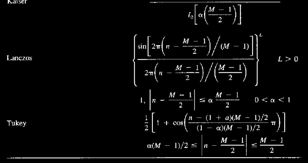
116 B.1 Windowing Functions-- Some Examples

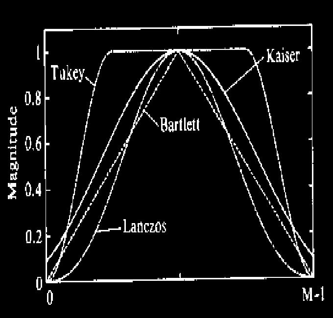
117 B.2 Windowing Functions-- Time Shape

118 B.3 Windowing Functions-- Performance

119 B.4 Windowing Functions-- Low-Pass FIR Filter Design with Windowing Rectangular Window(M=61) Hamming Window (M=61) Blackman Window (M=61) Kaiser Window (M=61)

120 Remark C: QMF/DCT/MDCT QMF h ( n) = h ( n) = 0 for n < 0and n N l u h ( n) = h ( N 1 n) n = 012,,, N / 2 1 l l h ( n) = h ( N 1 n) n = 01,,... N / 2 1 u n h ( n) = ( 1) h ( n) u u jω jω H ( e ) + H ( e ) = l l 2 2 u 1

121 C.2 DCT DCT IDCT F u N 1 2 n u ( u) ( u) x( n)cos ( = ) π α u = 01,,..., N 1 N 2N α( 0) = 1/ 2; α( u) = 1for u 0 2D DCT & 2D IDCT n= 0 N 1 2 n u xn ( ) ( u) F( u)cos ( = ) π α n = 01,,..., N 1 N 2N n= 0 N 1 N 1 2 n u m u F( u, v) ( u) ( v)[ x( n)cos ( = ) π cos ( ) π α α N 2N 2N n= 0 m= 0 α( 0) = α( 0) = 1/ 2; α( u) = α( v) = 1if u 0, v 0 N 1 N 1 2 m u n u xmn (, ) ( u) ( v) F( u, v)cos ( = ) π cos ( ) π α α N 2N 2N u= 0 v = 0

122 C.3 MDCT MDCT 2N 1 1 F( u) = h( n) x( n)cos ( u + )( n + + N) u,, n N = 01 = h ( N 1 n) = h ( n) = h ( N + n) + h ( 2N 1 n) = 2 for0 n < N. 1 π hn ( ) =± 2 sin ( n+ ) 2 2N