Working with Numbers: Excel 2007/10 Project 3: Format & Arrange

Transcription

1 Lesson Objectives Working with Numbers: Excel 2007/10 Project 3: Format & Arrange Use Page Layout view Format text - font, font color, font size Merge and center cells; unmerge Copy formatting - Format Painter, AutoFill, Paste Special Format part of text in cell Format a selection as a table with a table style Clear all formatting Apply a different theme Modify a table - size, options Sort and filter in a table; custom filter Print a selection Convert table to range Open an existing workbook Create and apply a cell style Merge cell styles from another workbook. Wrap text in a cell Customize the ribbon Format a chart - chart type, data series, fill, labels, titles, legend Move and copy cells and sheets Use Paste Special, Paste Link Insert cell, row, column, sheet Edit multiple sheets at the same time Print in Landscape orientation Print entire workbook Know the meaning of error values Previously, in Excel Project 2, you worked on spreadsheet basics - entering data, simple calculations, and printing your results. In Excel Project 3 you will learn to format your sheets to make them easier to read and use, by choosing the font, font size, color, and alignment. You will learn how to rearrange the parts of your workbook by moving, inserting, and copying cells, ranges, and sheets 1

2 Format & Arrange: Format Cells Adding formatting to your spreadsheet not only makes it more attractive, it can also make it easier to read and use. The right font, the right font size, the right color, and the right background can combine to make the most important information pop right off the sheet. Handling the blank areas is also important. Without enough "white space" (blank areas), your data can be hard to read. Columns and rows need to have some breathing space so your eye will see a break between them. Excel's sheets behave in many ways like Word's tables. There are some important differences, as you will see in this project. Word tables and Excel sheets look similar but do not behave quite the same. In this project you will apply formatting in several different ways. You will probably find that you prefer one approach, but you can not choose your favorite until you have seen them all! Below is a brief introduction to the formatting methods you will use in the Step-by-Step pages. Format Cells Dialog The Format Cells dialog has six tabs, each with several characteristics that you can set. 2

3 Number tab: Pick a number format and set its options, or create a custom format. Alignment tab: Horizontal and Font tab: Pick a font, font vertical alignment. Text control style, font size, font color, choices: Wrap text, Shrink to underline style, a few fit (the cell), Merge cells, plus effects. Orientation, which rotates text. Border tab: Set a border for any combination of edges of your selected cells plus diagonals. Fill tab: Background colors and patterns and special effects with gradients. Protection tab: Keep certain cells from being changed by someone using your sheet or even hide parts of the sheet. Your choices in this dialog apply to the whole cell unless you have selected only part of the contents of that cell. Some formats, like font and font size, can be applied to just some of the characters. Other formats, like Borders and Alignment, apply only to the whole cell. 3

4 Copy Formatting To copy formatting you can use one of the Paste Options, the Format Painter, AutoFill, or the Paste Special dialog. Paste Options: When you click the Paste button's arrow, a list of options appears. In Excel 2010 the choices are icons. Hover over an icon and a screen tip will tell you what it will do. If you just click the Paste button itself or use the key combo CTRL + V to paste, the Paste Options button appears near what you pasted. So you can choose before you paste or afterwards. Hurrah for flexibility! In Excel 2010, again there are icons to show you what choices you have about what you want pasted. Format Painter: The Format Painter button works much as it does in Word. The biggest difference is that Excel's Format Painter works only on the cell as a whole. You cannot use it on just part of the text in a cell. In fact, it is grayed out when you are in Edit mode. 4

5 When you click the button, the pointer changes to its Format Painter shape. Click on a cell or drag across several cells to apply the copied formatting. The pointer then returns to its Select shape. To use Format Painter to format several cells that are not next to each other, doubleclick the Format Painter button. The pointer will remain in its Format Painter shape until you click the button again or press the ESC key. If a cell contains more than one format for text, such as different font sizes, Format Painter will copy only the first formatting that it finds. AutoFill: You can use Excel's AutoFill feature to copy formatting into multiple cells, while leaving the data in the cells alone. AutoFill Options: After you drag the Fill handle to copy cells, the AutoFill Options button appears near the bottom right of the cells. Click its arrow to open the list of choices. You will see various choices depending on what you were copying, but you should always see Fill Formatting Only and Fill Without Formatting. Right Drag Menu: If you drag the AutoFill handle with the right mouse button, a menu automatically appears with the same choices, including Fill Formats. 5

6 Format & Arrange: Apply Formatting In Excel your formatting choices are on the ribbon but also are grouped neatly in a single dialog with 6 tabs. There are so many choices! It will take you a while to become familiar with all of them. In this section you will apply text formatting. Later you will work with number formats, alignment, borders, and fills. Default settings for Format Cells - Font tab 'Normal font' resets the dialog to the default font settings. 6

7 Paste Special: The Paste Special dialog ( Home tab > Paste >Paste Special ) allows you to choose how much about a copied cell you wish to paste. You can choose All and paste the entire cell with all of its formatting. Or choose one of the Paste options and paste just that characteristic. Of special interest for this project is the choice to paste just the Formats. You can even paste everything except the borders. This is very useful when some rows have borders and some don't. If you choose one of the Operations, the operation is performed on the pasted contents when you paste. Pasting multiple cells with Skip blanks checked leaves the data you are pasting over in place if the new data has a blank cell in that position. Transpose will paste columns as rows and rows as columns, which can be quite useful and certainly saves a lot of time. Clear Formats After all this formatting, what do you do if you want to just start over? How can you get rid of all these formats, called clearing formats? 7

8 Ribbon: On the Home tab, the Clear button opens a list of choices, including Clear Formats, which returns all the fonts to the default Normal font, removes fills and borders, and splits merged cells. It does not change row and column sizes. Data that was lost in a merge is not restored. 8

9 Step-by-Step: Apply Formatting What you will learn: to edit an existing header in Page Layout View to apply text formatting with dialog to apply text formatting with ribbon to merge cells and center cells to unmerge cell Start with: trips9-firstname-lastname.xlsx (saved in previous lesson) Edit Header: Page Layout View 1. Open trips9-firstname-lastname.xlsx from your Class disk in the excel project2 folder to Sheet1. 2. Switch to Page Layout view. 3. Edit the Right section to read Excel Project 3 4. Use Save As to save the file to the a new folder, excel project3, on your Class disk as trips9-titleformatted-firstname-lastname.xlsx. Create the folder excel project3 if it does not yet exist. 9

10 Format Cell: Dialog 1. Select cell A1 = World Travel Inc. 2. From the ribbon on the Home tab in the Cells tab group, click the button Format and then Format Cells... The Format Cells dialog appears, open to the Font tab. It has 6 tabs for formatting options. 3. Click on each tab to see what you can use it for. So many choices! Especially notice the choices on the tabs Number and Alignment. 4. Return to the Font tab. Cell A1 is still selected. 10

11 5. Make the following choices: Font = Matura MT Script Capitals Font Size = 24 Font Color = Blue, Accent 1, Darker 25% 6. Click on OK to close the dialog and apply your choices. Format Cell: Ribbon Some of the most common formatting choices are also available on the ribbon. Handy! 1. Select cell A2 = Anniversary Specials 2. On the Home tab in the Font tab group, use the buttons to format this cell as: Font = Arial; Font Size = 18; Font style = Bold; Font Color = Blue, Accent 1, Darker 25% 11

12 Format Cell: Merge and Centre 1. Select the range A1:E2, which is first two rows across the width of your data. 2. On the Home tab click the Merge and Centre button. You get a warning! When cells are merged, all data is lost except what is in the upper left cell. This is very different from the way Word handles merged table cells, where each cell's contents becomes a separate paragraph in the merged cell. At least Excel will warn you that you are about to lose data. 3. Click Cancel. Problem: Text in A2 vanishes If you clicked on OK in the message box, then all of the selected cells merge into a single cell but only the text from the first cell is kept. Solution: Undo immediately. 4. Select just A1:E1 this time - all on the same row. 5. Click on the Merge and Center button again. The text in A1 is centered across the selection. 6. Select range A2:E2. 12

13 7. Click the Merge and Center button. The text in A2 is centered over the selected range. 8. Save. [trips9-titleformatted-firstname-lastname.xlsx] Unmerge Cells: Ribbon & Dialog If you change your mind or have not selected the right cells to merge, you can unmerge in two ways - the ribbon and the Format Cells dialog. This section is just practice with no changes to save. Unmerge with Ribbon: 1. Click on the title, World Travel Inc., in the merged cell on row 1. The merged cell is selected. 2. Click the arrow beside the Merge and Center button. The menu opens. 3. Click on Unmerge Cells. The text moves back to A1 but it is still centered in that single cell. That makes part of the title hang out of view to the left. 4. Click in cell A3 to deselect. 5. Undo. 13

14 Unmerge with Dialog: 1. Click on the subtitle in row On the Home tab, click the dialog box launcher for the Alignment tab group. The Format Cells dialog opens to the Alignment tab. 3. Uncheck the box by Merge Cells. 4. Click on OK to close the dialog. The subtitle is back into A2 but still centered. 5. Undo. Add button to Quick Access Toolbar: If you find yourself doing a lot of unmerging or having to take out centering, you could customize your Quick Access Toolbar to include a Merge Cells button (without the centering) and an Unmerge Cells button. 14

15 Format & Arrange: Copy Formatting Once you have created a formatting scheme, you probably will want to use it on other cells. There are several ways to copy just the formatting. All methods apply to whole cells. If you want part of the text in a cell formatted differently, you will have to apply the formatting manually. Animation: Format B3 and copy the formatting to other cells Step-by-Step: Copy Formatting What you will learn: to copy formatting with Format Painter to copy formatting with AutoFill to copy formatting with Paste Special to resize columns to format only part of a cell's contents Start with: previous lesson) trips9-titleformatted-firstname-lastname.xlsx (saved in We will make things fancier using several different methods for copying formatting, just for practice. In the real world you would probably use only one at a time. Format Cell: Format Painter For quick copying of formatting, the Format Painter can't be beat! 1. Select cell A4 = Customer 15

16 From the Home tab, select : Font: Calibri Font Size = 14 Bold Fill = Dark Blue Font Color = White The row resizes automatically because of the larger font size. 2. While cell A4 is selected, click on the Format Painter button. The selected cell gets a blinking border. The pointer changes to the Format Painter shape. 3. Click on cell B4 = Trip. (Don't drag!) The formats from cell A4 are applied to cell B4 and the pointer returns to the Select shape. 4. Save As trips10-firstname-lastname.xlsx on your Class disk in the excel project3 folder. Keep Format Painter active: To use Format Painter on several cells in different places, double-click the Format Painter button. The pointer will stay in the Format Painter shape until you click the button again or press the ESC key. Then the pointer will go back to the Select pointer shape. Copy formatting for a range: Format Painter is smarter than it used to be. You can copy the formatting for a whole range and apply it to a range that is the same size or smaller. The pattern of formats will repeat for a range that is larger than the original range. Format Cell: AutoFill AutoFill is great for filling in a series of data but you can also use this feature to copy just the formatting. 1. With B4 selected, move the mouse pointer over the bottom right corner of the cell until the pointer changes to the AutoFill shape, a black cross. 2. Drag to the right until the next two cells are selected. The screen tip is showing that you are going to copy Trip into each of these cells. Don't panic yet! 16

17 3. Release the mouse button. B4. That's not what we want, of course. Cells C4 and D4 look exactly like The AutoFill Options button shows at the bottom right of the filled cells. 4. Hover over the AutoFill Options button to show its arrow. 5. Click the arrow to open this menu. 6. Click on Fill Formatting Only. The cell text goes back to the original but the formatting now matches cells A4 and B4. Slick trick! 7. Save. [trips10-firstname-lastname.xlsx] Format Cell: Paste Special The Paste Special dialog can handle several different ways to 'paste'. You can choose whether to paste everything or just the formula or just the current calculated value or just the formatting or a combination of some of these. 1. Select cell B4 and click the Copy button on the Home tab. The cell gets bordered with a blinking dashed border. The dashes look like they are chasing each other around the cell! 2. Click in E4. 17

18 3. On the Home tab, click the arrow below the Paste button to open its menu. The menu uses icons to show what can be pasted and in what format. Is it clear to you what each one will do? Problem: Paste button menu is different You must copy something first. Solution: Click on B4 again and then on the Copy button. Click on E4 and then on the Paste button arrow. 4. Experiment: Paste options Excel 2007: Try a choice in the list of Paste options. Undo and try another choice. Did the name of the choice make it clear what would happen? Excel 2010: Hover over each icon in the Paste menu. Guess what will happen. Live Preview changes cell E4 to show you what that choice would do. A screen tip tells what Paste would do. Did you guess right about each one? Some choices only affect numbers, not text. When you are ready to continue Select Paste Special at the bottom of the menu. The Paste Special dialog opens. This dialog has more choices! 6. Click on the Paste option Formats. Then click OK. 18

19 All of the formatting in cell B4 is applied to E4. 7. Press the ESC key to clear the blinking border around cell B4. 8. Save. [trips10-firstname-lastname.xlsx] Resize: Columns Notice that the row got taller when the text got a larger font size but the columns did not resize. The labels look crowded and C4 is cutting off some of the text. Let's fix that now. 1. Drag across the column headings C, D, and E. 2. Double click on the right edge of the column heading of one of the selected columns. All the selected columns are resized with AutoFit to be wide enough to read all the characters. Now the text in C4 shows completely. 3. Save. [trips10-firstname-lastname.xlsx] Format Cell: Part of Cell Text Sometimes you want part of the text in a cell to be formatted differently - color, italics, bold, font size, font,... whatever. 1. Double-click cell A2 to get into Edit mode. 19

20 The Status bar should show Edit. 2. Select the word Specials and click the Italics button. 3. While "Specials" is still selected, change the Font color to Red, Accent Click a different cell to save your change and remove the selection. 5. Save. [trips10-firstname- Lastname.xlsx] 20

21 Format & Arrange: Table Styles Excel makes it easy to format part of your sheet as a table by providing a number of table styles. The initial table styles have formatting for heading rows, borders, and alternating background colors for data. The colors are those in the current document's theme. Apply a table style: Table Styles Gallery Select the cells that you want to be in the 'table' first. Select a style from the gallery of table styles. Excel adds arrows for each column when you apply a table style, but, happily, those arrows won't print. An arrow opens a menu of sorting and filtering options for the table based on that columns. Remove a table style: Clear formatting Hide the sort/filter arrows: With at least one table cell selected, 0n the Data ribbon tab, click the Filter button to turn it off. The column arrows go into hiding. Not an obvious thing to do! There are times when you regret you ever started formatting. You want to start over with no formatting at all. Undo works if you are willing to back up. But Undo remembers only the last 100 actions. The Clear Formatting command on the Clear button will remove what the table style applied, but will not clear formatting that you applied yourself. In older versions of Excel, what is now called a table was called a list. 21

22 Step-by-Step: Table Styles What you will learn: to format with table style to clear all formatting to change theme Start with: trips10-firstname-lastname.xlsx (saved in previous lesson) 1. If necessary, open trips10-firstname-lastname.xlsx 2. Save as trips11-firstname-lastname.xlsx in the excel project3 folder Format Cells: Table Style It is usually helpful to use different formatting for column and row labels and rows and columns that have totals. Excel has a larger number of table styles that use the theme colors and fonts to help with this. A 'table' in Excel is not just the whole spreadsheet, and it is quite different from a 'table' in Word. 1. Select the range A4:E25, which is the upper table on the sheet. 2. On the Home tab in the Styles tab group, click the button Format as Table. 22

23 The gallery of table styles opens. How do these styles differ? o Different colors from the document theme o Format for header row different from data row o Alternating color bands for rows o Borders around rows or all cells, or no borders at all. Live Preview does not work for the gallery from the Format as Table button to start with. But once you have applied a style, Live Preview does show the effect of the style your mouse is over. New Style: The gallery of table styles includes a command for New Table Style... but such a new style will not show up later in the gallery for a different document. So sad... and annoying! 3. Select the style named Medium 2. A dialog appears showing what cells will be in the table. Be sure that the box is checked for My table has headers. 4. Click on OK. The dialog closes, the style is applied to the table, the ribbon changes to 23

24 the tab Table Tools: Design. What changes in the table itself? o The header row gets arrows. o The data rows have alternating bands of background fill. o The header row did not change formatting even though the color and font size are different from the Medium 2 table style. 5. Experiment: Table Style With the table still selected, on the Table Tools: Design tab, hover over several different styles in the Table Styles gallery, but do not click(!). Click the More button to see the full set of styles. Live Preview works now to show you how the style you are hovering over would change the formatting of the table. Examples: Dark 10; Dark 7; Medium 15 The header row is not changing to match the style! That is because earlier you applied formatting manually to those cells - font, font size, font color, fill color. For the table style to change cells that were already formatted, you have to remove that manual formatting. When you are ready to continue Save [trips11-firstname-lastname.xlsx] Clear Formats The Clear button on the Home tab has choices for what to clear, including just the formatting. Just what you need right now. You did that manual formatting for row 4 a long time ago. Undo cannot help this time! 24

25 1. With the table still selected, on the Home tab in the Editing tab group, click on the Clear button. The menu of choices opens. Clear All will remove the formatting and the contents of the selected cells, too! 2. Click on Clear Formats. The selection goes back to the default formatting for the sheet. The arrows stay in the header row. The cells are still part of a 'table'. Alternate Method: Right click on a table style thumbnail and select Apply and Clear Formatting. This has the advantage of doing two things with one click! 3. Experiment: Table Style 25

26 o Try out several styles using the Table Styles gallery on the Table Tools: Design tab. Now the header row changes with the table style. Examples: Dark 10; Dark 7; Medium 15 Now the header row is changing with the table style. 4. Apply Medium 2 again. The header row is similar to what you applied manually before, but the fill color is a bit lighter and the font size is smaller. You lost the accounting formatting for the 'Total sale' column. 5. Switch to the Data ribbon tab. The Filter button is highlighted. 6. Click the Filter button. The column arrows are hidden. The cells are still a table. You can get them back by clicking the Filter button again. 26

27 7. Save. [trips11-firstname-lastname.xlsx] Change Theme The Themes gallery is big and hides a lot of your sheet. You need to use a smaller document window so you can see what Live Preview does to the document. 1. Click the Restore button for the document. This button is at the top right of the Excel window, below the controls for the Excel window. The workbook window resizes. 27

28 2. Drag the workbook window to the right to leave room at the left for the Themes gallery. 3. On the Page Layout tab, click on the Themes button. A gallery of themes opens. You will have to scroll to see them all. If you have not done the Working with Windows lessons, your gallery will not have the Sun-Tahiti theme that is in the illustration. 4. Experiment: Theme Hover over but do not click on various themes to let Live Preview show what would change in your sheet. Examples: 28

29 29

30 What changed? o o o Fill colors for bands and header row Font & font sizes for cells Colors for titles (which were selected from theme colors) What did not change? o o o o Fonts and font sizes that were manually applied (Title and subtitle) Font styles that were manually applied (Italics for 'Special') Alignment (Center in lower rows) Merged cells (Title and subtitle) When you are ready to continue... 30

31 5. If necessary, return the theme to Office. 6. Click on the Maximize button for the worksheet window so that the window takes up all of the workspace again. 7. Save. [trips11-firstname-lastname.xlsx] 8. Close the workbook. 31

32 Format & Arrange: Modify Table Excel table style thumbnails show just a header row and alternating colors for the row. Once you have defined a table, the Table Tools: Design tab lets you choose several other features for your table style to manage. You can mix and match these options and the style thumbnails will automatically update. Some table styles do not format all of the options. You can rearrange your table by sorting on any column. Sorting multiple times in a sequence can work well or give very unhappy results, depending on your choices! Applying a filter will hide rows that do not match your criteria. For example, in a table of orders, you could filter to see orders from a particular person or company. Or perhaps you are looking for a particular order that was for $ but you cannot remember who placed the order. A filter on the order's total would hide all orders for other amounts. The orders are not removed from the spreadsheet. They are just hidden while the filter is in place. Table styles are part of each Office theme. A theme sets the default colors, fonts, and effects for objects. Changing a theme automatically updates your document IF you originally chose from the colors, fonts, and effects that were in the theme. Office 2010 has more pre-designed themes than Office 2007 has. 32

33 A custom theme that you created shows at the top of the gallery of themes. If you did the Working with Words lessons, you created one, Sun-Tahiti. A custom theme is available for any new Office document, not just the program you were in when you created it. Step-by-Step: Modify Table What you will learn: to change a table's size to change table style options to sort and filter with table columns to create a custom filter to print a selection of a sheet to convert a table back to a range Start with: trips11-firstname-lastname.xlsx (saved in previous lesson) 1. If necessary, open trips11-firstname-lastname.xlsx 2. Save as trips12-firstname-lastname.xlsx in the excel project3 folder Change Table Size You can modify several features of your table, like the size and whether or not there are special rows or columns. The bottom right cell of the table has a symbol in its bottom right corner. When you hover over this corner symbol the mouse pointer changes to the diagonal resize shape. You can drag to increase or reduce the cells included in the table. Table style formatting will change as you drag the table larger or smaller. 33

34 1. Size o o o o o Experiment: Change Table Click out of the table so you can see the corner symbol. Drag the bottom right corner of the table up a few rows and release the mouse. Drag the bottom right corner back down. Drag left and then click out to deselect the table. Can you drag up and left at the same time? Down and right? What formatting changes? When you are ready to continue... return the table to include A4:E25. If you get a warning about a circular reference, use Undo to return your table to its original state. 34

35 Change Table Style Options 1. Click in the table somewhere. The tab Table Tools: Design appears again. The tab group Table Style Options has check boxes for special types of rows and columns. The table styles already include formatting for these special features. The default table styles include a Header Row and Banded Rows, so those boxes are already checked. Some of the styles do not have special formatting for some of the options. The thumbnail cannot show that a column will be Bold or what font will be used. 2. On the tab Table Tools: Design in 35

36 the Table Style Options tab group, click the box by First Column. What changed? The first column of the table became bold. The thumbnail you saw did not show this. 3. Click on Last Column and Banded Columns. The last column turns bold. Alternate columns have colored fill now, just like the rows did. The effect can be rather odd, depending on the widths of the columns involved. 4. Click on the box by Total Row. This is not a change in formatting! A new row appears at the bottom of your table, outside the table border. This works well ONLY when you did not already have a totals row!! Look at the value in row 26. It is double the lovely sum you already had in row 25. Clearly the total in the new row is adding up everything in the last column, including the total that was already there. Bad idea for this table!! This new total row creates only a total for the last column. If you want other totals, you can create them on this row. Use the Total Row option when you do not already have a totals row for the table. This is especially useful when you want to look at how some totals change as you filter the table temporarily. 5. Experiment: Special Rows and Columns Try out several combinations of the choices in Table Style Options and various table styles. Which do you think would work well with this particular table? When you are ready to continue Uncheck the boxes for Total Row, First Column, Last Column, and Banded Columns. You should be back to the formatting you started with. 36

37 It is not necessary to save since no changes were kept. Sort Table The header row (row 4) gained a drop list for each column. Each arrow opens a menu of choices for sorting and filtering the whole table based on what's in that column. Sorting rearranges the rows. Filtering hides the rows that do not match the criteria that you pick. 1. Click outside the table to deselect the table. The column arrows did not disappear! This is one of the benefits of setting up cells as a table. You do not have to select the table again to use the commands on the arrow menu. 2. Click the arrow for the first column to drop its menu. You have several sorting choices and filtering choices. 3. Select Sort A to Z. What changed? o Rows moved into alphabetical order by Customer name. o Arrow button: has an up arrow. 37

38 o Original Totals row: Sorted with other rows. The calculated values changed! This could be a problem! There is a green triangle in the corner that show there IS a problem. Click in cell E21 and then click on the error icon to see the message. Look at the Formula bar. It shows =SUM(E2:E21) but the last customer row is row 24. Moving the formula is making a mess! Leave your own totals row out of the 'table'. Then it won't be sorted! o Table formatting: Did not move with the data. That's a good thing! 4. Open the Customer column list again and select Sort Z to A. What changed? 38

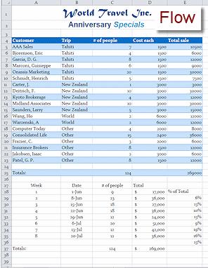
39 o Rows moved into reverse alphabetical order by Customer name. o Arrow button: has a down arrow. o Totals row: Moved again and got new values. Wow! Quite a change! The formula is adding up only the cells above it. o Table formatting: Stays in place. Did not move with the row. 5. Undo twice! Your table should be back the way it was before sorting, with the custom sort by trip with Tahiti first. Do not include a formula when sorting unless ALL relative cell references in the formula are to cells in the same row. 6. Experiment: Sort o Sort using other columns. Exactly what choices you see in the menu depends on the kind of data in the column. o Click on Sort by Color. You will see choices here only when you have applied colored fill in cells with Cell Styles (which we will look at in a later lesson). The background fills from the table's style do not count. The Sort by Color choice also includes a link to the Sort dialog where you can sort on multiple columns, as you did in an earlier lesson. When you are ready to continue Undo all of your experimentation. You should be back to how the table was formatted at the beginning of this topic. Filter Table: Match Existing Values The choices in the Filter section of the menu depend on whether the data in the column is text or numbers. Once of the most common filters looks for one or more values that are known to be in the column. Those value show in the menu from the column's arrow. 39

40 1. Click the arrow for the Trip column to open its list. 2. Click the (Select All) box to deselect all values at once. 3. Click on New Zealand and World. 4. Click on OK to apply the filter you just created. What changed? o Rows do not move but are hidden. Look at the row headings. Numbers between 15 and 26 are missing! Only rows with a Trip value of New Zealand or World are visible. o Arrow button: gained a funnel, which is the symbol for a filter. o o Totals row: Vanished. Table formatting: Applied to the visible rows. Does not follow the data rows. 40

41 5. Click the filter button on the Trip column again. 6. Click Clear Filter From "Trip". The full table reappears. 7. Experiment: Filter Try out filters on different columns and clear them. What happens when you filter two different columns without clearing the first filter? 8. Use Undo multiple times to return the data to the original arrangement - Sorted on the Trip column with a custom list, with Tahiti first. Filter Table: Logical Test Sometime you want to see the rows where the values are less than a particular number, or greater than a certain value. Or you might want to search for values that start with a particular text. 41

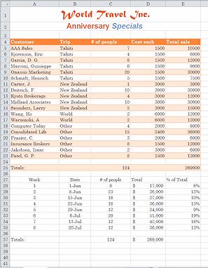
42 1. Click the arrow on the column Total sale. The Sort and Filter menu appears. 2. Hover over Number Filters to expand its submenu. If the column contains text, you would see Text Filters instead. 3. Click on Greater Than Or Equal To... The Custom AutoFilter dialog opens, with the first text box already filled in with a logical test: is greater than or equal to. 4. Click the arrow in the text box at the top right. A list of values in the column appears. 5. Click on When 'And' is selected, both criteria must be met. When 'Or' is selected, only one must be true, but it is OK if both are true. 42

43 6. Click the arrow beside the the second logical test and scroll the list to see all of the possibilities. Do not choose any of these at this time. 7. Click on OK to close the dialog and apply your filter. Only 5 rows of data and the Totals row still show. They are the only ones with a Total sale value of 15,000 or greater. 8. Experiment: Custom Filter Try out other choices for a custom filter. What happens when you combine filters with AND selected in the dialog? What happens when you combine filters with OR selected? When you are ready to continue Clear the filter. Your table is back to its original status. Print Selection You can print just part of a spreadsheet by setting the Print Area, but that is permanent until you change the print area. For a temporary situation, it's better to select what you want to print and use the Print choices to print only that selection. 43

44 1. Select the range A1:E25. This is the upper table and the title and subtitle. 2. Excel 2007: Click the Office button and Print. In the Print dialog, click the radio button for Print Selection, then click on Print Preview. Excel 2010: Open Print Preview. Change the settings, if necessary, to Print Selection. 3. Verify that only A1:E25 will print! Notice that the column arrows do not print! Yeah!! 4. If necessary, change orientation to Portrait. 5. Save. [trips12-firstname-lastname.xlsx] Convert Table to Range Are you annoyed by those arrow buttons on each column? Once you get your table sorted, you can return the cells to an ordinary range, but the formatting and the sort order stay in place. Filters will be cleared automatically when you convert the table back to a range. 44

45 Here is a fast way to remove all the cell formats and get back to basics - Normal font, no borders, no fills, no merged cells. To return to a previous stage in your formatting, you can use Undo. But Undo only remembers 100 actions. That sounds like a lot, but you can easily exceed that number in a single editing session! 1. Switch back to Normal view and open the Name Box list. 2. Click on Table1. Your list will show a different number if you created a table more than once during your work. The whole table appears to be selected, but the header row is outside the border. It is hard to see blue highlighting when the table colors are blues. 3. On the Table Tools: Design tab in the Tools tab group, click on the Convert to Range button. A message box asks if you want to convert the table to a normal range. 4. Click on Yes. The columns arrows are gone but the table style formatting and sorting order remains. Any filters would be removed automatically. Now that we are finished with table styles, let's get our formatting back on 45

46 those amounts of money. 5. Apply Accounting style to E5:E23 and E25, with no decimal places. 6. Save. [trips12-firstname-lastname.xlsx] Clear All Formats One of the common uses for tables is to apply a table style for formatting. But suppose you need to get rid of that formatting later? You can clear the formatting in several ways. 1. In the Name Box, type A1:E25 and press ENTER. This selects all of the cells that you have been working with lately. 46

47 2. From the Home tab in the Editing tab group, click the Clear button and then Clear Formats. All formatting is removed from the selection... except for the word 'Specials'. Unexpected! Because the formatting was not applied to the whole cell, it is not removed by Clear Formats. You could manually change each format or else delete the word and retype it - which is easier! 3. Save as trips12-clearformats-firstname-lastname.xlsx to the excel project3 folder 4. Open Print Preview. Problem: Preview is blank except for the header What happened?? Your print settings are still set to Print Selection. 47

48 Solution: Change the setting for the printer to Print Active Sheets. 5. Close the spreadsheet. Format & Arrange: Cell Styles All this work with table styles brings up a question. Does Excel have other kinds of styles, like Word has character and paragraph styles. Yes, indeed! Excel uses cell styles instead of character or paragraph styles. They make it easy to format different cells alike when you don't need a whole table. A cell style, or just style, can include any formatting that can be set for a cell. This includes all of the font characteristics, number formats, alignments, fills, and borders. Excel provides some pre-defined styles in the Styles gallery on the Home tab. You can also create your own custom cell styles. What is a cell style good for? 48

49 To quickly apply formatting to cells that you want to emphasize in a special way. To automatically update the formatting everywhere the style was applied whenever you modify the style. You avoid having to hunt around for the cells that need the same styling and then having to fix them individually. Automatically updating things is what Excel is all about! Step-by-Step: Cell Styles What you will learn: to open an existing workbook to create a cell style to apply a cell style to check what style a cell has to modify a cell style to merge cell styles from another workbook to wrap text Start with: trips12-firstname-lastname.xlsx (saved in a previous lesson) Open an Existing Workbook There are many ways to open an existing file. Recent file: o Start menu > Recent Items o Taskbar icon - right click > Recent o Inside Excel: Office button menu > Recent Documents or File tab > Recent Computer window showing your Class disk, folder excel project3 49

50 Start menu > Recent Items; right click pinned Excel icon > Recent; File tab > Recent; My Computer window > excel project3 1. Open trips12-firstname-lastname.xlsx from your Class disk. 2. Save as trips13-firstname-lastname.xlsx. Create a Cell Style The first cell style you will create will duplicate the formatting in the header row, row 4. You could apply the same table style to the bottom section of data, but that pulls is a lot of features that are just not needed for such a small table. Besides, this lesson is on cell styles! 50

51 1. Select cell A4 = Customer This cell got its formatting from the table style Medium 2, but you converted the table back to a range. 2. On the Home tab in the Styles tab group, click the More button to show the gallery of cell styles. Styles are in groups: Good, Bad, and Neutral; Data and Mode; Titles and Headings; Number Format. When you have created custom styles, they are at the top in a new section, Custom. 3. Click on New Cell Style... The dialog shows the formatting for the current cell, A4. 4. Type a new Style name in the box: Header Row The dialog includes a list of how the selected cell is styled. It is nicely detailed, except for Fill, which does name the color. An odd omission! 51

52 5. Click the Format... button. The Format Cells dialog appears, where you can view or modify all of the settings. You don't need to modify anything right now. 6. Click on each tab in this dialog and notice what the choices are and what the current choice is. By the way, on the Font tab, the Preview box looks like it has no sample text. The font color is White, so the text is there, as white text on a white background. Invisible! 7. Click the OK button to close the Format Cells dialog. 8. Click on OK again to close the Style dialog. The new style appears in the gallery on the Home ribbon tab, listed first. 52

53 Apply Cell Style 1. Select range A27:E Click on the cell style Header Row in the gallery of cell styles. Which Style? You cannot tell by looking whether or not a cell has a cell style applied to it. The Style gallery comes to the rescue! 1. Select cell E Look at the Styles gallery on the Home tab. The style with the gold border is the current style, Header Row. Modify Cell Style 1. Right click on Header Row in the Styles gallery. 53

54 A menu appears. 2. Click on Modify Style... The Style dialog appears. 3. Click on the button Format... The Format Cells dialog appears, open to the Font tab. 4. to Cambria and the Font Size to 14. Change the Font 5. Click on OK to close the Format Cells dialog. The Style dialog now shows the new Font settings. Live Preview does NOT show what effect this change will have. 54

55 6. Click on OK to close the Style dialog. The Style gallery shows the new formatting. All cells in row 27 to which you applied the Header Row cell style are using the new formatting. Sweet! What about the cells in row 4 from which we got the formatting? No, they stayed the same! You never applied the cell style to them. 7. Save. [trips13-firstname-lastname.xlsx] Merge Cell Styles Your new custom style is not seen by other workbooks. You can use the Merge Styles command at the bottom of the Styles menu to import styles from another workbook. Both workbooks must be open before you use that command. You can merge styles even if they have the same name. 55

56 1. Open the following workbook: styles-merge.xlsx from the resources for working with numbers link. 2. In trips13-firstname-lastnme.xlsx make Sheet 1 the active sheet. 3. Click the More button for the Styles gallery. 4. Click on Merge Styles... at the bottom of the gallery. The Merge Styles dialog opens. The dialog lists the other open workbooks. 5. Click on styles-merge.xlsx to select it. 6. Click on OK to close the dialog. The Styles gallery now shows two new styles in the Custom section, Dates and Totals. Notice that your custom cell styles are listed first, in alphabetical order. 7. Save. [trips13-firstname-lastname.xlsx] 56

57 Apply Cell Styles 1. Select B28:B35, the dates in the bottom table. 2. Click on the Dates cell style to apply it. 3. Select cells E25 & D37, the total sales. 4. Apply the Totals cell style. 5. Save. [trips13-firstname-lastname.xlsx] Wrap Text When your text is too long to fit in the cell's width, you can force the text to wrap inside the cell. This is often better than just widening the column enough for the text to fit. 57

58 1. Select cell C4. 2. Type Number of people This replaces the existing text, # of people. 3. Similarly, replace the text in cell C27 with Number of people. In both C4 and C27 the text is cut off at the right. 4. Select C4 and C27 at the same time. (Hint: Hold CTRL down when you click the second cell.) 5. On the Home tab in the Alignment tab group, click on the button Wrap Text. Rows 4 and 27 immediately get taller to hold a second line of text. The text is still aligned Left. 6. Save. [trips13-firstname-lastname.xlsx] 58

59 Format & Arrange: Format Chart Once you have created a chart, you are not locked into your choices forever. You can change everything about the chart. Of course, if you have several changes, it might be faster to just start over. The chart type determines the basic look of your chart - column, line, pie, bar, area, scatter, ring, doughnut, etc. In addition the chart type will set font styles and sizes for titles and data labels, colors and patterns, gridlines, scale on the axes, and other features of your chart. The predefined chart types provide a very useful shortcut to chart design. You can customize any of features and save your design as a Custom type. Commands for formatting charts are available on the Chart Tools ribbon tabs (Design, Layout, Format). Some commands are also on menus that pop up with a right-click on chart parts. Sometimes it can be hard to click in just the right spot to get the menu you want. Use the ribbon for the basics. That's the easy way! Parts of a Chart It might help to know the parts of a chart before you try to format one. Some types of charts do not have all of these parts. For example, a pie chart does not have axes. 59

60 Plot area Data series Data point Data label Axis Data table Chart area where the data is actually pictured the bars or dots or wedges that represent the values you are charting a single value represented by a bar, dot, or wedge in the chart a label for a bar or dot or wedge, displayed near it on the chart, showing the name, value, or the % of the whole the vertical or horizontal edge of the chart that is marked off in even lengths a table of the values plotted on your chart includes all of the chart parts - the plot area, the titles, the data table, legend, and background Background the color, pattern, or image behind the actual chart Titles Legend Chart tips the title for the whole chart and titles for each axis shows what the colors or patterns on the chart represent a screen tip that identifies the part your pointer is over. For a data point, the screen tips includes the name of the data series, the row label for the data point, and the data point's value. 60

61 Format & Arrange: Format Pie Chart Pie charts are most useful for showing how the parts relate to the whole. In the sample chart below, the sizes of the wedges give you a quick feel for the relative sizes - which pieces are biggest, which are smallest, which are about the same size, which parts make up the bulk of the whole. You get more exact numbers when you include the values or the percentages as part of the data label. Sample Pie Chart Step-by-Step: Format Pie Chart What you will learn: to format chart title to explode a pie chart to explode one wedge of a pie chart to format data points Start with: trips13-firstname-lastname.xlsx (saved in previous lesson) Format Chart: Title In the previous lesson Basics: Chart, you created a pie chart for the number of tickets sold for each week that World Travel Inc. had their special offers. Now you will learn how to make changes to the formatting. 61

62 1. Open trips13-firstname- Lastname.xlsx from your Class disk in the excel project3 folder, if it is not still open. 2. Save As trips14-firstname-lastname.xlsx in the excel project3 folder on your Class disk. 3. Select the sheet named Pie Chart-People. 4. Click on the chart's title to select it. When you changed the column label from # to Number, the chart was updated automatically. Cool feature! 5. Use the Formatting bar to format the title as: Font = Britannic Bold Font Size = 16 not Bold 6. Save. [trips14-firstname-lastname.xlsx] Format Chart: Explode Whole Pie or Part 1. Click on the pie to select it but do not release the mouse button. Be sure that there are sizing handles around the edges of the pie. The pointer changes to the Move shape 2. Drag away from the center of the chart. You have exploded the whole pie! Problem: Only one wedge moves 62

63 You selected just one wedge by releasing the mouse button when trying to select the whole pie. Solution: Click out of the chart and then click on the pie again but do not release the mouse button until after you drag. 3. Drag back to the center to glue your pie back together. 4. Click on the red wedge labeled 19% to select it. This is wedge with the largest percentage. 5. Drag the selected wedge up and to the right a little. You've "exploded" a piece of the pie. This is a handy way to emphasize a special part of a pie chart. 6. Save. [trips14-firstname-lastname.xlsx] Format Chart: Data Point Each value in the sheet that is a wedge in the pie is called a Data Point. You can change the formatting for all or for just selected ones. Be careful when changing color assignments. Excel carefully places colors next to each other that won't look the same if printed in gray scale. You can make your chart unreadable with the wrong choices. 1. Right click on the dark red 19% wedge and choose Format Data Point from the context menu. 63

64 A dialog appears with several pages. Choices made in this dialog apply only to what is selected - the data points. 2. Experiment: Formatting Data Point Try out different colors and fill effects. Live Preview shows what the choices in this dialog will do. If you open a second dialog, such as for Colors, Live Preview will not update until you are back in the Format Data Point dialog. Try some changes for Border Color and Border Styles. When you are ready to continue, use Undo to return your pie to its original condition. 3. On the Fill page of the dialog, click on Solid fill and then open the Fill Color drop list for colors. 4. Click on More Colors... The Colors dialog appears. 5. If necessary, click on the tab Standard Colors. 6. Click on the purple hexagon on the 5th row, 2nd from the right. 64

65 7. Click on OK to close the Colors dialog and then on OK again to close the Format Data Point dialog. Your wedge now is colored with the purple that you selected. 8. With the chart selected, create a header like the one on the first sheet. Your name and the date on the left, the workbook name and sheet name in the middle, and Excel Project 3 on the right. 9. Open the Print Preview. The chart is centered horizontally and vertically on the page. 10. Change the page orientation to Landscape. The chart is sized to fill the page because the chart was selected. Excel 2007: Click on the Page Setup button and select Landscape on the Page tab. Click on OK to close the Page Setup dialog. Excel 2010: Click the Orientation button to the left of the preview and then click on Landscape. 65

66 11. Close the preview. 12. Deselect the chart by clicking on a cell somewhere else on the sheet. 13. Open Print Preview again. This time the chart covers only a part of the page. This page will print much faster and will use less ink! Excel 2010: But wait! What happened to the header you just created? Did it vanish? When you created the header with the chart selected, you did not create a header for the whole sheet! Surprise! 14. Open Page Setup and create your standard header: Your name and the date on the left, the workbook name and sheet name in the middle, and Excel Project 3 on the right. 15. Save. [trips14-firstname-lastname.xlsx] 66

67 Format & Arrange: Format Column Chart Column charts are good at showing how the data points relate to each other, instead of to the whole. It is much easier to see how each column compares to the others than it is to compare the wedges of a pie chart to each other. Plus, a column chart can compare different series of data to each other. A pie chart cannot do that at all! Example: Sheet with two charts - single series and three series First chart: Uses Total column. Compares totals to each other. Second chart: Used B4:D8. Groups values for Day 1, Day 2, Day 3 67

68 Step-by-Step: Format Column Chart What you will learn: to change chart type to format chart area with background texture to format plot area to format chart area with photo Start with: trips14-firstname-lastname.xlsx (saved in previous lesson) Change Chart Type 1. Open trips14-firstname-lastname.xlsx from your Class disk in the excel project3 folder, if it is not still open. 2. Save As trips15-firstname-lastname.xlsx in the excel project3 folder. 3. Right click in a blank area of the chart and choose Chart Type from the context menu. The Chart Type dialog opens. 68

69 4. Select Column, which is Excel's default chart type, and choose the first sub-type, Clustered Column. 5. Click OK. The chart is redrawn as a set of columns, using the default settings for this chart type. The data points are now labeled with the values they represent instead of the percentages. The 19% wedge for Week 2 now is labeled 23 but it retained the color you assigned to its pie wedge. All the other wedges are converted to the default dark red columns. The legend does not accomplish much since there is only one series of columns. You will get rid of it shortly. Since Week 2 had the highest number of tickets sold, it actually works well to have it's column a different color from the rest. 6. Save. [trips15-firstname-lastname.xlsx] Chart Area: Add Texture Background The blank background is good for many charts, but sometimes a pattern or image can make your chart more attractive. You do have to be careful that the chart remains easy to read. 69

70 1. Right click in a blank area of the chart and choose Format Chart Area from the context menu. The Format Chart Area dialog opens to its first page, Fill, with the Automatic radio button selected. 2. Experiment: Fill Try out other choices on the Fill page for fills. Live Preview works once you have made a selection. Try different solid colors, gradients, pictures, and patterns. When you are ready to continue Click on the radio button Picture or texture fill. More choices appear below the radio buttons. 4. Click on the Texture button to open its gallery. 5. Click on Blue tissue paper on the 4th row down. 6. Click on OK to close the dialog. 70

71 Your chart now shows a repeating blue textured image as a background. Much prettier than a plain white background! Of course a busy or dark image could make it hard to read your chart. 7. Save. [trips15-firstname-lastname.xlsx] Remove Legend The Chart Tools: Layout tab has buttons which open lists of choices for formatting various parts of a chart. None is the first choice on all of these buttons. You can also select the part you don't want and press the DELETE key. The ribbon is an improvement over earlier versions of Excel where these choices were buried in a tabbed dialog. 71

72 1. If necessary, select the chart again. 2. On the Chart Tools: Layout ribbon tab in the Labels tab group, click on the button Legend. A list of positions for the legend appears. 3. Experiment: Legend Inspect the icon beside each choice. The icons show a sample of the legend's position. Try out each one. Click on More Legend Options... to open the Format Legend dialog. Try out various combinations. The current chart is not really helped by a legend at all since there is only one data series. When you are ready to continue Click the Legend button again and click on None. The legend vanishes, but the text box Week that you added to label it remains. Alternate method: Click the legend on the chart to select it and press DELETE.) 5. Click on the text box containing Week to select it. 72

73 6. Press the DELETE key. The text box is gone and the plot area expands to take up the space. 7. Save. [trips15-firstname-lastname.xlsx] 8. Experiment: Other chart parts Try out choices on the buttons on the Chart Tools: Layout tab in the tab groups Labels, Axes, and Background. You can hide or reveal all of these parts of a chart. You can format many features, including background and lines. Use Undo to return your chart to its previous state. Edit Text on Chart You can edit the title and axis labels on a chart directly on the chart or in the Formula bar. Your typing will replace all of the text unless you select part of it first. 1. Click on title of the chart, 'Number of people'. You want the text box selected, not the text. That way your typing will replace this text. 2. Type Number of Tickets Sold, which will show in the Formula Bar. 73

74 3. Press the ENTER key or click out of the chart. Your typing will replace the existing text. The new text shows in the Formula Bar only at first. It shows in the text box after you press ENTER or click out. This text explains the chart better and has more appropriate capitalization. Alternate method: Select the title's text box and then drag inside the text box to select the text. Your typing shows directly in the box. This is a good method for editing text in place. Some people have trouble with the selecting. In that case, you can edit in the Formula Bar. 4. Save. [trips15-firstname-lastname.xlsx] Show Labels There are many parts that can be on a chart, but may not be on the layout you picked to start with. The ribbon makes it easy to add the ones you need. 1. On the Chart Tools: Layout ribbon tab in the Labels tab group, click on the button Axis Titles. A menu appears with only two choices. 2. Hover over Primary Horizontal Axis Title to expand its submenu. 3. Click on Title Below Axis. A new text box appears below the horizontal axis (the X-axis). The text in the box is not helpful = Axis Title. You will change that shortly. 74

75 4. Click on the Axis Titles button again and hover over Primary Vertical Axis Title. The menu that opens has more choices. Look carefully at the icons. Can you tell what each choice will do? 5. Click on Rotated Title. A new label appears to the left of the vertical axis (the Y-axis). Letters in the box run from the bottom to the top and are rotated compared to the rest of the chart. 6. Save. [trips15-firstname-lastname.xlsx] 75

76 Edit Text on Chart 1. Since the title for the vertical axis, Y-axis, is already selected, type Tickets Sold and press ENTER. Your typing shows in the Formula Bar until you press ENTER. Then it replaces 'Axis Title'. 2. Click the box for the title of the horizontal axis (X-axis) and type Week of Special Offer 3. Click out of the text box to enter your change. The font size seems a bit small compared to the title and the size of the columns. 4. Click on the vertical axis title. 5. On the Home tab, click on the Increase Font Size button twice. The plot area resizes to be narrower as the title takes up more space. 6. Click on the horizontal axis title and do the same. Again the plot area resizes. 7. Save. [trips15-firstname-lastname.xlsx] Edit Sheet Tab and Print 1. Change the name of the sheet from 'Pie Chart' to Tickets Sold Chart Hint: Right click on sheet tab and choose Rename or double-click the tab and type.) 2. Deselect the chart by clicking off the chart. 76

77 3. Open Print Preview. The preview is not in gray scale, even if the printer is set to print that way. This makes it hard to be sure what the printed page will look like. Notice that the bars all come out the same shade of gray! 4. Save. [trips15-firstname-lastname.xlsx] 77

78 5. Save a print screen and paste it onto a word document, then save it into your project 3 folder. Format & Arrange: Arrange You often think of a better way of arranging things just about the time you are nearly finished with your spreadsheet. Or, after you have used the spreadsheet awhile, you see that you need a more convenient way to arrange the data. Rather than starting over from the beginning, it is easier to move your data. Excel makes it easy to move, add, delete, and copy rows, columns, or selected cells - without messing up your lovely formulas. Of course, there are a few oddities you need to understand. Multiple ways to move: Cut and paste/copy and paste o o o Right click menu commands Shortcut key combos: Cut: CTRL + X Copy: CTRL + C Paste: CTRL +V Ribbon buttons o o Drag selected cells onto blank cells - no problem onto cells that already have contents: choose to replace or to move those cells. 78

79 You can only shift the existing data to the right or down. This means you must think before you move. Format & Arrange: Move It is rather amazing how often you need to move a row or column on your spreadsheet. Fortunately Excel makes this easy to do. You do have to plan ahead, however. If you are not careful, you may overwrite other cells and lose their data. Animation: Moving a row (loops 5 times) Refresh the window to replay the animation. When you want to shift a row or column without losing the existing data, you must move the existing cells either right or down. Those are the only choices. Step-by-Step: Move What you will learn: to move by dragging to empty cells to move by cut and paste to move cells to non-empty cells to move with right drag to move with menu commands 79

80 to move a sheet Start with: lesson) trips15-firstname-lastname.xlsx - Sheet1 (saved in previous Whether you are moving a single cell, a range, a row, or a column, the same methods apply. The method you choose will depend on whether the destination is blank or already has data and on whether you want to replace the data or move it aside to insert the new data. To practice moving data, you will first move the some columns away from the lower table. Then you will put the table back together again by moving its other columns. You will switch the positions of the Customer and Trip columns in the upper table and then the positions of the Week and Date columns in the lower table. Your final move will be to move the sheet Tickets Sold Chart. Move: Drag to Empty Cells 1. If necessary, open trips15-firstname-lastname.xlsx to Sheet1. 2. Save as trips16-firstname-lastname.xlsx to the excel project3 folder. 3. Select range D27:E37 in the bottom table. You will move these cells a column to the right. 4. Move the mouse pointer over the right edge of the selection until it changes to the Move shape. 5. Drag the border of the selection to the right. A ghost border shows where your selection will 80

81 paste if you release the mouse button. 6. When E27:F37 is highlighted in gray (look for the screen tip), release the left mouse button to drop the cells. All of the formulas still work! The cells in D27:D37 are now blank and are not formatted. Column F is not wide enough to show the label. 7. AutoFit column F. (Reminder: Double click the right edge of the Column F header.) 8. Save. [trips16-firstname-lastname.xlsx] Move: Cut & Paste 1. Select range A27:C37 and cut it by clicking the Cut button or use the key combo CTRL + X. You will paste them so that the table is back together again. 2. Select cell B27, which will be the upper left cell for the new location. 3. Paste with the Paste button or use the key combo CTRL + V. 4. Click out of the table to deselect. When you pasted, you pasted both the cell contents and the formats. The nowempty cells in column A have lost their formatting. So cool! 5. Save. [trips16-firstname-lastname.xlsx] 81

82 Move: Drag to Nonempty Cells Now we get more complicated. When you start to drop cells on top of cells that already have contents, Excel needs to know what to do with the existing data - dump it or move it. 1. If necessary, click in a blank cell to deselect what you pasted and scroll up to see row Select range A4:A25, which is the column of Customers in the first table. You want to move this to the right so that it is between the columns for Trips and Number of People. 3. Move the mouse pointer over the right border of your selection. The pointer changes to the Move shape. 4. Drag the selection by its border to the right until the range B4:B25 has its border highlighted in gray. Release the mouse button. Instead of the cells being dropped, you get a message asking if you want to replace the contents of the destination cells. No! You don't want to do that. 5. Click on Cancel since you don't want to erase any data. The selection goes back to its original place, but it is still selected. Move: Right Drag Dragging another way will give you more options of what you want Excel to do. 82

83 1. Right drag the selection by the border to the right until the range B4:B25 has its border highlighted. 2. Release the mouse button. A context menu appears with many choices. You want the selected data to move to the right. 3. Click on Shift Right and Move. Whoops. Nothing happened! The Shift commands will move what is currently in the destination cells, the Trips cells. But none of the choices will shift the Trips cells to the left where you want them! Only right and down are available. Rats! You will have to do this another way. Clearly you must plan how you are going to drag cells so that the existing data can shift right or down. Let's try moving the Trips column instead of the Customer column. 4. Select range B4:B25, which is the Trips column. 5. Right drag to the left until the range A4:A25 has its border highlighted. Release the mouse button. The context menu appears again. 83

84 6. Select Shift Right and Move. Hurrah! The Trips cells are moved to the left and the Customers cells are shifted right. Just what you wanted. The column widths did not change to match the new contents. 7. AutoFit columns A and B by double-clicking the right edge of the each of the column headings. 8. Save. [trips16-firstname-lastname.xlsx] Move: Cut & Insert with Menu Another way to move data to a new spot is to Cut it and then Insert what you cut. Pasting would overwrite data that was already there. Inserting moves existing data out of the way, and you get to choose which direction. 1. Select range C27:C36, the Date column in the second table. 84

85 You want it to switch places with the Week column. That is, you want to insert the selected data and move the Week data over to the right. But you need to leave the word Totals: in place. 2. Cut. The selected range now has a blinking border. If you press ESC now, your data is not cut after all and the blinking border is removed. 3. Right click on cell B27, the top of the Week column. 4. From the menu select Insert Cut Cells. The Date column is now on the left, followed by the Week column. Excel made a guess as to what you wanted. It was right! 5. Press the ESC key to remove the blinking border. If you copy cells (instead of cut), when you paste, you get a list of choices for what you can do. 85

86 6. Save. [trips16-firstname-lastname.xlsx] 7. Switch to Print Preview. This will take two sheets right now. 8. Set Scaling to fit on one page in Portrait orientation. 9. Print Screen and save. 10. Close Print Preview. Move: Sheet 1. Drag the tab for the sheet Tickets Sold Chart to the right. A small black arrowhead appears above the sheet tabs and the pointer now includes a sheet of paper icon. 86

87 2. When the arrow is at the far right of the last sheet tab, release the mouse button to drop the sheet. 3. Save. [trips16-firstname-lastname.xlsx] Format & Arrange: Insert If you decide to include additional types of data on your spreadsheet, you may need to insert rows or columns to contain it. Blank rows and columns can also be used to guarantee white space around your data. A workbook can have a large number of worksheets. The default workbook only has 3 worksheets. You will need to know how to add and delete worksheets. Step-by-Step: Insert What you will learn: to insert a column to insert a row to insert a cell to fix formatting issues to delete cells to insert a sheet to reorder sheet tabs Start with: lesson) trips16-firstname-lastname.xlsx - Sheet1 (saved in previous You will now insert a column for the name of the travel agent who arranged each special offer trip. You will adjust the spacing in the sheet by adding a row, though it might be more efficient to resize the blank row that is already there. A little experimentation will show you that adding a cell or two in the middle of things is not often a good idea. You will add several sheets to the workbook, which you will use later to show information about each special trip separately. Insert: Column You've decided that you want to include the name of the travel agent in charge of 87

88 each trip. You need to add a column to the upper table. 1. If necessary, open trips16- Firstname-Lastname.xlsx from your Class disk. 2. Save As trips17- Firstname-Lastname.xlsx in the excel project3 folder. 3. Click on the tab for Sheet1 to make it the active sheet.. 4. Select all of Column B. 5. On the Home tab in the Cells tab group, click the Insert button (not its arrow). A new column appears to the left of the selected column. The new column uses the same background formatting as the existing columns.. The new column cells in rows 1 and 2 are including in the merged cells for the title and subtitle.. 6. Select cell B4 and type Travel Agent and press ENTER. Your typing is formatted like all the other labels. Hurrah!! 7. Type in the names for the three travel agents responsible for the special offer trips, as shown in the illustration at the right. After you have entered a name the first time, if you start typing that name in another cell in the same column, Excel will offer to AutoComplete your typing. Excel displays its suggestion as highlighted in the cell, like the final entry in the illustration. Press ENTER or press the down arrow to accept the offer and to move the selection down a cell. This will save you a lot of typing!! 8. Save. 88

89 [trips17-firstname-lastname.xlsx] Insert: Row You decided that you need more space between the upper and lower tables on Sheet1. You could change the height of Row 24 but you decide to insert another row. 1. Select cell C On the Home tab in the Cells tab group, click on the Insert button (not on its arrow). Whoops. Only a single cell was inserted, which moved the cells below down. Why? The Insert button looks at what is currently selected and inserts a blank one of those. Previously you had a whole column selected, so Excel inserted a whole column. This time you had selected only a single cell, so Excel inserted just one cell. This is not often something you want to do! 3. Undo

90 Click the arrow on the Insert button. A menu of choices of what to insert appears - Cells, Rows, Columns, Sheet. However many rows or columns or cells are selected in how many will be inserted. 5. Click on Insert Sheet Rows. A blank row is inserted above Row Save. [trips17-firstname-lastname.xlsx] Insert: Cell Inserting cells requires that something be moved to make room. Like in the last lesson when you moved data, you only have the choices to move data right or down, but not both at the same time. 1. Select cell D25, the total number of people. 2. Right click on the selected cell. The context menu appears. 3. Click on Insert... The Insert dialog appears. 90

91 You have four choices. Notice that you can insert a whole row or column with this method. 4. Verify that Shift cells down is selected and click on OK. Hmmm. The contents of D25 and the cells below shift down one row, along with their formatting. This effect could be useful if you find you have entered some data in the wrong rows or columns. However, it would be easy to scramble a table by inserting a cell or two without careful thought. 5. Since this is not very useful at this point, Undo. Let's use the same method to insert a whole row. 6. Select cell D25, right click on the selection, click on Insert..., click on Entire row and then click on OK. A blank row is inserted above the row with your totals, moving what was row 25 and the rows below it down one row. Fix Formatting: Reapply Table Style When you move or insert new rows, columns, or cells after you have done cell formatting, you often find that your formatting needs to be repaired. 91

92 1. Open Print Preview. 2. Inspect the print preview. Formatting glitches show here that were hard to notice in Normal view. There are borders here that look odd. o Left border for Customer column o No border at the left of the Trip column, which is now the first column (You cannot easily see a border at the left edge of the sheet. The window edge makes it really hard to tell if there is a border there or not.) o Right border for F24 but not for F25. These borders came from the table style. Originally there was a border around the outside of the table and a border between rows. Moving columns and inserting a row and disturbed the pattern! The easy way to fix this table is to reapply the table style... but you must remember to clear formatting at the same time. 3. Select the upper table, A4:F26 4. On the Home tab, click on Format as Table to open the gallery 92

93 of styles. 5. Right click on Medium 2 and then click on Apply and Clear Formatting. 6. Click on OK in the Format as Table dialog. The selection becomes a 'table' with a sorting arrow for each column. 7. On the tab Tables Tools: Design, click on the button Convert to Range. 8. Click on Yes in the message box that asks, Do you want to convert the table to a normal range? The selection is back to a normal range. Check Print Preview 1. On the Page Layout tab in the Scale to Fit tab group, set Scaling to 100%. (In a previous lesson you set scaling to '1 page'. Don't you just love breaking things on purpose so you can fix them?!) 2. Open Print Preview. Are the formatting problems fixed? Yes... and No! o The borders look good - that's the 'Yes' part. o 'Number of people' does not wrap because of how wide the column 93

94 o o is. The total in cell F26 lost its cell style. The sheet is taking more than one page! Columns widths are too wide to fit on one page.<sigh> (Your results may vary, depending on the exact widths of your columns.) Fixing one problem can create or reveal others! We can handle this... with some work. 94

95 3. Save. [trips17-firstname-lastname.xlsx] Fix Formatting Row 25 is not doing anything important. Let's get rid of those cells! Then maybe we can fix the issues that our 'fix' created. 1. Select A25:G25. We need to catch the cell above the last column in the bottom table, too. 2. On the Home tab in the Cells tab group, click the Delete button. 95

96 The cells are deleted and all cells below the selection move up. 3. Save. [trips17-firstname-lastname.xlsx] Fix Formatting What formatting issues are left? The column widths and cell style for the total. Let's fix them all! Those columns widths will take the most steps. 1. Select column D. 2. Resize the column width to 60 pixels, or 7.86 characters This is just wide enough for the word Number in cell D4. Part of the column label in cell D4 is still hidden. You need to make the row taller. 3. AutoFit row 4. It will be 60 pixels high. The dotted page break line shows that the sheet still will take two pages. More adjustments! Next you will adjust column B to be just wide enough for the travel agents' names. 4. Drag the right edge of the header for column B to just fit the longest travel agent name, Gardner. (That is about 56 pixels wide.) The column label, Travel Agent, is cut off. 5. Click in cell B4. 6. On the Home tab in the Alignment tab group, click on the Wrap Text button. 96

97 The text in the cell wraps to two lines. The row height is already tall enough. Yeah! Is the sheet onto one page yet? Perhaps not yet. The percentages in column G in the lower table may not fit yet. There are several ways to tell. o Open Print Preview and look at the number of pages. o Switch to Page Layout view and check which pages have cell content. o o Switch to Page Break Preview and see where the dotted lines fall. Look at the Normal view for a dotted line (if you already looked at Print Preview in this work session.) You could shift that lower table to the left one column, but that messes up the text wrapping for 'Number of people' in row 28. Let's try one more column width change. 7. AutoFit column F. The dotted line in Normal view shows that we have success! All cells fit onto one page when printing!! One more formatting fix. 8. Click in cell F25, the total of sales. 97

98 9. On the Home tab in the Styles tab group, click on the custom cell style Totals. Finally! All the formatting messes caused by inserting and moving cells are cleaned up. Just remember in the future - format last! If you change your mind after creating lovely formatting, you will just have to deal with the mess your created! You can handle it! 10. Save. [trips17-firstname-lastname.xlsx] Insert: Sheet You need to create some new sheets to which you can copy data in the next lesson. 98

99 You currently have sheets named Sheet 1, Sheet 3, and Tickets Sold Chart. 1. On the Home tab, click the arrow by the Insert button. 2. Click on Insert Sheet. A blank sheet tab appears, named Sheet2. A new sheet always appears to the left of the active sheet. 3. Repeat to insert 2 additional sheets, Sheet4 and Sheet5. 4. Rename Sheet1 (the one that you have been working with) as Specials and drag it to the far left of the sheets tabs. 5. Rename Sheet2 as Tahiti and drag it to the right of Specials. The small black arrow shows where the sheet will be placed when you drop it. 6. Rename other sheets as New Zealand, World, and Other. 7. Save. [trips17-firstname-lastname.xlsx] 99

100 Format & Arrange: Copy It would be useful to have the data about each of the special trips on a separate sheet. But no one wants to type all that over again! There are several ways to copy your data instead of re-typing. Each has different effects and limitations. Drag: You can use CTRL + drag to copy a selected range to a new spot on the same sheet. The right drag menu also allows copying. However, you cannot drag non-adjacent ranges at the same time. Copy & Paste: This is usually best when copying to a distant spot on the same sheet or copying to a different sheet. Formulas may need to be corrected. Link: Linking makes a copy that changes whenever the original changes. That method is covered in the next lesson. Step-by-Step: Copy What you will learn: to copy by dragging to not drag non-adjacent ranges to copy by pasting on the same sheet to copy by pasting to a different sheet to use Paste Special for Column Widths and All Excel 2010: to use Paste icons Start with: previous lesson) trips17-firstname-lastname.xlsx - Specials sheet (saved in First you will experiment with copying ranges to new spots on the same sheet. Then you will copy ranges to the new sheets you created in the last lesson. Eventually you will find out how to copy and paste so that the pasted cells update automatically when the original data is changed. Powerful! Each method uses below is good in certain situations. No method is "best". Copy: Drag Range You can use the CTRL key while dragging a selection to copy it to another spot on the same sheet. You cannot drag to a different sheet. 1. If necessary, open trips17-firstname-lastname.xlsx from your folder. 100

101 2. Save As trips18-firstname-lastname.xlsx in the excel project3 folder of your Class disk. 3. Click on the tab for the sheet Specials and type A1:F10 in the Name Box and press ENTER to select the range. This is the titles, labels, and data for the Tahiti trips. 4. Hold the CTRL key down and drag the selection by its border to the right to columns H - M. The pointer changes to the Copy shape. If you don't see the + sign beside the arrow, you will Move the selection rather than copy it. 5. With the CTRL key still held down, drop with the upper left corner at cell H1. You may have to drag part of the selection out of the window to get the upper left corner to H1. The window will scroll, sometimes far too quickly! What changed? o o o Column widths were lost. Cell and text formatting were kept. Formulas in the last column were adjusted to the new location. (Click in M5 to see!) 6. Undo since what you really want to do is to copy this material to a different sheet. Copy: Drag non-adjacent range? 101

102 1. In the Name Box, type A1:F10, A25:F25 and press ENTER. The two ranges are selected. Now you are including the Totals row with the Tahiti data. 2. Try to drag this selection of non-adjacent ranges. It won't work! Your pointer refuses to change from the Select shape. You simply cannot drag a selection of non-adjacent ranges. Copy: Paste To copy over a distance or to a different sheet, you need to Copy and Paste. This one is just for practice. Paste to the same sheet 102

103 1. If necessary, select range A1:F10, which contains the titles, column labels, and Tahiti trips, together with A25:F25, which contains the Totals. A blinking chase lights border appears around both ranges. 2. Copy. 3. If necessary, scroll horizontally until you can click on cell S1 to select it. If using the horizontal scroll bar does not bring S1 into view, click the scroll arrow at the right end of the horizontal scroll bar to move further to the right. Excel can scroll too fast for you at times. 4. Paste. Copy & Paste is much easier than trying to drag the selection this far. No speedy scrolling to try to rein in. 103

104 What changed? o o o Lost the column widths, which is why the total in cell X11 shows hash marks, #####. There is no gap between the rows that were originally not adjacent. But that's probably good! Formulas are gone and only values left. May not be good! Click in X5 and X11 to see what the Formula Bar shows.) 5. Undo since you really want this data to be on a different sheet. Paste to a different sheet 104

105 1. If you have done anything else in Excel besides click on a cell since you pasted, reselect the ranges A1:F10, A25:F25 and Copy again. Unlike many other programs, in Excel your copied material comes off the Windows Clipboard as soon as you 'do' anything besides move around to find a place to paste. This is a safety measure! It keeps you from pasting old data by accident. It is still in the Office Clipboard, which can hold many items instead of just one thing. To know whether or not the Windows Clipboard still holds what you THINK it does, look for the blinking outline that shows what you copied. If there is no blinking outline, the selection is not on the Windows Clipboard. Warning: If you click in the Clipboard task pane to paste your nonadjacent selection, you will get everything in between also! 2. Click on the Tahiti sheet tab to make it the active sheet. 3. Click in cell A1 to select it and then paste. The copied cells are pasted in order, with the non-adjacent rows now adjacent. What changed? 105

106 o o o Lost the column widths, which is why the total in cell F11 shows hash marks, #####. There is no gap between the rows that were originally not adjacent. That's good. Formulas are gone and only the current values were pasted. Not good! (Click in F5 and F11 to see.) If you make changes back on the sheet Specials, or if you change values on this table, the totals will not be updated because there is no formula there. This is not usually what you want to happen! 4. Undo. Next you will do this in a way that will preserve the formulas. Drag to another sheet with ALT: You can drag a selection to move it to another sheet by holding the ALT key down while you drag over the tabs until you make active the sheet that you want. Then, continue holding ALT down while dragging to the destination cell and drop. This requires a steady hand. You cannot right drag to copy with ALT. The menu you need pops up and vanishes right away! Copy: Paste Special Dialog With Paste Special you have more control over what is pasted. The default choice, All, will attempt to copy formulas. Pasting formulas often causes problems, so be prepared to do repairs. Remember that the Windows Clipboard will dump your copied or cut data as soon as you do anything else. 106

107 1. On the Specials sheet, reselect the ranges A1:F10, A25:F25 and Copy again. 2. Switch to the sheet Tahiti and select cell A1. 3. Click the arrow under the Paste button on the Home tab and click on Paste Special. The Paste Special dialog opens. 4. Read the list of choices carefully. 'All' does not mean all of the features listed in the dialog! Some of them cannot both happen at the same time, like pasting Formulas and pasting Values. One or the other but not both! 107

108 Problem: You see a different dialog, If you lose what you copied from the Clipboard, Paste Special may be grayed out. If you somehow copied something else and then choose Paste Special, you may a different dialog, perhaps about pasting a Picture or Bitmap or perhaps about Unicode text or Text. Solution: Click the Cancel button, go select the cells, and try Paste Special again. 108

109 5. Be sure All is selected at the top and click on OK. What changed? o o o Text and formulas were pasted and kept their the formatting. (Click in F5 and F11 to see.) Column widths were lost. The two Totals formulas show #REF!, which means there in a serious problem with them. Circular Reference: The original formula for the Total in column D was =SUM(D5:D24). The new location for the formula is in D11, which is one of the cells to add up. This is called a circular reference. Excel cannot add up a set of cells that includes the cell where the answer goes! This error usually occurs because the formula needs to use cells that you deleted or the cells don't contain numbers anymore. You will fix that shortly. First lets do something about the column widths. 6. Save. [trips18-firstname-lastname.xlsx] 109

110 Excel Fix Column Widths Manually Excel 2007 does not have quite the same features as Excel What will work best for Excel 2007 is to paste the column widths first and then the data. Who knew! 1. On the Specials sheet, reselect the ranges A1:F10, A25:F25 and Copy again. 2. Switch to the Tahiti sheet, select A1 again, and click the arrow for the Paste button and then on Paste Special. 3. Select Column Widths and click on OK. The widths and backgrounds are pasted but not the data. You lost the 110

111 previous data, of course. 4. Select A1 again and open Paste Special, choose All and click on OK. This time you get the data and the column widths stay put! Hurrah! Next you will fix the broken formulas in row 13. Excel Fix Column Widths - Paste Column Widths Icon The Paste button and context menu have icons for various Paste options. These are similar to the choices in the Paste dialog, but not always quite the same! The icons are intended to give a clue as to what they will do. The screen tip that appears when you hover over an icon also helps. But sometimes you just have to try things out to see what does what! 1. If you have done anything else in Excel besides click on a cell since you pasted, reselect the ranges A1:F10, A25:F25 and Copy again. 2. Right click and hover over Paste Special to expand the submenu. 111

112 3. Click on the icon for Column widths. Whoops! ALL you got was the formatting and column widths. The cell contents vanished! 4. Undo!! 5. Instead of using the Paste button, right click on the selection and click on the icon for Column Widths. The widths adjust to match what you had on sheet Specials. Hurrah! Alternate method: Like in Excel 2007, you could use Paste Special to paste the Column Widths first and then past All. 6. Experiment: Paste Icons vs. Paste Dialog Paste Icon: Copy what you succeeded in pasting and paste it in a clear area over to the right using one of the paste icons from the Paste button or right click menu. Paste Special dialog: Then move over to a clear spot and paste again using the Paste Special dialog and the similar paste choice there. Are the results the same? Did you understand what was going to be pasted? Which icons and commands work the same? Which do not have an exact equivalent in the other method? Which feels more comfortable to you? When you are ready to continue... Undo all your changes so that the Tahiti material is safely pasted with the column widths correct and the formulas in place. 112

113 Next you will fix the broken formulas in row Save. [trips18-firstname-lastname.xlsx] Fix Formulas 1. Click on each of the totals cells in Column F to see what the Formula bar shows. The formulas in most of Column F are working fine. But the ones in Row 11 have a problem. #REF! in a cell means that the cell references in the formula don't work. In cells D11 and F11, the formulas are themselves sitting in cells that are used in the original formulas. This creates a circular reference, by trying to calculate using the cell that the formula itself is in. The cure is to rewrite the formulas. 2. On the Tahiti sheet, select cell D On the Home tab, click the AutoSum button. The columns above D11 are added, which is what you want. 4. Press ENTER. 5. Repeat for F Save. [trips18-firstname-lastname.xlsx] 7. Experiment: Test the Formulas Change some of the values on the Tahiti sheet that are used in formulas. The calculated values should change also. Undo your changes. 8. Experiment: Test the Sheets Change some of the values on the Specials sheet for Tahiti trips. Check to see if the Tahiti sheet values match. (They won't.) The two sheets are not linked. 113

114 Undo your changes! (Key combo CTRL + Z is the same as the Undo button.) Your table will now adjust the totals if you change the values on the Tahiti sheet, but nothing will change on this sheet if you make changes on the sheet Specials. That could cause confusion. We will look at how to make Tahiti update when Specials changes in the next lesson. Be sure to Undo all changes you made with your experiments. (Hint: You saved before you began your experiments. If you now close without saving changes, you can reopen the file to get back to your last saved version.) Format & Arrange: Link Excel makes it easy to enter data once but have it show up in different places or different sheets. Quite a time-saver. Linking cells makes a copy that changes whenever the original changes. Paste Link in the Paste Special dialog or Paste icons will let you do this for multiple cells at a time. You can also link single cells by typing in the cell reference including the sheet name in the form =sheetname!cellreference, like =Specials!D4. Note the! exclamation point between the sheet name and the cell reference or name. When reading this formula aloud, you say 'bang' for the exclamation point, like "equals Specials bang D four". Step-by-Step: Link What you will learn: to create a link by typing the cell reference to create a link by clicking the cell to use Paste Link to paste formatting to correct formatting and formula errors and remove unneeded zeros to print the sheet showing the links (formulas) Start with: (saved in previous lesson) trips18-firstname-lastname.xlsx - Specials & Tahiti sheets To have the data on the sheet Tahiti updated whenever the original on the sheet Specials changes, you must link the cells. 114

115 In the Formula bar =Specials!A4 would link that cell to cell A4 on the Specials sheet. Note the exclamation point! between the sheet name and the cell reference. You can do this yourself if there are just a few cells. To do this for many cells at once you can use Paste Link on the Paste Special dialog or use the Paste Link icon in Excel 2010 to link them when you paste. When you link cells, you do not get the formatting also. You must apply the formatting separately. Create Link: Keyboard 1. Save As trips19-firstname-lastname.xlsx in the excel project3 folder of your Class disk. 2. Select cell A1 on the sheet Tahiti. 3. Type =Specials!A11 and click the check mark button on the Formula bar. The cell A1 is still selected and looks the same as before, but now, if you change cell A1 on the sheet Specials, this cell will change, too. This is the purpose of linking. 4. Save. [trips19-firstname-lastname.xlsx] 5. Experiment: Test Linking Switch to the sheet Specials and edit cell A1 in some way. Return to Tahiti to see if its cell A1 changed to match. (It should have!) Use Undo to return cell A1 remove your changes. (You do not have change sheets first. There is only one Undo list.) 115

116 Create Link: Mouse You can click with your mouse to link cells. This method avoids the problem of fumble fingers not typing the name of the sheet or the cell reference correctly. When you have a lot of cells to link, it gets tiresome to do this for every cell in the table. 1. Select cell A2 on sheet Tahiti. 2. Right click on the selection and choose Clear Contents. The cell is now blank but it is still merged. Alternate method: Home tab > Clear button> Clear contents 3. Type an equals sign = 4. Switch to sheet Specials and click on cell A2. 5. Press ENTER. You are switched back to the sheet Tahiti automatically. The text 'Anniversary Specials' shows up, but your manual formatting for the word 'Specials' is missing. 6. Select cell A2 again. The Formula bar shows = Specials!A2 for the contents of cell A2. 7. Save. [trips19-firstname-lastname.xlsx] Redoing the missing formatting would certainly get old in a hurry. Next we will look at a method for linking cells and getting the same formatting. 116

117 If you forget to press ENTER after selecting the cell to link, your next clicks also put cell references in the Formula bar. Quite a mess! The Undo command is a real help when this happens.. Add a New Sheet To learn how to Paste Link we could delete all of our Tahiti work, but instead let's create a new sheet to work with. 1. If necessary, make the Tahiti sheet the active sheet. 2. On the Home tab in the Editing tab group, click the arrow for the Insert button to open its list. 3. Click on Insert Sheet. A new blank Sheet1 appears, listed between Specials and Tahiti. 4. click on Rename. Right click on the sheet tab for the new sheet and 5. Type as the new name Tahiti-linked and press the ENTER key. 117

118 Link: Paste Link Using Paste Link to link a number of cells will not copy the formatting of the original cells or the column widths. But, as you learned in the last lesson, you can repeat your paste with different choices. Since you must paste the column widths first in Excel 2007, the steps below will do that for both versions. Just be careful not to 'do' anything before you finish your pasting or you will have to copy again. 1. Switch to sheet Specials and select ranges A1:F10 and A25:F25 (the data about Tahiti trips) again and Copy. 2. Switch to sheet Tahiti-linked and select cell A1. 3. Click the Paste button to open its menu. 4. Click on Paste Special..., and then on Column Widths. No data is pasted yet. 5. Click on Paste and then click on Paste Link. (The icon shows links in a chain.) The non-adjacent data you copied is pasted on the sheet Tahiti as adjacent cells. The cell widths remain. Hurrah! 118

119 All the cells in the table on Tahiti-linked are linked to the cells in Specials. 6. Click on several cells and check that the Formula Bar shows the link. Problems after Paste Link: a. No formatting was copied. b. A zero appears if the original cell was blank. All of these problems are fixable. Fix Formatting Our previous trick of pasting again with a different type of pasting may help out again. Fix Problem (a): Formatting 1. Switch to sheet Specials and, if necessary, select ranges A1:F10 and A25:F25 119

120 (the data about Tahiti trips) again. (If the blinking border is still on, you don't have to select again.) 2. On the Home tab in the Clipboard tab group, click the Format Painter button. 3. Switch to the sheet Tahiti-linked and click cell A1. All cells are formatted like they were on Specials. It's magic! 4. Click in several cells to be sure that the links are still there. They certainly should be. Alternate methods: Paste Formatting Paste Special dialog > Formats Excel 2010: Paste button > Formatting icon Notice the (R) in the screen tip for this icon. That means that once this palette of icons is displayed, you can press the R key to execute the command. Fix Problem (b): Zeros instead of blank cells 1. For each cell with a zero in it, select the cell and press the DELETE key. That's all of row 3 and A11, B11, E11, 2. Save. [trips19-firstname-lastname.xlsx] 120

121 Repair a Formula Something odd is going on with the totals cells. These totals cells show the sums for thee whole column on the sheet Specials. This is not what you really want. You want the sum of the values that are on this sheet. So these totals cells should not be linked after all. 1. Select cell D11 and click on the AutoSum button and press ENTER.. 2. Repeat for cell F Save. [trips19-firstname-lastname.xlsx] Test the links 1. Experiment: Test the links Change some values for the Tahiti trips on the Specials sheet, and then look at the Tahiti sheet to see if the changes are shown there. Change the names as well as the number of people and the price per ticket. Undo all your experiments! (Remember- You saved before you started your experiments. You can close the file without saving changes and open it up again to get back to where you were.) 121

122 Sheet Header 1. With sheet Tahiti-linked active, open Print Preview. There is no header! Sadly, you must make an effort to create a header for each sheet in a workbook. You CAN select several sheets at once and create a header that will apply to all of them. 2. Click on the Page Setup and then the Header/Footer tab. 3. Create a custom header for the Tahiti-linked sheet - Left section has your name and the date; Center section has the file name and sheet name; Right section has Excel Project 3. Click OK to close the dialog. 4. Make corrections to the sheet if necessary. 5. Print Screen and Save. 6. Save. [trips19-firstname-lastname.xlsx] Print Showing Links When things go wrong, it might be easier to proof a printed page instead of looking at the computer screen. You can print a copy that shows the links, which are just a type of formula. 1. With the sheet Tahiti-linked active, use the key combo CTRL + ` to show formulas. (That ` symbol is the accent key that is usually to the left of the number 1 key on English keyboards.) 2. On the Page Layout tab, use the Orientation button to change the orientation to Landscape. 122

123 3. On the Page Layout tab in the Scaling tab group, set Width to 1 page. 4. Open Print Preview and verify that all is going to print correctly. 5. Print Screen and Save. 6. Switch back to normal display with the key combo CTRL + ` 7. Save. [trips19-firstname-lastname.xlsx] 123

124 Format & Arrange: Copy to a Group If your sheets are grouped, that is selected together, then you can copy, cut, and paste to all of them at once. In fact even your typing will be entered on all the grouped sheets at once. Grouped sheets - white tabs Ungrouped sheet - gray tabs You must then ungroup to do something to a single sheet. Be very, very careful of what you do while sheets are grouped. Actions will apply to all the grouped sheets at once. Step-by-Step: Group What you will learn: to group sheets to ungroup sheets to copy to grouped sheets to print the entire workbook Start with: trips19-firstname-lastname.xlsx (saved in previous lesson) Group Sheets You will be completing the sheets for each of the trip categories. The sheets for each trip will have the same information at the top. You can copy the titles and column labels to all of them at the same time by grouping the sheets. You must be very careful what you do while sheets are grouped since it will be done to ALL sheets in the group. You cannot Paste Link to all sheets at once, though you can link individual cells on all sheets at once. Another little quirk. 1. Save As trips20-firstname-lastname.xlsx in the excel project3 folder. 124

125 2. Click on the tab for sheet New Zealand and hold the SHIFT key down and click on Other. The three sheets New Zealand, World, and Other are grouped, shown by all three tabs being white. (You don't need to include the Tahiti sheet or Tahiti-linked since those are already done.) In the title bar, [Group] has been added after the file name. Copy: To Grouped Sheets 1. On sheet Specials, select range A1:F4, which is the titles and column labels. Copy. The sheets that you grouped were automatically ungrouped when you clicked in a sheet that was not part of the group. 2. Group the sheets New Zealand, World, and Other again. 3. Switch to the sheet New Zealand and select cell A1. 4. Paste. The cells you copied are pasted onto all three grouped sheets. (Click on each one and look.) The formats are correct because the cells are not linked! 125

126 5. Ungroup the sheets by right clicking on one of the tabs and choosing Ungroup Sheets from the context menu. Another way to ungroup is to click on one of the sheets not in the group. But, that won't work if you grouped all the sheets in the workbook. 6. Copy A11:F15 and Paste Link to New Zealand sheet at A5. Then Paste Formatting. Copy A16:F17 and Paste Link Formatting. Copy A18:F23 and Paste Link Formatting. 126 to World sheet at A5. Then Paste to Other sheet at A5. Then Paste 7. Copy the Totals cells on the sheet Specials, which is range A25:F25. You can not paste this line to the sheets as a group. Since each sheet has a different number of rows in the table, the totals fall in a different row for each sheet. 8. Paste on each sheet below the last trip entry. (You can copy once and then paste to each sheet in turn if you don't do anything else in between.) The totals will show #REF! The Appendix has list of all the Error Values 9. Paste again Column Widths. 10. Remove the unneeded zeros. 11. Correct the totals formulas on each sheet separately by selecting the two cells where the sums should go and clicking AutoSum. 12. Group the three sheets again. 13. AutoFit all the columns and, if necessary, Row 4. All three sheets are changed at once but the actual column widths can vary. For example, the New Zealand sheet uses more space for column C than the other two sheets because of 'Midland Associates'. What other width differences do you see?

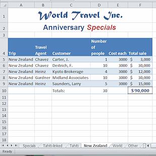
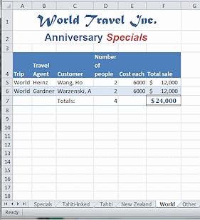
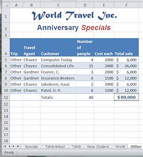
127 127

128 14. Switch to Page Layout View and create a header for all of the new sheets while they are still grouped - Name Date; File name - Sheet name; Excel Project Right click on a sheet tab and select Ungroup sheets! NEVER leave sheets grouped after you have finished working with the group. The next time you open the workbook those sheets will still be grouped... but you probably won't notice. Major opportunity for disaster!! 16. Save. [trips20-firstname-lastname.xlsx] Print: Entire Workbook Pay careful attention to what the Print dialog shows you are about to print. If sheets are grouped, they are all active sheets. The default choice for printing is to print All active sheet. 128

129 1. Print > Print > Entire workbook. Office button > File tab > Print > change Print Active Sheets to Print Entire Workbook 2. Look at the Print Preview. There are 7 pages since each sheet will fit on one page- Specials, Tahitilinked (in Landscape orientation and showing formulas still), Tahiti, New Zealand, World, Other, Tickets Sold Chart. Do some sheets need more than one page to print? You can change which pages to print in addition to picking which sheets to print. Often a sheet takes several pages. Excel 2007: Clicking the Preview button in the Print dialog opens a preview that reflects all of your choices in the Print dialog. Excel 2010: Changing which pages to print does NOT change the preview. Changing the between Print Active Sheets, Print Entire Workbook, and Print Selection DOES change the preview. 3. Print...unless your instructor tells you differently. 4. Save and close the workbook. [trips20-firstname-lastname.xlsx 129

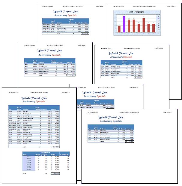
130 130