The goal is the definition of points with numbers and primitives with equations or functions. The definition of points with numbers requires a
|
|
|
- Chad Byrd
- 5 years ago
- Views:
Transcription
1
2 The goal is the definition of points with numbers and primitives with equations or functions. The definition of points with numbers requires a coordinate system and then the measuring of the point with respect to this coordinate system. A Cartesian coordinate system contains two orthogonal lines or axes, and a unit on them, and we measure how far we should walk along them to arrive at the identified point. A 2D polar coordinate system is a half line, and a point is defined by an angle and a distance. The angle specifies the direction in which we should go from the origin and the distance is interpreted between the origin and the identified point. Note that while we require that all points can be expressed by coordinates, this is not necessarily unambiguous, i.e. in a polar system the origin can be defined with arbitrary angle and with distance zero. In computer graphics barycentric coordinate systems are also popular. Here, the coordinate system is a set of points (at least 3 in 2D) where we put weights. The resulting mechanical system has a center of mass somewhere, which are identified by the numbers of the weights. Barycentric coordinates are often called homogeneous, due to the property that if we multiply all weights with the same non-zero scalar, then the center of mass is not affected. However, for such constructions we have already applied many non-trivial concepts like vectors, distance, angles. First, let us start from scratch and revisit these basic building
3 blocks.
4 If we want to specify 1D objects, like curves, then we should simultaneously identify (uncountably) infinitely many points. Obviously, defining the points one by one with their Cartesian coordinates is not an option. Instead, we usually specify an equation that has infinitely many roots and these roots are considered as the Cartesian coordinates of points in a set defined by the equation. Assume that we are in 2D when the equation should contain Cartesian coordinates x and y (in 3D there would be a third coordinate as well). The most obvious, but the least useful equation type is the explicit form, where we express y as a function of x. The problem with this representation is for each x there must be exactly one y. This is usually not the case, think of a circle or a vertical line, for example.
5 The equation can have implicit form, which means that x and y are put into an algebraic expression that is made equal to zero. We have a single equation with two unknowns thus, we have the hope of having infinitely many roots, i.e. x,y pairs. For example, a linear equation containing x and y identifies a line. A circle contains points that are at distance R from the reference point. Expressing this distance with the Pythagoras theorem, we can also develop and equation for the circle.
6 The equation may also have parametric form, where we use a free parameter t that can run in an appropriate interval. Substituting t into two equations defining x and y (or z), we get the Cartesian coordinates of the point corresponding to t.

7 For classic curves, like line, circle, parabola, ellipse, etc. we know their geometric definition, which can be translated to an equation, so the definition means the specification of the free parameters in the equation. However, curves we meet usually do not belong to the category of classic curves, so we do not know their equation. These curves are free form curves. As everything can be approximated by polynomials, the unknown equations of free form curves are also attacked this way. We approximate their parametric equations with polynomials of parameter t. The problem is that the polynomial coefficients do not have intuitive interpretation, thus we cannot expect the modeler to specify the coefficients directly. Instead, we require the user to specify a finite number of control points, and the modeling program automatically computes the polynomial coefficients from the control points. This computation can be an interpolation when the resulting curve is expected to go through the control points. Or, the computation can also be an approximation, when the resulting curve should just somehow follow the control points, but it does not have to go through each of them. By requiring approximation instead of interpolation, we ease the fitting process so we can impose additional requirements concerning the quality of the curve.
8 The first curve is of interpolation type and is known as the Lagrange interpolation. Suppose we specify a sequence of control points r1,, rn, and search a parametric function r(t) (one polynomial for each of the x, y or x, y, z coordinates) that goes through them. More precisely, we expect the curve to give control point r1 for parameter value t1, r2 for t2, etc. The interpolation requirement means n constraints, thus the polynomials may have n unknown coefficients to make the number of unknowns equal to the number of equations, and thus obtaining a well defined problem with an unambiguous solution. To find the n unknown polynomial coefficients, we need to solve a linear equation generated by substituting t1,,tn into the polynomial and requiring them to be equal to r1,,rn, respectively. If we solve it, we obtain the coefficients, which allow the computation of the curve point for arbitrary parameter t. Instead of solving the linear equation, the solution can be given directly as a combination of the control points with barycentric coordinates Li(t) that depend on parameter t. The algebraic form of these weight functions, aka basis functions or blending functions is shown here as the ratio of two products. To prove that the combination of the control points with these functions satisfies the interpolation constraints, let us examine a basis function Li when we substitute tk into it. If i=k, the numerator and the denominator of Li will be similar, so Li(ti) = 1. However, when i!=k, there will be some j which equals to k, so one factor of the numerator will be tk-tk=0, making Li(tk) also zero. So Li is 1 for ti but is zero for all other discrete parameter values. This means that in sum Li(tk) ri, all control points ri get zero weight except rk, which gets weight 1, thus r(tk) = rk. Note: A point of the Lagrange curve is the combination of control points with weights Li. According to the definition of combination, the reference points (which are the control points here) should be multiplied with the corresponding weights, the terms should be added them up, and finally the sum be divided with the total mass. Where is this division? The division can be ignored if the total mass is 1. Is the sum of the weight functions equal to 1 for any t??? (Yes).
9
10 Let us take an example where there are four control points and we expect the curve to interpolate them for t=0, 0.33, 0.67, and 1, respectively. The basis functions are depicted in the Figure. When t=0, the weight of the green point is 1, and the weight of all other points is zero. The curve is then in the green point. When t increases, the weight of the red point gets larger and at t=0.33 only the red point has non-zero weight The basis functions oscillate between positive and negative values, thus a control point periodically attracts or repels the curve. This is bad since the curve will tend to oscillate. The other disadvantage of Lagrange interpolation is that it cannot provide local control. Local control would mean that the modification of a control point modifies only a smaller part of the curve. However, as all basis functions are non-zero in the whole domain, the complete curve will change.
11 Hermite (H at the beginning and e at the end are silent because he was a Frenchman) interpolation is a generalization of Lagrange interpolation, where not only the points to be interpolated are given but also the derivatives. Here we discuss only the practically relevant special case, when the curve is defined by two control points and the first derivatives at these control points. We have four constraints, so the polynomial that is unambiguously determined by these constraints if a cubic (of four polynomical coefficients). The strategy is (always) similar to that of the Lagrange interpolation. We take the polynomial with yet unknown coefficients, substitute the constraints, and get a linear equation for the unknown coefficients. This linear equation is solved.
12 Lagrange (and Hermite) interpolation tends to oscillate. Let us find a better curve. We still use the center of mass analogy, i.e. the curve will be the composition of control points with weights placed at them. The weights are basis functions Bi(t) and we can ignore division with the total mass if the sum of weights is guaranteed to be equal to 1. We do not want the oscillation of the Lagrange curve, so we allow only nonnegative weights. Composition with non-negative weights is a convex combination, thus all points of the curve, i.e. the complete curve will be in the convex hull of the control points.
13 So, the task is to find a basis function system where each basis function is non-negative in the allowed domain (in [0,1]) and their sum is everywhere 1. Such basis functions can be constructed by expressing 1 with the Newtonian binomial theorem. The terms are called Bernstein polynomials, which are indeed non-negative if t is in [0,1], and their creation guarantees that their sum is 1.
14 If n = 3 (which is good for 4 control points), the basis functions are (1-t)^3, 3*(1-t)^2*t, 3*(1-t) *t^2, t^3. Note that the first basis function is 1 for t=0, while all others are zero, so the curve crosses the fist control points. Similarly, when t=1, the curve is at the last control point. However, other control points are not so lucky, they are usually not interpolated. This is an approximation curve.
15
16 Let us define a separate curve segments between every two control points applying Hermite interpolation. Hermite interpolation needs the start and end points (which are available) and the derivatives at these two points (which should be found somehow). If the speed is uniform and the motion is linear in segment i, then its constant speed equals to (r{i}-r{i-1})/(t{i}-t{i-1}). Similarly the constant speed in segment i+1 would be (r{i+1}-r{i})/(t{i+1}- t{i}). A good approximation is to set the velocity at the control point shared by the two segments to the average of these two velocities. This is the Catmull-Rom spline. Kochanek and Bartels further generalized this spline and allowed an additional tension parameter that can scale up or down the average velocity. On the other hand, we can use a weighted average when the average of the two constant speeds is obtained.

17
18
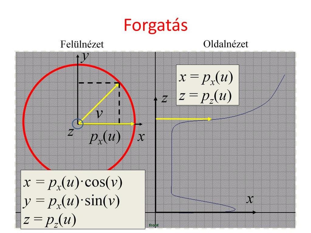
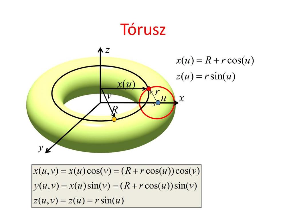
19 Surfaces are two dimensional subsets of the 3D space. Their definition is very similar to that of curves, but now the parametric equations have two free parameters (parametric equations of curves map a line segment onto the curve, parametric equations of surfaces map a square onto the surface).

20

21
22

23
24
25
26 The definition of curves traced back the problem to the specification of a few control points. We use the same approach here. First, we trace back the definition of surfaces to curves. Let us fix one of the free variables of the surface, which results in a one-variable parametric form, a curve. This curve is on the surface and is called isoparametric curve. A curve can be well defined by control points. Now let us fix the isoparametric value differently, which leads to another isoparametric curve that can be defined with different control points. As the isoparametric value changes, the control points of the corresponding isoparametric curve also change. These changes are also curves, so we can express the path of the control point by blending other control points. Substituting this into the equation of the isoparametric curve, we obtain the equation of the surface, which is a combination of control points forming a control cage or control polyhedron. The blending or weighting function of control point rij is the product of basis functions Bi parameterized with u, and Bj parameterized with v.

27 Surface definition is basically the modification of control points that attract the surface if weights are non-negative.

28 So far we used the following strategy. We started with the control cage or control mesh. Using the center of mass analogy, a continuous and smooth parametric surface is developed. However, when we render this smooth surface, we should decompose it to small triangles since the GPU can handle only triangles and not smooth surfaces. So the very beginning of this process is a rough mesh and the very end is a fine mesh. Can we get rid of the complicated mathematics of blending, splines, smooth interpolation etc. and obtain the fine mesh directly from the rough mesh?
29 Subdivision curves or surfaces are based exactly on this idea. Let us consider a curve defined by a few control points. The polyline connecting the control points is a rough approximation of the desired smooth curve. This rough polyline is refined by subdividing it by inserting a point at the middle of each line segment and then moving the original vertices to the weighted average of their original location and the two middle points. The new polyline looks smoother. If we are not satisfied, we can repeat the process recursively.

30 The idea can be extended to surfaces. Here only one type of subdivision surfaces is introduced, which is called the Catmull-Clark surface. We assume that the original mesh is built of quadrilaterals. Although the algorithm can work with other meshes as well, after the first subdivision step, the mesh will always be a quadrilateral mesh. The subdivision starts by the computation of face center and edge center points, which double the resolution but do not alter the shape yet. Then we first move the original vertices to the weighted average of the surrounding face centers, edge centers and of the point itself. The averaging scheme also depends on how many faces share this point, which is called the valence of this vertex. Having moved the original vertices, we find the final location of the edge centers as well.
31
32
33
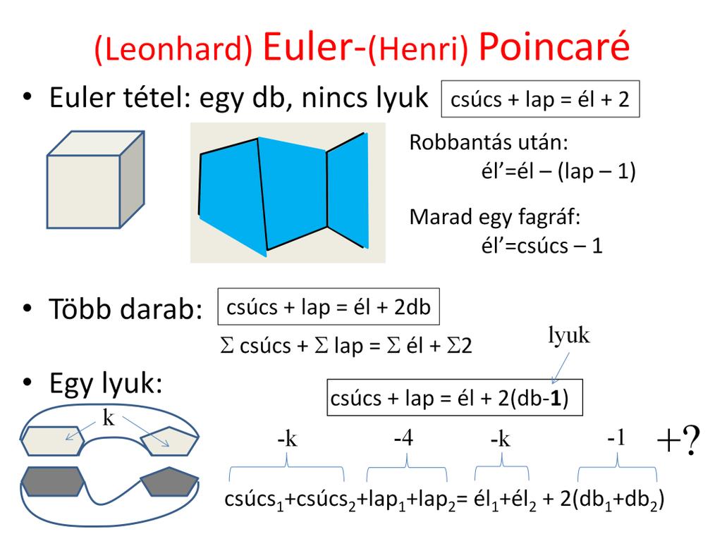
34 Boundary representation defines a solid by the boundary surfaces or faces. Specifying the boundaries independently would not work since it would be possible to create something where the boundaries do not enclose a 3D solid or the enclosing is not watertight. We should specify edges, faces and vertices simultaneously to always guarantee that the object is topologically valid. A famous equation that can be used to check topological validity is the Euler theorem. It can be applied for 3D objects that are isomorphic to a sphere (they turn to a sphere when pumped up). Objects with holes or consisting of multiple independent pieces do not belong this category (they are isomorphic to a torus or more than one sphere). The Euler equation can be generalized to cover these cases as well, when it is called Euler- Poincare equation. With the Euler s theorem, when we have an object, counting the vertices, faces and edges allows the determination whether or not this object is valid. However, when it turns out that it is invalid, it is usually too late. What we need is elementary operations that keep the validity of the Euler equation provided it was valid before the application of the operation. Such elementary operations are called Euler operations.
35
, edges (8) and vertices (8), we can prove that it is indeed an Euler operator.")
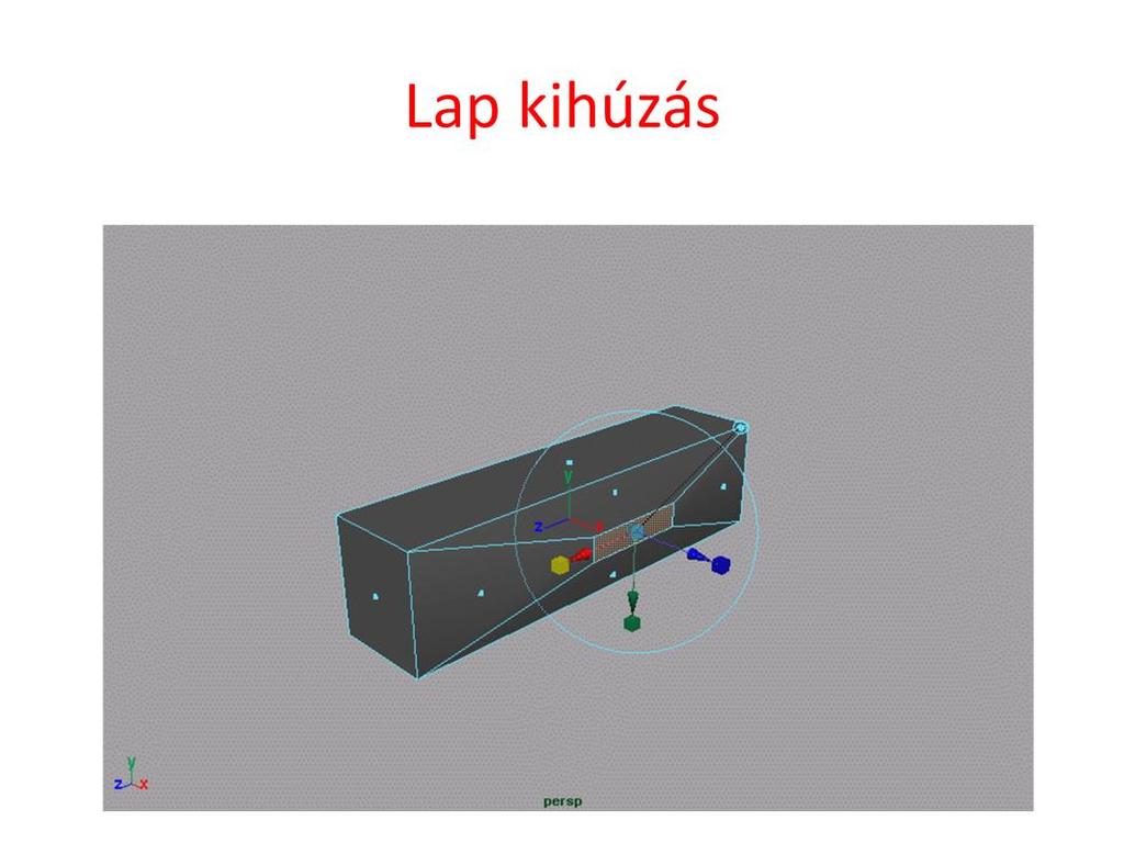
36 A few examples of Euler operators are shown here. Face extrude extrudes a face by automatically filling the holes between the original and extruded face with new faces and edges. Counting the numbers of new faces (4), edges (8) and vertices (8), we can prove that it is indeed an Euler operator. Face split requires the user to select two edges of a fact and to specify two points on them. These new points are connected by a new edge. Altogether, this operation introduces 2 vertices, 3 edges (one new and two that are obtained as the subdivision of the original edges with the new points) and a new face (the new edge subdivides the face into two). Edge collapse removes an edge with one of its end points. Vertex split is the inverse of this operation.
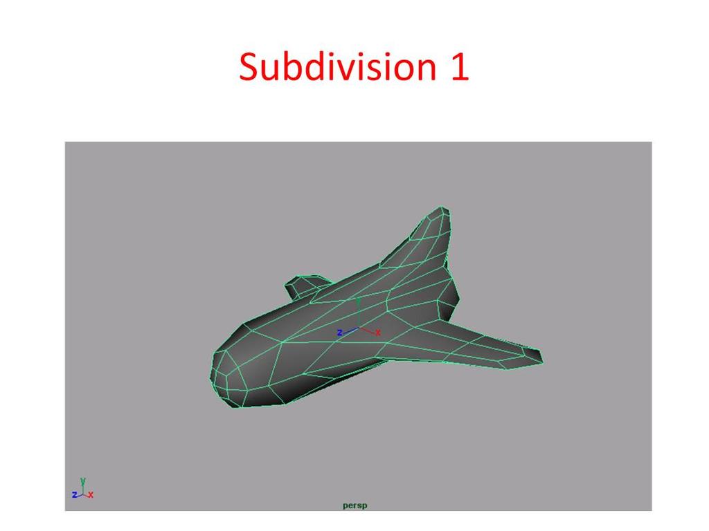
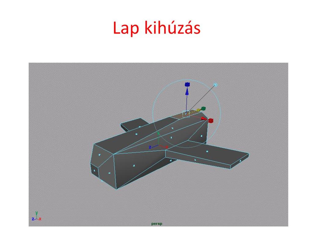
37 To create a space ship, we can start with a topologically valid object, e.g. a transformed cube, then we execute a sequence of face extrusions. As face extrude is an Euler operator, the result will automatically be a topologically valid object.
38
39
40

41
42
43
08 - Designing Approximating Curves
 08 - Designing Approximating Curves Acknowledgement: Olga Sorkine-Hornung, Alexander Sorkine-Hornung, Ilya Baran Last time Interpolating curves Monomials Lagrange Hermite Different control types Polynomials
From curves to surfaces. Parametric surfaces and solid modeling. Extrusions. Surfaces of revolution. So far have discussed spline curves in 2D
 From curves to surfaces Parametric surfaces and solid modeling CS 465 Lecture 12 2007 Doug James & Steve Marschner 1 So far have discussed spline curves in 2D it turns out that this already provides of
Fall CSCI 420: Computer Graphics. 4.2 Splines. Hao Li.
 Fall 2014 CSCI 420: Computer Graphics 4.2 Splines Hao Li http://cs420.hao-li.com 1 Roller coaster Next programming assignment involves creating a 3D roller coaster animation We must model the 3D curve
Splines. Parameterization of a Curve. Curve Representations. Roller coaster. What Do We Need From Curves in Computer Graphics? Modeling Complex Shapes
 CSCI 420 Computer Graphics Lecture 8 Splines Jernej Barbic University of Southern California Hermite Splines Bezier Splines Catmull-Rom Splines Other Cubic Splines [Angel Ch 12.4-12.12] Roller coaster
Parametric curves. Brian Curless CSE 457 Spring 2016
 Parametric curves Brian Curless CSE 457 Spring 2016 1 Reading Required: Angel 10.1-10.3, 10.5.2, 10.6-10.7, 10.9 Optional Bartels, Beatty, and Barsky. An Introduction to Splines for use in Computer Graphics
Until now we have worked with flat entities such as lines and flat polygons. Fit well with graphics hardware Mathematically simple
 Curves and surfaces Escaping Flatland Until now we have worked with flat entities such as lines and flat polygons Fit well with graphics hardware Mathematically simple But the world is not composed of
Sung-Eui Yoon ( 윤성의 )
") CS480: Computer Graphics Curves and Surfaces Sung-Eui Yoon ( 윤성의 ) Course URL: http://jupiter.kaist.ac.kr/~sungeui/cg Today s Topics Surface representations Smooth curves Subdivision 2 Smooth Curves and
CS480: Computer Graphics Curves and Surfaces Sung-Eui Yoon ( 윤성의 ) Course URL: http://jupiter.kaist.ac.kr/~sungeui/cg Today s Topics Surface representations Smooth curves Subdivision 2 Smooth Curves and
Design considerations
 Curves Design considerations local control of shape design each segment independently smoothness and continuity ability to evaluate derivatives stability small change in input leads to small change in
Know it. Control points. B Spline surfaces. Implicit surfaces
 Know it 15 B Spline Cur 14 13 12 11 Parametric curves Catmull clark subdivision Parametric surfaces Interpolating curves 10 9 8 7 6 5 4 3 2 Control points B Spline surfaces Implicit surfaces Bezier surfaces
CS354 Computer Graphics Surface Representation IV. Qixing Huang March 7th 2018
 CS354 Computer Graphics Surface Representation IV Qixing Huang March 7th 2018 Today s Topic Subdivision surfaces Implicit surface representation Subdivision Surfaces Building complex models We can extend
Surfaces for CAGD. FSP Tutorial. FSP-Seminar, Graz, November
 Surfaces for CAGD FSP Tutorial FSP-Seminar, Graz, November 2005 1 Tensor Product Surfaces Given: two curve schemes (Bézier curves or B splines): I: x(u) = m i=0 F i(u)b i, u [a, b], II: x(v) = n j=0 G
2D Spline Curves. CS 4620 Lecture 13
 2D Spline Curves CS 4620 Lecture 13 2008 Steve Marschner 1 Motivation: smoothness In many applications we need smooth shapes [Boeing] that is, without discontinuities So far we can make things with corners
Curve Representation ME761A Instructor in Charge Prof. J. Ramkumar Department of Mechanical Engineering, IIT Kanpur
 Curve Representation ME761A Instructor in Charge Prof. J. Ramkumar Department of Mechanical Engineering, IIT Kanpur Email: jrkumar@iitk.ac.in Curve representation 1. Wireframe models There are three types
Lecture IV Bézier Curves
 Lecture IV Bézier Curves Why Curves? Why Curves? Why Curves? Why Curves? Why Curves? Linear (flat) Curved Easier More pieces Looks ugly Complicated Fewer pieces Looks smooth What is a curve? Intuitively:
Parametric Curves. University of Texas at Austin CS384G - Computer Graphics Fall 2010 Don Fussell
 Parametric Curves University of Texas at Austin CS384G - Computer Graphics Fall 2010 Don Fussell Parametric Representations 3 basic representation strategies: Explicit: y = mx + b Implicit: ax + by + c
Information Coding / Computer Graphics, ISY, LiTH. Splines
 28(69) Splines Originally a drafting tool to create a smooth curve In computer graphics: a curve built from sections, each described by a 2nd or 3rd degree polynomial. Very common in non-real-time graphics,
Central issues in modelling
 Central issues in modelling Construct families of curves, surfaces and volumes that can represent common objects usefully; are easy to interact with; interaction includes: manual modelling; fitting to
Parametric curves. Reading. Curves before computers. Mathematical curve representation. CSE 457 Winter Required:
 Reading Required: Angel 10.1-10.3, 10.5.2, 10.6-10.7, 10.9 Parametric curves CSE 457 Winter 2014 Optional Bartels, Beatty, and Barsky. An Introduction to Splines for use in Computer Graphics and Geometric
2D rendering takes a photo of the 2D scene with a virtual camera that selects an axis aligned rectangle from the scene. The photograph is placed into
 2D rendering takes a photo of the 2D scene with a virtual camera that selects an axis aligned rectangle from the scene. The photograph is placed into the viewport of the current application window. A pixel
ECE 600, Dr. Farag, Summer 09
 ECE 6 Summer29 Course Supplements. Lecture 4 Curves and Surfaces Aly A. Farag University of Louisville Acknowledgements: Help with these slides were provided by Shireen Elhabian A smile is a curve that
Geometric transformations assign a point to a point, so it is a point valued function of points. Geometric transformation may destroy the equation
 Geometric transformations assign a point to a point, so it is a point valued function of points. Geometric transformation may destroy the equation and the type of an object. Even simple scaling turns a
Parametric Curves. University of Texas at Austin CS384G - Computer Graphics
 Parametric Curves University of Texas at Austin CS384G - Computer Graphics Fall 2010 Don Fussell Parametric Representations 3 basic representation strategies: Explicit: y = mx + b Implicit: ax + by + c
Representing Curves Part II. Foley & Van Dam, Chapter 11
 Representing Curves Part II Foley & Van Dam, Chapter 11 Representing Curves Polynomial Splines Bezier Curves Cardinal Splines Uniform, non rational B-Splines Drawing Curves Applications of Bezier splines
Curves D.A. Forsyth, with slides from John Hart
 Curves D.A. Forsyth, with slides from John Hart Central issues in modelling Construct families of curves, surfaces and volumes that can represent common objects usefully; are easy to interact with; interaction
2D Spline Curves. CS 4620 Lecture 18
 2D Spline Curves CS 4620 Lecture 18 2014 Steve Marschner 1 Motivation: smoothness In many applications we need smooth shapes that is, without discontinuities So far we can make things with corners (lines,
COMPUTER AIDED ENGINEERING DESIGN (BFF2612)
") COMPUTER AIDED ENGINEERING DESIGN (BFF2612) BASIC MATHEMATICAL CONCEPTS IN CAED by Dr. Mohd Nizar Mhd Razali Faculty of Manufacturing Engineering mnizar@ump.edu.my COORDINATE SYSTEM y+ y+ z+ z+ x+ RIGHT
COMPUTER AIDED ENGINEERING DESIGN (BFF2612) BASIC MATHEMATICAL CONCEPTS IN CAED by Dr. Mohd Nizar Mhd Razali Faculty of Manufacturing Engineering mnizar@ump.edu.my COORDINATE SYSTEM y+ y+ z+ z+ x+ RIGHT
OUTLINE. Quadratic Bezier Curves Cubic Bezier Curves
 BEZIER CURVES 1 OUTLINE Introduce types of curves and surfaces Introduce the types of curves Interpolating Hermite Bezier B-spline Quadratic Bezier Curves Cubic Bezier Curves 2 ESCAPING FLATLAND Until
Curves and Surfaces. Shireen Elhabian and Aly A. Farag University of Louisville
 Curves and Surfaces Shireen Elhabian and Aly A. Farag University of Louisville February 21 A smile is a curve that sets everything straight Phyllis Diller (American comedienne and actress, born 1917) Outline
Lecture 2.2 Cubic Splines
 Lecture. Cubic Splines Cubic Spline The equation for a single parametric cubic spline segment is given by 4 i t Bit t t t i (..) where t and t are the parameter values at the beginning and end of the segment.
3D Modeling Parametric Curves & Surfaces. Shandong University Spring 2013
 3D Modeling Parametric Curves & Surfaces Shandong University Spring 2013 3D Object Representations Raw data Point cloud Range image Polygon soup Surfaces Mesh Subdivision Parametric Implicit Solids Voxels
Introduction to Computer Graphics
 Introduction to Computer Graphics 2016 Spring National Cheng Kung University Instructors: Min-Chun Hu 胡敏君 Shih-Chin Weng 翁士欽 ( 西基電腦動畫 ) Data Representation Curves and Surfaces Limitations of Polygons Inherently
Computer Graphics Curves and Surfaces. Matthias Teschner
 Computer Graphics Curves and Surfaces Matthias Teschner Outline Introduction Polynomial curves Bézier curves Matrix notation Curve subdivision Differential curve properties Piecewise polynomial curves
Intro to Curves Week 1, Lecture 2
 CS 536 Computer Graphics Intro to Curves Week 1, Lecture 2 David Breen, William Regli and Maxim Peysakhov Department of Computer Science Drexel University Outline Math review Introduction to 2D curves
The Free-form Surface Modelling System
 1. Introduction The Free-form Surface Modelling System Smooth curves and surfaces must be generated in many computer graphics applications. Many real-world objects are inherently smooth (fig.1), and much
3D Modeling Parametric Curves & Surfaces
 3D Modeling Parametric Curves & Surfaces Shandong University Spring 2012 3D Object Representations Raw data Point cloud Range image Polygon soup Solids Voxels BSP tree CSG Sweep Surfaces Mesh Subdivision
CS 536 Computer Graphics Intro to Curves Week 1, Lecture 2
 CS 536 Computer Graphics Intro to Curves Week 1, Lecture 2 David Breen, William Regli and Maxim Peysakhov Department of Computer Science Drexel University 1 Outline Math review Introduction to 2D curves
Physically-Based Modeling and Animation. University of Missouri at Columbia
 Overview of Geometric Modeling Overview 3D Shape Primitives: Points Vertices. Curves Lines, polylines, curves. Surfaces Triangle meshes, splines, subdivision surfaces, implicit surfaces, particles. Solids
09 - Designing Surfaces. CSCI-GA Computer Graphics - Fall 16 - Daniele Panozzo
 9 - Designing Surfaces Triangular surfaces A surface can be discretized by a collection of points and triangles Each triangle is a subset of a plane Every point on the surface can be expressed as an affine
Computergrafik. Matthias Zwicker. Herbst 2010
 Computergrafik Matthias Zwicker Universität Bern Herbst 2010 Today Curves NURBS Surfaces Parametric surfaces Bilinear patch Bicubic Bézier patch Advanced surface modeling Piecewise Bézier curves Each segment
Computergrafik. Matthias Zwicker Universität Bern Herbst 2016
 Computergrafik Matthias Zwicker Universität Bern Herbst 2016 Today Curves NURBS Surfaces Parametric surfaces Bilinear patch Bicubic Bézier patch Advanced surface modeling 2 Piecewise Bézier curves Each
Curves and Surfaces Computer Graphics I Lecture 10
 15-462 Computer Graphics I Lecture 10 Curves and Surfaces Parametric Representations Cubic Polynomial Forms Hermite Curves Bezier Curves and Surfaces [Angel 10.1-10.6] September 30, 2003 Doug James Carnegie
Barycentric Coordinates and Parameterization
 Barycentric Coordinates and Parameterization Center of Mass Geometric center of object Center of Mass Geometric center of object Object can be balanced on CoM How to calculate? Finding the Center of Mass
Intro to Modeling Modeling in 3D
 Intro to Modeling Modeling in 3D Polygon sets can approximate more complex shapes as discretized surfaces 2 1 2 3 Curve surfaces in 3D Sphere, ellipsoids, etc Curved Surfaces Modeling in 3D ) ( 2 2 2 2
Curve and Surface Basics
 Curve and Surface Basics Implicit and parametric forms Power basis form Bezier curves Rational Bezier Curves Tensor Product Surfaces ME525x NURBS Curve and Surface Modeling Page 1 Implicit and Parametric
Curves and Surfaces Computer Graphics I Lecture 9
 15-462 Computer Graphics I Lecture 9 Curves and Surfaces Parametric Representations Cubic Polynomial Forms Hermite Curves Bezier Curves and Surfaces [Angel 10.1-10.6] February 19, 2002 Frank Pfenning Carnegie
An introduction to interpolation and splines
 An introduction to interpolation and splines Kenneth H. Carpenter, EECE KSU November 22, 1999 revised November 20, 2001, April 24, 2002, April 14, 2004 1 Introduction Suppose one wishes to draw a curve
Lecture 25: Bezier Subdivision. And he took unto him all these, and divided them in the midst, and laid each piece one against another: Genesis 15:10
 Lecture 25: Bezier Subdivision And he took unto him all these, and divided them in the midst, and laid each piece one against another: Genesis 15:10 1. Divide and Conquer If we are going to build useful
Computer Graphics CS 543 Lecture 13a Curves, Tesselation/Geometry Shaders & Level of Detail
 Computer Graphics CS 54 Lecture 1a Curves, Tesselation/Geometry Shaders & Level of Detail Prof Emmanuel Agu Computer Science Dept. Worcester Polytechnic Institute (WPI) So Far Dealt with straight lines
Interactive Graphics. Lecture 9: Introduction to Spline Curves. Interactive Graphics Lecture 9: Slide 1
 Interactive Graphics Lecture 9: Introduction to Spline Curves Interactive Graphics Lecture 9: Slide 1 Interactive Graphics Lecture 13: Slide 2 Splines The word spline comes from the ship building trade
Outline. Visualization Discretization Sampling Quantization Representation Continuous Discrete. Noise
 Fundamentals Data Outline Visualization Discretization Sampling Quantization Representation Continuous Discrete Noise 2 Data Data : Function dependent on one or more variables. Example Audio (1D) - depends
Honors Precalculus: Solving equations and inequalities graphically and algebraically. Page 1
 Solving equations and inequalities graphically and algebraically 1. Plot points on the Cartesian coordinate plane. P.1 2. Represent data graphically using scatter plots, bar graphs, & line graphs. P.1
Bezier Curves, B-Splines, NURBS
 Bezier Curves, B-Splines, NURBS Example Application: Font Design and Display Curved objects are everywhere There is always need for: mathematical fidelity high precision artistic freedom and flexibility
Objects 2: Curves & Splines Christian Miller CS Fall 2011
 Objects 2: Curves & Splines Christian Miller CS 354 - Fall 2011 Parametric curves Curves that are defined by an equation and a parameter t Usually t [0, 1], and curve is finite Can be discretized at arbitrary
GEOMETRIC TOOLS FOR COMPUTER GRAPHICS
 GEOMETRIC TOOLS FOR COMPUTER GRAPHICS PHILIP J. SCHNEIDER DAVID H. EBERLY MORGAN KAUFMANN PUBLISHERS A N I M P R I N T O F E L S E V I E R S C I E N C E A M S T E R D A M B O S T O N L O N D O N N E W
Splines. Connecting the Dots
 Splines or: Connecting the Dots Jens Ogniewski Information Coding Group Linköping University Before we start... Some parts won t be part of the exam Basically all that is not described in the book. More
Mathematics Background
 Finding Area and Distance Students work in this Unit develops a fundamentally important relationship connecting geometry and algebra: the Pythagorean Theorem. The presentation of ideas in the Unit reflects
GL9: Engineering Communications. GL9: CAD techniques. Curves Surfaces Solids Techniques
 436-105 Engineering Communications GL9:1 GL9: CAD techniques Curves Surfaces Solids Techniques Parametric curves GL9:2 x = a 1 + b 1 u + c 1 u 2 + d 1 u 3 + y = a 2 + b 2 u + c 2 u 2 + d 2 u 3 + z = a
Voluntary State Curriculum Algebra II
 Algebra II Goal 1: Integration into Broader Knowledge The student will develop, analyze, communicate, and apply models to real-world situations using the language of mathematics and appropriate technology.
Curves and Surfaces 2
 Curves and Surfaces 2 Computer Graphics Lecture 17 Taku Komura Today More about Bezier and Bsplines de Casteljau s algorithm BSpline : General form de Boor s algorithm Knot insertion NURBS Subdivision
Lecture 17: Solid Modeling.... a cubit on the one side, and a cubit on the other side Exodus 26:13
 Lecture 17: Solid Modeling... a cubit on the one side, and a cubit on the other side Exodus 26:13 Who is on the LORD's side? Exodus 32:26 1. Solid Representations A solid is a 3-dimensional shape with
3D Modeling techniques
 3D Modeling techniques 0. Reconstruction From real data (not covered) 1. Procedural modeling Automatic modeling of a self-similar objects or scenes 2. Interactive modeling Provide tools to computer artists
Mathematical Tools in Computer Graphics with C# Implementations Table of Contents
 Mathematical Tools in Computer Graphics with C# Implementations by Hardy Alexandre, Willi-Hans Steeb, World Scientific Publishing Company, Incorporated, 2008 Table of Contents List of Figures Notation
Advanced Operations Research Techniques IE316. Quiz 1 Review. Dr. Ted Ralphs
 Advanced Operations Research Techniques IE316 Quiz 1 Review Dr. Ted Ralphs IE316 Quiz 1 Review 1 Reading for The Quiz Material covered in detail in lecture. 1.1, 1.4, 2.1-2.6, 3.1-3.3, 3.5 Background material
Shape modeling Modeling technique Shape representation! 3D Graphics Modeling Techniques
 D Graphics http://chamilo2.grenet.fr/inp/courses/ensimag4mmgd6/ Shape Modeling technique Shape representation! Part : Basic techniques. Projective rendering pipeline 2. Procedural Modeling techniques Shape
Introduction p. 1 What Is Geometric Modeling? p. 1 Computer-aided geometric design Solid modeling Algebraic geometry Computational geometry
 Introduction p. 1 What Is Geometric Modeling? p. 1 Computer-aided geometric design Solid modeling Algebraic geometry Computational geometry Representation Ab initio design Rendering Solid modelers Kinematic
Curves, Surfaces and Recursive Subdivision
 Department of Computer Sciences Graphics Fall 25 (Lecture ) Curves, Surfaces and Recursive Subdivision Conics: Curves and Quadrics: Surfaces Implicit form arametric form Rational Bézier Forms Recursive
B-spline Curves. Smoother than other curve forms
 Curves and Surfaces B-spline Curves These curves are approximating rather than interpolating curves. The curves come close to, but may not actually pass through, the control points. Usually used as multiple,
CS 450 Numerical Analysis. Chapter 7: Interpolation
 Lecture slides based on the textbook Scientific Computing: An Introductory Survey by Michael T. Heath, copyright c 2018 by the Society for Industrial and Applied Mathematics. http://www.siam.org/books/cl80
u 0+u 2 new boundary vertex
 Combined Subdivision Schemes for the design of surfaces satisfying boundary conditions Adi Levin School of Mathematical Sciences, Tel-Aviv University, Tel-Aviv 69978, Israel. Email:fadilev@math.tau.ac.ilg
Interactive Computer Graphics A TOP-DOWN APPROACH WITH SHADER-BASED OPENGL
 International Edition Interactive Computer Graphics A TOP-DOWN APPROACH WITH SHADER-BASED OPENGL Sixth Edition Edward Angel Dave Shreiner Interactive Computer Graphics: A Top-Down Approach with Shader-Based
Joe Warren, Scott Schaefer Rice University
 Joe Warren, Scott Schaefer Rice University Polygons are a ubiquitous modeling primitive in computer graphics. Their popularity is such that special purpose graphics hardware designed to render polygons
Solid Modeling. Ron Goldman Department of Computer Science Rice University
 Solid Modeling Ron Goldman Department of Computer Science Rice University Solids Definition 1. A model which has a well defined inside and outside. 2. For each point, we can in principle determine whether
Dgp _ lecture 2. Curves
 Dgp _ lecture 2 Curves Questions? This lecture will be asking questions about curves, their Relationship to surfaces, and how they are used and controlled. Topics of discussion will be: Free form Curves
Cecil Jones Academy Mathematics Fundamentals
 Year 10 Fundamentals Core Knowledge Unit 1 Unit 2 Estimate with powers and roots Calculate with powers and roots Explore the impact of rounding Investigate similar triangles Explore trigonometry in right-angled
Shape Representation Basic problem We make pictures of things How do we describe those things? Many of those things are shapes Other things include
 Shape Representation Basic problem We make pictures of things How do we describe those things? Many of those things are shapes Other things include motion, behavior Graphics is a form of simulation and
CS123 INTRODUCTION TO COMPUTER GRAPHICS. Describing Shapes. Constructing Objects in Computer Graphics 1/15
 Describing Shapes Constructing Objects in Computer Graphics 1/15 2D Object Definition (1/3) Lines and polylines: Polylines: lines drawn between ordered points A closed polyline is a polygon, a simple polygon
COMPUTER AIDED GEOMETRIC DESIGN. Thomas W. Sederberg
 COMPUTER AIDED GEOMETRIC DESIGN Thomas W. Sederberg January 31, 2011 ii T. W. Sederberg iii Preface This semester is the 24 th time I have taught a course at Brigham Young University titled, Computer Aided
INF3320 Computer Graphics and Discrete Geometry
 INF3320 Computer Graphics and Discrete Geometry More smooth Curves and Surfaces Christopher Dyken, Michael Floater and Martin Reimers 10.11.2010 Page 1 More smooth Curves and Surfaces Akenine-Möller, Haines
CS-184: Computer Graphics
 CS-184: Computer Graphics Lecture #12: Curves and Surfaces Prof. James O Brien University of California, Berkeley V2007-F-12-1.0 Today General curve and surface representations Splines and other polynomial
Parameterization of triangular meshes
 Parameterization of triangular meshes Michael S. Floater November 10, 2009 Triangular meshes are often used to represent surfaces, at least initially, one reason being that meshes are relatively easy to
Subdivision Surfaces
 Subdivision Surfaces 1 Geometric Modeling Sometimes need more than polygon meshes Smooth surfaces Traditional geometric modeling used NURBS Non uniform rational B-Spline Demo 2 Problems with NURBS A single
A Curve Tutorial for Introductory Computer Graphics
 A Curve Tutorial for Introductory Computer Graphics Michael Gleicher Department of Computer Sciences University of Wisconsin, Madison October 7, 2003 Note to 559 Students: These notes were put together
CHAPTER 1 Graphics Systems and Models 3
 ?????? 1 CHAPTER 1 Graphics Systems and Models 3 1.1 Applications of Computer Graphics 4 1.1.1 Display of Information............. 4 1.1.2 Design.................... 5 1.1.3 Simulation and Animation...........
Subdivision Surfaces
 Subdivision Surfaces 1 Geometric Modeling Sometimes need more than polygon meshes Smooth surfaces Traditional geometric modeling used NURBS Non uniform rational B-Spline Demo 2 Problems with NURBS A single
Geometric Modeling of Curves
 Curves Locus of a point moving with one degree of freedom Locus of a one-dimensional parameter family of point Mathematically defined using: Explicit equations Implicit equations Parametric equations (Hermite,
A Flavor of Topology. Shireen Elhabian and Aly A. Farag University of Louisville January 2010
 A Flavor of Topology Shireen Elhabian and Aly A. Farag University of Louisville January 2010 In 1670 s I believe that we need another analysis properly geometric or linear, which treats place directly
CS337 INTRODUCTION TO COMPUTER GRAPHICS. Describing Shapes. Constructing Objects in Computer Graphics. Bin Sheng Representing Shape 9/20/16 1/15
 Describing Shapes Constructing Objects in Computer Graphics 1/15 2D Object Definition (1/3) Lines and polylines: Polylines: lines drawn between ordered points A closed polyline is a polygon, a simple polygon
Curves and Surfaces 1
 Curves and Surfaces 1 Representation of Curves & Surfaces Polygon Meshes Parametric Cubic Curves Parametric Bi-Cubic Surfaces Quadric Surfaces Specialized Modeling Techniques 2 The Teapot 3 Representing
Intro to Curves Week 4, Lecture 7
 CS 430/536 Computer Graphics I Intro to Curves Week 4, Lecture 7 David Breen, William Regli and Maxim Peysakhov Geometric and Intelligent Computing Laboratory Department of Computer Science Drexel University
30. Constrained Optimization
 30. Constrained Optimization The graph of z = f(x, y) is represented by a surface in R 3. Normally, x and y are chosen independently of one another so that one may roam over the entire surface of f (within
Rendering Curves and Surfaces. Ed Angel Professor of Computer Science, Electrical and Computer Engineering, and Media Arts University of New Mexico
 Rendering Curves and Surfaces Ed Angel Professor of Computer Science, Electrical and Computer Engineering, and Media Arts University of New Mexico Objectives Introduce methods to draw curves - Approximate
Rendering Subdivision Surfaces Efficiently on the GPU
 Rendering Subdivision Surfaces Efficiently on the GPU Gy. Antal, L. Szirmay-Kalos and L. A. Jeni Department of Algorithms and their Applications, Faculty of Informatics, Eötvös Loránd Science University,
1.1 calculator viewing window find roots in your calculator 1.2 functions find domain and range (from a graph) may need to review interval notation
 may need to review interval notation") 1.1 calculator viewing window find roots in your calculator 1.2 functions find domain and range (from a graph) may need to review interval notation functions vertical line test function notation evaluate
1.1 calculator viewing window find roots in your calculator 1.2 functions find domain and range (from a graph) may need to review interval notation functions vertical line test function notation evaluate
Homework #2. Shading, Projections, Texture Mapping, Ray Tracing, and Bezier Curves
 Computer Graphics Instructor: Brian Curless CSEP 557 Autumn 2016 Homework #2 Shading, Projections, Texture Mapping, Ray Tracing, and Bezier Curves Assigned: Wednesday, Nov 16 th Due: Wednesday, Nov 30
CS130 : Computer Graphics Curves. Tamar Shinar Computer Science & Engineering UC Riverside
 CS130 : Computer Graphics Curves Tamar Shinar Computer Science & Engineering UC Riverside Design considerations local control of shape design each segment independently smoothness and continuity ability
Perspective Mappings. Contents
 Perspective Mappings David Eberly, Geometric Tools, Redmond WA 98052 https://www.geometrictools.com/ This work is licensed under the Creative Commons Attribution 4.0 International License. To view a copy
Grade 9 Math Terminology
 Unit 1 Basic Skills Review BEDMAS a way of remembering order of operations: Brackets, Exponents, Division, Multiplication, Addition, Subtraction Collect like terms gather all like terms and simplify as
A.1 Numbers, Sets and Arithmetic
 522 APPENDIX A. MATHEMATICS FOUNDATIONS A.1 Numbers, Sets and Arithmetic Numbers started as a conceptual way to quantify count objects. Later, numbers were used to measure quantities that were extensive,
Parameterization. Michael S. Floater. November 10, 2011
 Parameterization Michael S. Floater November 10, 2011 Triangular meshes are often used to represent surfaces, at least initially, one reason being that meshes are relatively easy to generate from point
Subdivision overview
 Subdivision overview CS4620 Lecture 16 2018 Steve Marschner 1 Introduction: corner cutting Piecewise linear curve too jagged for you? Lop off the corners! results in a curve with twice as many corners