Three-dimensional direct numerical simulation of wake transitions of a circular cylinder

Transcription

1 Three-dimensional direct numerical simulation of wake transitions of a circular cylinder HONGYI JIANG 1, LIANG CHENG 1,2, SCOTT DRAPER 1,3, HONGWEI AN 1 AND FEIFEI TONG 1 1 School of Civil, Environmental and Mining Engineering, The University of Western Australia, 35 Stirling Highway, Crawley, WA 6009, Australia 2 State Key Laboratory of Coastal and Offshore Engineering, Dalian University of Technology, Dalian, , China 3 Centre for Offshore Foundation Systems, The University of Western Australia, 35 Stirling Highway, Crawley, WA 6009, Australia Abstract This paper presents three-dimensional (3D) direct numerical simulations (DNS) of flow past a circular cylinder over a range of Reynolds number (Re) up to 300. The gradual wake transition process from Mode A* (i.e. Mode A with large-scale vortex dislocations) to Mode B is well captured over a range of Re from 230 to 260. The mode swapping process is investigated in detail with the aid of numerical flow visualization. It is found that the Mode B structures in the transition process are developed based on the streamwise vortices of Mode A or A* which destabilize the braid shear layer region. For each case within the transition range, the transient mode swapping process consists of dislocation and non-dislocation cycles. With the increase of Re, it becomes more difficult to trigger dislocations from the pure Mode A structure and form a dislocation cycle, and each dislocation stage becomes shorter in duration, resulting in a continuous decrease in the probability of occurrence of Mode A* and a continuous increase in the probability of occurrence of Mode B. The occurrence of Mode A* results in a relatively strong flow three-dimensionality. A critical condition is confirmed at approximately Re = where the weakest flow three-dimensionality is observed, marking a transition from the disappearance of address for correspondence: hongyijiang88@gmail.com 1

2 Mode A* to the emergence of increasingly disordered Mode B structures. 1. Introduction Steady incoming flow past a long circular cylinder at relatively low values of the Reynolds number (Re) has been the topic of extensive studies due to its fundamental and practical significance. It is well known that the flow is governed by a single dimensionless parameter Re, which is defined based on the approaching flow velocity U, the cylinder diameter D and the kinematic viscosity of the fluid ν. Methods of investigation have included physical model testing, direct numerical simulation (DNS) and linear (and non-linear) stability analysis. Comprehensive reviews on investigations of flow with different methodologies can be found, for example, in Williamson (1996a, 1996b) and Posdziech and Grundmann (2001). Based on these investigations, it has been shown (e.g. Williamson, 1996a) that for flow past a circular cylinder the flow structure in the wake will undergo a transition sequence of: (1) emergence of primary wake instability at Re ~ 47, (2) onset of Mode A instability with large-scale vortex dislocations (i.e. Mode A*) at Re ~ 190, (3) the gradual transition from Mode A* to Mode B over a range of Re from 230 to 250, and (4) development of increasingly disordered Mode B structure beyond Re = 260. Many previous studies have focused on identifying the critical Reynolds number Re cr at which Mode A* wake instability emerges. The Re cr values identified by some experimental studies are: 150 by Roshko (1954) and Tritton (1959), 165 by Norberg (1994), 178 by Williamson (1988, 1989), 194 by Williamson (1996b), and 205 by Miller and Williamson (1994). It was discovered that the low values of Re cr identified by early experimental studies were largely due to the end effect (Williamson, 1996b). Williamson (1996b) extended the Re cr value to 194 by eliminating end effects using non-mechanical end conditions. This value is very close to the Re cr values of (±1.0), (±0.02) and predicted through linear stability analysis by Barkley and Henderson (1996), Posdziech and Grundmann (2001), and Rao et al. (2013), respectively. 2

3 According to the experimental study by Williamson (1996b), Mode B wake instability first emerges at Re ~ 230, which is much lower than the critical Re of 259 and 261 (±0.2) for Mode B instability predicted through linear stability analysis by Barkley and Henderson (1996) and Posdziech and Grundmann (2001), respectively. According to Henderson (1997), this is because the existence of Mode A* instability would destabilize Mode B in the non-linear interaction between the two modes. In contrast, the linear stability analyses by Barkley and Henderson (1996) and Posdziech and Grundmann (2001) were performed based on a two-dimensional (2D) base flow. Based on non-linear stability analyses, Barkley et al. (2000) and Sheard et al. (2003) predicted Re ranges for the transition from Mode A* to Mode B of and , respectively, which are in good agreement with the transition range of Re = observed by Williamson (1996a) through experiments. The experimental study by Williamson (1996b) has revealed that the wake transition from Mode A* to Mode B is a gradual process with intermittent swapping between the two modes. In this transition regime, two distinct vortex shedding frequencies corresponding to each of the two modes can be observed (Williamson, 1996b). Investigations of the wake transitions of flow past a circular cylinder have also been attempted using three-dimensional (3D) DNS to account for the non-linear behaviours of the flow. Williamson (1996a, 1996b) and Posdziech and Grundmann (2001) provided extensive reviews of DNS studies on the flow and these will not be reviewed again in this study. In brief, two approaches have been employed to investigate the flow. One is the spectral element approach which employs Fourier expansion to model spanwise variations in pressure and velocity, on the assumption of spanwise periodicity in the flow structure. The second is based on the conventional finite volume method (FVM) and finite element method (FEM) formulations which are routinely applied to flows involving complex geometries. Henderson (1997) and Braza et al. (2001) confirmed the existence of natural vortex dislocations at Re = 220 using a spectral element method and FVM, respectively, with relatively large span lengths of more than 12D. Henderson (1997) also examined the vorticity field and 3

4 found mixed modes A* and B at Re of 220 and 265. On the other hand, Behara and Mittal (2010) studied the energy transfer from Mode A* to Mode B by analysing the power spectra of the velocity signal in the near wake, and found the transition occurred at Re ~ 270 (while only Mode A* appeared at Re = 250), which was higher than the transition range of Re = reported by Williamson (1996a). In light of these earlier works, the primary aim of this study is to investigate the wake transition from Mode A* to Mode B. This aim has been pursued because although the fundamental mechanisms of the wake transition from Mode A* to Mode B are well understood, the actual transition process has not been studied in great detail. Due to the rapid increase of computing power in recent years, it has become possible to use a high computational mesh resolution within a large domain size to run simulations for a sufficiently long flow time for the investigation of the fully developed flow. The rest of this paper is organized in the following manner. In 2, the governing equations, numerical model and model validation are presented. The Mode A* and Mode B vortex structures are discussed in 3.1. The gradual wake transition from Mode A* to Mode B and a critical condition at Re = are discussed in 3.2 and 3.3, respectively. Finally, major conclusions are drawn in Numerical model 2.1. Numerical method Numerical simulations have been carried out with OpenFOAM ( to solve the continuity and incompressible Navier-Stokes equations: ui x i 0 (2.1) u u 1 p u t x x x x 2 i i i u j j i j j (2.2) where ( x1, x2, x3) ( x, y, z) are the Cartesian coordinates, u i is the velocity component in the direction of x i, t is the time, and p is the pressure. Equations (2.1) 4

5 and (2.2) are solved with the FVM approach and the PISO (Pressure Implicit with Splitting of Operators) algorithm (Issa, 1986). The convection term is discretized using the fourth-order cubic scheme, while the diffusion term is discretized using a second-order linear scheme. A blended scheme consisting of the second-order Crank-Nicolson scheme and first-order Euler implicit scheme is used to integrate the equations in time Boundary conditions A hexahedral computational domain of 50D 40D 12D, as shown in Fig. 1(a), is adopted for the FVM simulations. At the inlet boundary, a uniform flow velocity U is specified in the x-direction. At the outlet, the Neumann boundary condition (i.e. zero normal gradient) is applied for the velocity, and the pressure is specified as a reference value of zero. A symmetry boundary condition is applied at the top and bottom boundaries, whereas a periodic boundary condition is employed at the two lateral boundaries perpendicular to the spanwise direction. A non-slip boundary condition is applied on the cylinder surface. 12D 20D y z Inlet D x Outlet 20D 30D 20D (a) (b) Fig. 1. (a) Schematic model of the computational domain, and (b) Close-up view of the reference mesh near the cylinder. 5

6 2.3. Computational mesh and domain The computational mesh and domain size have been chosen based on a thorough parameter dependence check, which is reported separately in Appendix A. The selected 2D mesh and the resulting 3D mesh are referred to as the standard meshes and are used throughout the present study unless otherwise stated. The numerical results obtained with the standard meshes have been demonstrated to be generally converged and consistent with independent numerical results reported by Posdziech and Grundmann (2001) based on a mesh dependence check Model validation The numerical model used in this study was further validated with the simulation results of flow past a circular cylinder over a range of Re from 40 to 300. Based on the standard 2D and 3D meshes, the predicted St Re (St being the Strouhal number, see equation (A.4)) relationship over the laminar and 3D wake transition regimes is shown in Fig. 2, together with previous independent experimental and numerical results reported in the literature. The present 2D results agree well with the 2D results reported by Barkley and Henderson (1996). The unsteady 2D flow appears at Re = 47, which is consistent with the numerical results by Henderson (1997) and Posdziech and Grundmann (2001), and very close to the experimental result of Re = 49 by Williamson (1996a). The present 3D results are also in good agreement with the experimental results reported in the literature (Fig. 2). It is noticed that the predicted sudden drop of St occurs at a considerably higher Re (~ 194) than the Re (~ 178) reported by Williamson (1996a). The Re corresponding to the sudden drop of St in the St Re relationship is often identified as Re cr in the literature. As stated by Williamson (1996b), the earlier transition point in Williamson (1996a) is largely due to end contamination in the experiments. By eliminating the end contaminations, Williamson (1996b) obtained an Re cr of 194. The Re cr from the present DNS study based on the standard 3D mesh is also 194. This value is also close to the Re cr values of (±1.0), (±0.02) and predicted through linear stability analysis by Barkley 6

7 St and Henderson (1996), Posdziech and Grundmann (2001), and Rao et al. (2013), respectively Barkley and Henderson, 1996 (2D calculation) Hammache and Gharib, 1991 (exp.) Prasad and Williamson, 1997 (exp.) Williamson, 1996a (exp.) Present (3D DNS) Present (2D DNS) Re = 194 Re = D unsteady appears at Re = Fig. 2. The St Re relationship over the laminar and 3D wake transition regimes. Re 3. Numerical results Numerical simulations have been carried out for Re up to 300 in order to predict the wake transitions beyond Re cr, including the interactions of Mode A* and Mode B structures, and the disappearance of Mode A* and transition to pure Mode B states. The wake transitions are identified qualitatively through numerical flow visualizations and quantitatively through examining the dependence of various flow properties on Re, e.g. Strouhal number, drag and lift force coefficients (equations (A.2 3)), base pressure coefficient (equation (A.5)), streamwise vorticity, streamwise enstrophy, spanwise flow velocity, and spanwise disturbance energy. The normalized streamwise vorticity ω x is defined as: u u z y D x y z U (3.1) 7

8 The streamwise enstrophy ε x and spanwise disturbance energy E z are defined as: 1 2 x xdv 2 (3.2) V 1 E / 2 z uz U dv 2 (3.3) V where V is the volume of the flow field of interest Vortex structures of Modes A* and B Before the examination of the complicated transition process from Mode A* to Mode B which involves a mixture of the two modes and a mode swapping process, the vortex structures of the two modes are examined separately at Re = 220 and Re = 300, respectively, through numerical flow visualizations. The vortex cores are captured by the second negative eigenvalue λ 2 of the tensor Ψ 2 + Ω 2, where Ψ and Ω are the symmetric and antisymmetric parts of the velocity gradient tensor, respectively (Jeong and Hussain, 1995). Fig. 3 and Fig. 4 show the iso-surfaces of λ 2 = 0.05 (coloured by ω x ) at Re = 220 (Mode A) and Re = 300 (Mode B), respectively. From the visualization of the vortex structures, some particular features of the two modes, which are consistent with the experimental results reported in the literature (e.g. Williamson, 1996b), are summarized as follows: 1. The 3D wake patterns are characterized by the development of a pure Mode A structure (Fig. 3(a)) and a pure Mode B structure (Fig. 4(a)) at the early stages. However, the pure Mode A structure only lasts for a short period of time before it evolves into a more stable pattern with large-scale dislocations, i.e. Mode A* (Fig. 3(b)), as observed by Williamson (1996b) and confirmed by numerical studies with different mathematical formulations (e.g. Henderson, 1997; Braza et al., 2001; Behara and Mittal, 2010). After the evolution of dislocations, the primary vortices and streamwise vortex pairs become less regular and exhibit phase differences in the spanwise direction (Fig. 3(b)). The dislocations can also be observed from the comparison of the Kármán vortex streets in the z-normal view (Fig. 3(c,d)). In contrast, the Mode B structure does not contain large-scale dislocations (Williamson, 1996b). For instance, for the Re = 300 case, only pure 8

9 Mode B structure is observed for the whole simulation process (t* = Ut/D = with an output interval of 10) (see, e.g., the vortex structures at two distant steps shown in Fig. 4). 2. It has been demonstrated in Williamson (1996b), Leweke and Williamson (1998), and Thompson et al. (2001) that the occurrence of Mode A is due to an elliptic instability of the primary vortex cores and the formation of streamwise vortex pairs through Biot-Savart induction, whereas the occurrence of Mode B is due to a hyperbolic instability of the braid shear layer region. In Fig. 3(a) (Mode A), the wavy pattern of the primary vortex cores (labelled from 1 to 9) can be observed, and the streamwise vortex pairs are originated from the primary vortex cores. In Fig. 4(a) (Mode B), the primary vortices (labelled from 1 to 10) are more stable, without large-scale spanwise waviness. It is also seen from the z-normal view that for Mode A, the primary vortex cores have stretched projections due to spanwise waviness (Fig. 3(c)), while for Mode B, the projections of the primary vortices are in the shape of hollow circles, and the primary and streamwise vortices are largely independent of one another. 3. At Re = 220 (Mode A), three streamwise vortex pairs are observed within the 12D spanwise range (Fig. 3(a)), indicating a spanwise wavelength of approximately 4D. As pointed out by Williamson (1996b), the spanwise wavelength of the wavy primary vortex cores is naturally equal to the wavelength of the streamwise vortex pairs. In contrast, at Re = 300 (Mode B), 14 streamwise vortex pairs are observed, resulting in a spanwise wavelength of approximately 0.86D (Fig. 4(a,b)). It is found that the vortex pairs can be better visualized and counted from the iso-surfaces of ω x shown in Fig The streamwise vortices of Mode A exhibit an out-of-phase sequence between the neighbouring braids (Fig. 3(a)), whereas an in-phase pattern is found in Mode B (Fig. 5). This is consistent with the experimental findings reported by Williamson (1996a, 1996b). 5. Mode B can only be observed in the near wake (e.g. less than x = 10D in Fig. 4(a)), whereas Mode A is sustainable for a much longer distance than Mode B in the 9

10 downstream direction (e.g. more than x = 20D in Fig. 3(a)). This is also consistent with the experimental findings reported by Williamson (1996a, 1996b). (a) (b) (c) (d) Fig. 3. Iso-surfaces of λ 2 = 0.05 (coloured by ω x ) at Re = 220: (a) t* = 200 (with high mesh resolution for the entire wake), (b) t* = 2600, and (c) and (d) are the z-normal views. The flow is from the left to the right past the cylinder on the left. 10

11 (a) (b) (c) (d) Fig. 4. Iso-surfaces of λ 2 = 0.05 (coloured by ω x ) at Re = 300: (a) t* = 160 (with high mesh resolution for the entire wake), (b) t* = 1820, and (c) and (d) are the z-normal views. The flow is from the left to the right past the cylinder on the left. (a) (b) 11

12 Fig. 5. Iso-surfaces of ω x = ±0.5 at Re = 300: (a) t* = 160 (with high mesh resolution for the entire wake), and (b) t* = Dark and light grey denote positive and negative values, respectively. The flow is from the left to the right past the cylinder on the left. The iso-surfaces of the pressure for Re = 220 (Mode A) and Re = 300 (Mode B) are shown in Fig. 6. It is seen that for both cases the high positive pressures occur at the front of the cylinder, while the negative values dominate the cylinder wake. The largest negative pressures mainly occur at the locations of the primary vortex cores. For Mode A, the same wavy pattern for the primary vortex cores (Fig. 3(a)) can be observed for the iso-surfaces of the pressure (Fig. 6(a)), and the same locations where three streamwise pairs develop along cores 2 4 in Fig. 6(a) are the locations of the streamwise vortex pairs in Fig. 3(a). For Mode B, compared with Mode A, the negative pressure is more concentrated at the primary vortex cores, and the streamwise pairs are less obvious. (a) 12

13 (b) Fig. 6. Iso-surfaces of pressure p (with high mesh resolution for the entire wake): (a) p = ±0.11 at Re = 220 and t* = 200, and (b) p = ±0.20 at Re = 300 and t* = 160. Dark and light grey denote positive and negative values, respectively. The flow is from the left to the right past the cylinder on the left. Williamson (1996b) demonstrated with 2D DNS results at Re = 200 that the tearing of the primary vortex cores for Mode A (see Fig. 3(a)) is associated with the location of the saddle point observed in the flow. The saddle point indicates the location where strong straining occurs, causing part of the primary vortex downstream of the saddle point to be pulled back upstream (Williamson, 1996b). Williamson (1996b) stated that in the case of Mode A, this primary vortex deformation occurs at particular spanwise locations where vortex loops are forming. The above findings are confirmed in the present study using 3D DNS. Fig. 7 shows the instantaneous locations of the saddle point and vortex centre identified from various x-y cross-sections (some are shown in Fig. 8) along with the iso-surfaces of vortex cores determined by λ 2, for the case of Mode A at Re = 220. On combining the two perspectives shown in Fig. 7, it is seen that the locations of the saddle point along the span are regular periodic and have a spanwise periodicity of the same value (4D) as for the wavy primary vortex cores and streamwise vortex pairs. When the saddle point gradually moves towards the cylinder, the primary vortex cores are also pulled back towards the cylinder, and the streamwise vortex pairs are developed at 13

14 such spanwise locations (Fig. 7(b)), which is consistent with the findings by Williamson (1996b). Fig. 8 shows four instantaneous 2D cross-sectional flow fields within half of a spanwise wavelength (z/d = ), overlaid with contours of spanwise vorticity which is defined as: uy u x D z x y U (3.4) At z/d = 4.7, the saddle point is furthest away from the cylinder. As the saddle point moves back towards the cylinder for z/d from 4.7 to 3.3, part of the negative spanwise vortex as shown in Fig. 8 is pulled back towards the cylinder. The positive spanwise vortex also moves towards the cylinder, as well as being pushed downwards by the backward movement of the negative vortex. The tearing of the spanwise vortex was also observed by Williamson (1996b) with 2D DNS results. For z/d from 3.3 to 2.7, the saddle point is not observed in the flow. The negative spanwise vortex moves further back towards the cylinder. As the vortex centre within the positive vortex is already very close to the cylinder, a more drastic downward movement is observed (see Fig. 7(a)). (a) 14

15 (b) Fig. 7. Locations of the saddle point and vortex centre identified from various x-y cross-sections at Re = 220 and t* = 200: (a) projections in the x-y plane (with iso-surfaces of λ 2 = 2.0), and (b) projections in the x-z plane (with iso-surfaces of λ 2 = 1.0). 15

16 Fig. 8. Cross-sectional flow field (with arrows indicating the flow direction) and spanwise vorticity contours at different spanwise locations for Re = 220 and t* =

17 The spanwise vorticity contours are shown at ω z = (illustrated in figure (a)) with an interval of 0.1. The saddle point is marked by a cross in the figure. In the case of Mode B, a regular Mode B structure within z/d = at Re = 270 and t* = 3140 (Fig. 9) is used for identifying the location pattern of the saddle point along the span. It will be shown in 3.3 that Mode B is most regular at approximately Re = 270. Fig. 10 shows the instantaneous locations of the saddle point and vortex centre identified from various x-y cross-sections along with the iso-surfaces of vortex cores determined by λ 2. From the close-up view of the x-z plane (Fig. 10(c)), seven cycles of the variations of the saddle point and second vortex centre are observed within z/d = along the span, which is consistent with the seven streamwise vortex pairs shown in Fig. 9. Although the periodic cycles for Mode B are not as regular as for Mode A, it is still evident that the tearing of the primary vortex cores is associated with the location of the saddle point in very similar phase variations (Fig. 10(c)). It is observed from the projections in the x-y plane that the variation range of the location of the saddle point for Mode B (Fig. 10(a)) is much smaller than that for Mode A (Fig. 7(a)). As a result, the primary vortex cores of Mode B display much smaller spanwise waviness amplitudes. 17

18 Fig. 9. Iso-surfaces of ω x = ±0.5 at Re = 270 and t* = Dark and light grey denote positive and negative values, respectively. The flow is from the left to the right past the cylinder on the left. (a) 18

19 z/d (b) (c) 2 3 Saddle point Second vortex center x/d Fig. 10. Locations of the saddle point and vortex centre identified from various x-y cross-sections at Re = 270 and t* = 3140: (a) projections in the x-y plane (with iso-surfaces of λ 2 = 2.0), (b) projections in the x-z plane (with iso-surfaces of λ 2 = 1.5), and (c) close-up view of the x-z plane with the locations of the saddle point and vortex centre Transition from Mode A* to Mode B 19

20 Transition range The second discontinuous change in the St Re curve (Fig. 2), i.e. the transition from Mode A* to Mode B, occurs at approximately Re = The frequency spectra of C L over the transition range are shown in Fig. 11. For Re 220, a distinct peak which corresponds to Mode A* exists in the spectrum. With the increase of Re, a second peak with higher frequency which corresponds to Mode B starts to grow. Meanwhile, the amplitude of the first peak decreases. The two peaks have similar amplitudes at approximately Re = 250. At Re = 260, the second peak becomes dominant, whereas the first peak decays further. Beyond Re = 265, the peak corresponding to Mode A* vanishes almost completely and the one corresponding to Mode B dominates the spectrum. The gradual energy transfer process from Mode A* to Mode B with the increase of Re observed here confirms the experimental finding by Williamson (1988). A similar process was also observed in a recent numerical study by Behara and Mittal (2010). The numerical results shown in Fig. 11 indicate that the transition process from Mode A* to Mode B occurs in the range of Re from 230 to 260, which is quite close to the range of Re = reported by Williamson (1996a) through experiments and the ranges of (Barkley et al., 2000) and (Sheard et al., 2003) based on non-linear stability analysis. It is also seen from Fig. 11 that the frequency peaks are accompanied by small fluctuations for Re 260. According to Henderson (1997), this is due to the occurrence of vortex dislocations associated with Mode A* which leads to a broad-band frequency spectrum. In particular, in the mode swapping regime, small fluctuations are observed around the two frequency peaks. At the beginning and end of the transition process (i.e. at Re = 230 and 260), the secondary shedding mode is rather weak. Therefore, only the primary peak frequency is identified and plotted in the St Re curve shown in Fig. 2. For the three cases in between, both peak frequencies can be captured and are thus plotted in the St Re curve (see the close-up view in Fig. 2). It is worth noting that an accurate determination of the relative importance 20

21 (probability of occurrence) of Mode A* and Mode B is difficult to achieve based on the frequency spectra shown in Fig. 11. This is because the broad-band frequency spectra due to Mode A* (Henderson, 1997) may interfere with the frequency peak of Mode B. For example, the frequency spectra of Re = 200 and 220 (Fig. 11) are due to Mode A* only, but contain small fluctuations spanning a range of St from ~ 0.16 to 0.21, covering the St range for Mode B. Therefore, it is difficult to decouple the frequency peaks contributed by the two modes and to divide the range of St for the two modes precisely. Alternatively, the probability of occurrence of Mode A* and Mode B may be determined through numerical flow visualization, which will be examined later on in this section. Nevertheless, since the Mode A* frequency peak becomes relatively weak at Re 250, the Mode B frequency peak becomes less contaminated by Mode A* and better distinguished, and thus the concentration of the energy in the Mode B peak can be roughly quantified. Fig. 12 shows the variation of the energy concentration ratio for Mode B with Re. The energy concentration ratio is defined as the ratio of the area under the Mode B peak to the area under the entire frequency spectrum of St between 0.16 and 0.24 shown in Fig. 11. The width of the area under the Mode B peak is chosen as ΔSt = 0.01 (so that the Mode A* peak is not incorporated), with the centre located at the peak frequency point. It is seen in Fig. 12 that the energy concentration ratio for Mode B generally increases linearly with Re for Re = but decreases slightly with further increase of Re (as the Mode B structure becomes increasingly disordered at Re > 270, which will be shown later on in 3.2.3). As Re increases from 200 up to 280, the frequencies corresponding to both peaks increase gradually. The frequency corresponding to Mode B experiences a slight drop as Re increases from 280 to 300 (see Fig. 2 and Fig. 11). It is also noticed that the St values predicted by the 2D and 3D simulations are closest to each other at Re = 270 after the onset of Mode A* instability (see Fig. 2). The physical reasons behind this feature will be discussed in

22 Fig. 11. Frequency spectra of C L for Re in the range of 200 to

23 Energy concentration ratio for Mode B DNS result Linear fit for Re = Re Fig. 12. Variation of the energy concentration ratio for Mode B with Re. The transient vortex structures in the transition from Mode A* to Mode B are examined visually. Fig. 13 shows the variations of the probability of occurrence of two vortex patterns with Re: (a) Mode A* (with large-scale dislocations, not pure Mode A), and (b) Mode B structures. The probability of occurrence of Mode A* or Mode B structures is defined as the ratio of the accumulated time of appearance of the mode to the total sampling time. The statistics for the probability of occurrence normally starts at t* = 1000 (with an output interval of 10) where the flow is fully developed. For the cases in the transition regime, normally snapshots of the ω x field are examined for each case to achieve meaningful (sample-independent) statistics. For each case, the statistics is carried out by visually examining the existence of the above vortex patterns in each snapshot. The large-scale dislocations are spotted easily as they appear in the form of continuous periods and normally take up the entire span width. The Mode B pattern, on the other hand, is largely scattered around across the span width and is less obvious. It should be noted that the Mode B pattern is only counted when there exist at least two successive Mode B streamwise vortex pairs along the span width. For further clarity, a few examples are given in Table 1 to illustrate the identification of Mode A* and Mode B with reference to the wake patterns shown in Fig. 14 and Fig

24 Probability of occurrence (%) % Mode A* Mode B Re Fig. 13. Probability of occurrence of Mode A* and Mode B structures. Table 1. Examples of the classification of wake patterns based on the streamwise vorticity field. Figure Mode A* structure Mode B structure Fig. 14(a,d) No No Fig. 14(b) No Yes Fig. 14(c) No Yes Fig. 14(e) No Yes Fig. 14(f) Yes No Fig. 20(a,b) No Yes It is found that for Re 220, only dislocation patterns exist in the domain and there is no sign of Mode B (see, e.g., Fig. 3(b)). For Re 270, vortex dislocations do not occur, whereas only Mode B (and sometimes together with scattered pure Mode A) can be observed in all of the snapshots examined (see, e.g., Fig. 4). During the transition process of Re between 230 and 265, however, both vortex patterns can be detected in the simulations. The two patterns usually occur at different time instants as the dislocations can normally occupy the whole span width. Occasionally, they may coexist in the same domain (but at different spanwise locations). With the increase of 24

25 Re, the probabilities of occurrence of Mode A* and Mode B exhibit monotonic drop and growth, respectively. The two probability curves intersect at approximately Re = 253 with the probability of occurrence of either mode of approximately 50% (Fig. 13). This point is thus considered as the separation point beyond which Mode B becomes dominant. Based on the observation of a sharp decrease of the statistical width of wake structure at Re ~ 250 when Mode B appears, Williamson (1996b) suggested that this possibly corresponds with a decrease in the presence of dislocations. Through numerical visualization of the transient vortex structures, the present study confirms clearly the decrease of probability of occurrence of dislocations (i.e. Mode A*) with increase of Re. However, unlike the indication of a discontinuous decrease of the wake width as shown in Williamson (1996b), the decrease of the probability of occurrence of dislocations observed in Fig. 13 is a continuous process. Considering that the decreasing trend mainly occurs in a narrow Re range of (Fig. 13), the experiments carried out in Williamson (1996b) with an Re interval of ~ 15 may be the reason why a continuous decreasing trend was not identified. The transition process observed visually (Fig. 13) shows some similarities with that observed through examining the frequency spectra of C L (Fig. 11) in terms of the transition range and relative importance of the two modes. At Re = 265, the frequency spectra of C L cannot capture the Mode A* peak, whereas based on visualization, the Mode A* pattern has a very small probability of occurrence of 3.5%. It should be noted that in this case the dislocations only occur during t* = , and cannot be observed during the remaining simulation period of more than 2000 non-dimensional time units. Based on the present simulation results, it is reasonable to say that Re = 265 is just within or beyond the range of the transition process from Mode A* to Mode B Mode swapping cycles in the transition range In the transition process from Mode A* to Mode B, mode swapping occurs 25

26 cyclically in each case. Each mode cycle begins with the emergence of a nearly pure Mode A structure along the entire span width. The pure Mode A structure develops in strength for a short period of time, followed by one of the following two routes: 1. Dislocation cycle: The pure Mode A structure evolves into a continuous stage of Mode A* (i.e. with large-scale dislocations). The dislocation stage may last for some time before it is replaced by the pure Mode B structure or a mixture of Modes B and A (without dislocations). It should be noted that in the mixture of Modes B and A, Mode A emerges intermittently at random spanwise locations, but cannot fill up the whole span width, and will be replaced by Mode B shortly. 2. Non-dislocation cycle: The pure Mode A structure is replaced by Mode B directly, followed by the persistence of the pure Mode B structure or a mixture of Modes B and A (without dislocations). It should be noted that for a non-dislocation cycle, there are no dislocations throughout the whole cycle. At the end of each cycle, all of the Mode B structures die off. If the cycle ends with the pure Mode B structure spanning the entire span width, the wake will become almost 2D. If the cycle ends with a mixture of Modes B and A (without dislocations), the Mode B structure in the mixture will die off while the Mode A structure in the mixture will form part of the pure Mode A structure in the next cycle. Eventually, a new cycle with the development of a pure Mode A structure along the entire span width begins. Fig. 14 shows a typical short sequence of the development of ω x field extracted from the case of Re = 240. In the first cycle (Fig. 14(a c)), after the formation of a pure Mode A structure with three streamwise vortex pairs (Fig. 14(a)), Mode B starts to develop within the three vortex loops (Fig. 14(b)) and gradually fills up the whole span width (Fig. 14(c)). In the second cycle (Fig. 14(d f)), after the emergence of the same Mode A structure as that in the first cycle (Fig. 14(d)), vortex dislocation starts to occur in the middle loop (as marked by a solid rectangle frame in Fig. 14(e)) and propagates towards both ends of the span until the whole span is occupied by large-scale dislocations (Fig. 14(f)). It is seen that although the upper loop is fully occupied by Mode B structures in Fig. 14(e), which is similar to the process observed 26

27 in the first cycle, the dislocation originated from the middle loop eventually engulfs all Mode B structures, leading to a dislocation structure across the entire span area. Fig. 14. A short sequence of the iso-surfaces of ω x = ±0.5 at Re = 240. Dark and light grey denote positive and negative values, respectively. The flow is from the left to the right past the cylinder on the left. The two cycles described in the previous paragraph actually take two different routes despite the similar initial conditions shown in Fig. 14(a,d). As long as dislocations occur within any of the three Mode A vortex loops, the mode swapping cycle will follow the dislocation cycle, no matter what happens to the rest of the loops. A non-dislocation cycle can only occur when all of the loops are filled with Mode B 27

28 structures, either simultaneously or successively. This conclusion is found to be valid in the entire transition process from Mode A* to Mode B, and all of the large-scale dislocations observed in the transition process from Mode A* to Mode B are initialized with the local dislocation (spanwise modulation) of a specific vortex loop in the domain (after the pure Mode A structure develops in strength for a short period of time). As stated in Henderson (1997), the Mode B structures observed during the transition process from Mode A* to Mode B (Re = ), prior to the onset point of Mode B instability predicted through linear stability analysis (e.g. Re = 259 by Barkley and Henderson (1996)), are due to the fact that the existence of Mode A* instability would destabilize Mode B in the non-linear interaction between the two modes. Through numerical flow visualization of the whole transition process from Mode A* to Mode B, it is found that all of the Mode B structures are developed based on the streamwise vortex pairs of Mode A (see, e.g., Fig. 14) or streamwise vortices of Mode A*. Since the physical mechanism for Mode B instability is a hyperbolic instability of the braid shear layer region (Williamson, 1996b; Leweke and Williamson, 1998; Thompson et al., 2001), it is believed that the streamwise vortices of Modes A and A* developed in the braid shear layer region are the destabilization factors for an early development of the Mode B structures. After the replacement of the streamwise vortices of Mode A or A* by Mode B, the Mode B structures may decay in time, as the source for the destabilization of Mode B disappears. However, due to the intermittent emergence of the Mode A streamwise vortex pairs which fill up the locations where Mode B disappears, a mixture of Modes B and A is sustained before the end of a cycle. Fig. 15 shows the mode swapping process as a function of time for the cases in the transition process from Mode A* to Mode B. The starting point of each dislocation and non-dislocation cycle is denoted by a solid dot and open circle, respectively. For each dislocation cycle beginning with a solid dot, a shaded dislocation period is followed (Fig. 15). For Re ranging from 230 to 245, the non-dislocation cycles are very short in duration while the dislocation periods persist 28

29 for at least 400 non-dimensional time units. As a result, the probability of occurrence of the large-scale dislocations is larger than 80%, whereas for the Mode B structures which largely occur in the non-dislocation segments, the probability of occurrence is smaller than 30% (see Fig. 13). At Re = 250, the average duration of the dislocation periods drops sharply to 284 non-dimensional time units, and more dislocation cycles can be observed. The cyclic mode swapping process becomes more frequent. With decrease of the lengths of the dislocation cycles, the probability of occurrence of dislocations decreases and the probability of occurrence of Mode B structures increases (Fig. 13). For Re ranging from 230 to 250, the dislocation cycles can be triggered easily from the pure Mode A structure within one to four cycles. For Re ranging from 255 to 265, it becomes relatively difficult to trigger dislocations from the pure Mode A structure, as it is seen in Fig. 15 that there are many more non-dislocation cycles than dislocation cycles. In addition, compared with the average duration of the dislocation periods at Re = 250 (of 284 non-dimensional time units), the average durations of the dislocation periods at Re = 255, 260, and 265 are further reduced to 248, 167, and 100 non-dimensional time units, respectively. For Re 260, the non-dislocation cycles have similar durations to the dislocation cycles. As a result, for Re 260, the probability of occurrence of large-scale dislocations is smaller than 25%, while the probability of occurrence of Mode B structures is larger than 75%. Beyond Re = 270, there are no mode swapping cycles. The only case with the occurrence of Mode A (without dislocations) is the Re = 270 case, in which a mixture of Modes B and A (without dislocations) is observed. 29

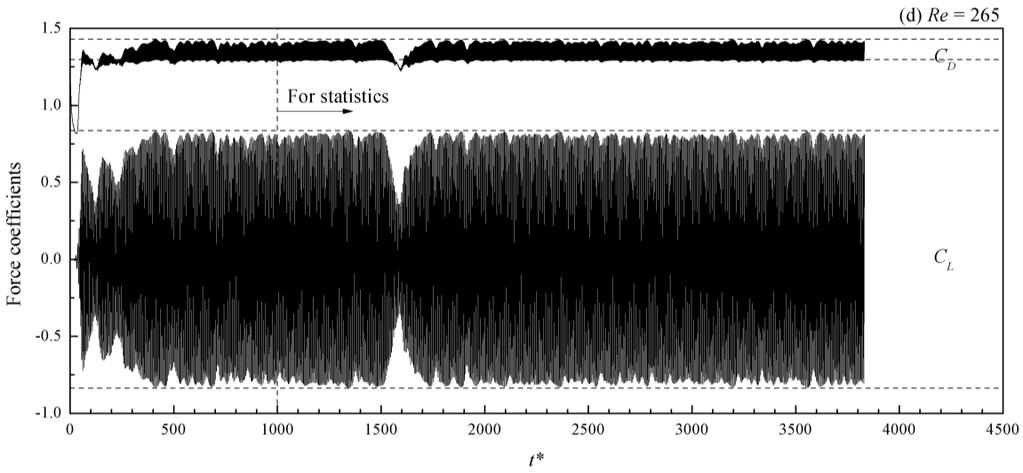
30 Dislocations No dislocation Starting point of a dislocation cycle Starting point of a non-dislocation cycle Re = 230 Re = 235 Re = 240 Re = 245 Re = 250 Re = 255 Re = 260 Re = t* Fig. 15. Time-histories of the occurrence of dislocations for the cases in the transition process from Mode A* to Mode B Time-histories of the force coefficients and vorticity Fig. 16 plots the time-histories of the drag and lift force coefficients for a few cases that contain Mode B. The horizontal dashed lines in each figure mark the fluctuation ranges of the corresponding 2D force coefficients. For the cases in the transition process from Mode A* to Mode B (Fig. 16(a c)), it is seen that the periods over which large amplitudes of C L take place match the non-dislocation periods shown in Fig. 15. The amplitudes of C D and C L observed during the non-dislocation periods are close to their 2D counterparts, indicating that the flow three-dimensionality is weak when dislocations do not occur. During the dislocation 30

31 periods, the C D values and the amplitudes of C L decrease, indicating that energy is transferred to the third direction. In particular, oblique vortex shedding occurs spontaneously along the entire span at t* = for the Re = 250 case (e.g. Fig. 17(a), in comparison with an example of parallel vortex shedding shown in Fig. 17(b)). Due to the remarkable phase differences along the span, the integrated lift coefficient is largely cancelled out, resulting in the smallest fluctuation amplitudes in the time-history (Fig. 16(b)). 31

32 32

33 Fig. 16. Time-histories of the drag and lift coefficients for some cases containing Mode B. (a) (b) Fig. 17. Iso-surfaces of ω x = ±0.5 at Re = 250: (a) oblique vortex shedding at t* = 33

34 3750, and (b) parallel vortex shedding at t* = Dark and light grey denote positive and negative values, respectively. The flow is from the left to the right past the cylinder on the left. The relationship between dislocation and the degree of flow three-dimensionality is further examined with both the largest ω x value in the domain and the streamwise enstrophy ε x integrated over the near-wake region of x/d = At Re = 240, for each of the three non-dislocation periods shown in Fig. 15, there is a sudden drop in the time-histories, as highlighted with a circle in the left column of Fig. 18. At Re = 260, each of the four dislocation periods corresponds to a rapid increase of ω x max and ε x, as circled in the middle column of Fig. 18. The non-dislocation and dislocation parts can be roughly divided by the horizontal line of ω x max = 4.5 as shown in Fig. 18(a). For the Re = 265 case, the entire time-histories beyond the only dislocation period of t* = are generally below the division line, as shown in the right column of Fig. 18. (a) 9 8 Re = 240 Re = 260 Re = x max (b) t* Re = t* t* Re = 260 Re = x t* t* t* 34

35 Fig. 18. Time-histories of (a) the largest ω x value in the domain, and (b) the streamwise enstrophy ε x integrated over the near-wake region of x/d = 0 10, for some cases in the transition process from Mode A* to Mode B. During the transition process from Mode A* to Mode B, the Mode B structure, which is largely observed in the non-dislocation segments with large-amplitude force coefficients, usually takes up part of the span and the streamwise vortices are quite ordered (e.g. Fig. 14(c,e)). At Re of 265 (beyond the only dislocation period) and 270, the large-amplitude force coefficients resemble the 2D results for the entire fully developed stage (Fig. 16(d,e)). The Mode B structure is also in an ordered pattern, and can normally occupy the majority of the span. Beyond Re = 270, Mode B becomes increasingly disordered with increase of Re. Correspondingly, the force coefficients deviate more and more from their 2D counterparts and become increasingly disordered (Fig. 16(f,g)). As Mode B becomes increasingly disordered beyond Re = 270, the largest ω x value and integrated ε x in the domain, which represent the degree of flow three-dimensionality, also increase with increase of Re (Fig. 19). Generally speaking, the streamwise vortices are found to be more disordered when ω x max > 5.5. It is seen from Fig. 19 that disordered Mode B can sometimes occur at Re = 280 (when ω x max > 5.5). Fig. 20 gives some examples of typical ordered and relatively disordered Mode B patterns at Re = 280. The corresponding ω x max values of the two time instants are pointed out in Fig. 19. For the ordered one shown in Fig. 20(a), the streamwise vortices are all parallel to each other in the streamwise direction and have similar spanwise wavelengths. In contrast, the disordered Mode B as shown in Fig. 20(b) contains slightly oblique streamwise vortices and their spanwise wavelengths are rather different. At Re = 300, disordered Mode B similar to the pattern shown in Fig. 20(b) occurs more frequently, whereas relatively ordered Mode B structures (e.g. Fig. 5) only occur occasionally. In this case, the majority part of the time-history of ω x max shown in Fig. 19(a) is above the horizontal line of ω x max =

36 (a) 8 7 Fig. 20(b) Re = 265 Re = 280 Re = x max Fig. 20(a) (b) t* Re = 265 Re = 280 Re = 300 x Fig. 20(b) Fig. 20(a) t* Fig. 19. Time-histories of (a) the largest ω x value in the domain, and (b) the streamwise enstrophy ε x integrated over the near-wake region of x/d = 0 10, for some cases beyond the transition process from Mode A* to Mode B. (a) (b) 36

37 Fig. 20. Iso-surfaces of ω x = ±0.5 at Re = 280: (a) ordered Mode B at t* = 1550, and (b) relatively disordered Mode B at t* = Dark and light grey denote positive and negative values, respectively. The location of the largest ω x value in the domain is denoted by a circle. The flow is from the left to the right past the cylinder on the left Critical condition at Re = Williamson (1996b) reported a critical condition at Re = 260 where maximum values of the base pressure coefficient and root-mean-square flow velocity were observed. The critical condition is confirmed in the present study at approximately Re = in terms of various quantities including flow velocity, vorticity, and hydrodynamic forces. Fig. 21(a) shows the variation of the time-averaged ω x max calculated from the time-histories (e.g. Fig. 18(a) and Fig. 19(a)) with Re. For Re 250, as mentioned previously, the relatively large ω x max values (i.e. strong flow three-dimensionality) are due to large-scale dislocations. A sharp drop of the ω x max is observed at Re = , in line with a sharp decrease of the probability of occurrence of dislocations as shown in Fig. 13. The averaged ω x max values obtained from a dislocation period and two non-dislocation periods (as shaded in Fig. 18) are further plotted in Fig. 21 to clarify the sharp drop. The non-dislocation periods that consist of either ordered Mode B or Mode A induce the lowest averaged ω x max values which are close to the one observed at Re = 270. In contrast, the averaged ω x max value observed during the dislocation period is much larger and is similar to the value observed in the dislocation period of Re = 240 (as indicated by the shaded rectangle in the left column of Fig. 18). However, because the probabilities of occurrence of dislocations for Re = 260 and Re = 240 have a drastic difference (21.2% and 88.0%, respectively), the overall averaged ω x max is very close to the dislocation value for Re = 240, but much closer to the non-dislocation values for Re = 260. At Re = 265, dislocations only have a very small probability of occurrence of 3.5% and thus only have a very small effect on the overall performance. Beyond Re = 270, there is no dislocation in the domain, 37

38 whereas the increasingly disordered Mode B becomes the reason why the averaged ω x max starts to grow again. Fig. 21(b,c) shows the variations of the time-averaged ε x and E z within x/d = 0 10 of the wake with Re. It is seen that all of the three quantities share similar trends in terms of predicting the three-dimensionality of the flow. (a) 7 6 Re = 240, t* = Re = 265, t* > 1800 Re = 260, t* = Entire range Re = 260, t* = Re = 260, t* = Time-averaged x max Re (b) Re = 240, t* = Re = 260, t* = Re = 260, t* = Re = 260, t* = Re = 265, t* > 1800 Entire range Time-averaged x Re 38

39 (c) Re = 240, t* = Re = 265, t* > 1800 Re = 260, t* = Entire range Re = 260, t* = Re = 260, t* = Time-averaged E z Re Fig. 21. Time-averaged quantities for the 3D cases: (a) the largest ω x value in the domain, (b) the integrated streamwise enstrophy within x/d = 0 10, and (c) the integrated spanwise kinetic energy within x/d = Fig. 22 shows the time-averaged drag coefficient and root-mean-square lift coefficient for a wide range of Re. The statistics is taken after the flow becomes fully developed. For the time-histories shown in Fig. 16, the statistics starts at t* = The results calculated from the second half of the sampling period are also plotted in Fig. 22 to demonstrate the sufficiency of the statistical data. At Re = 194, the deviations of the 3D C D and C L results from the 2D curves mark the onset of Mode A* instability. It is seen in Fig. 22 that the flow three-dimensionality becomes weakest at Re of 265 and 270, in line with the variation trends of the time-averaged ω x max, ε x, and E z (Fig. 21). The C D and C L values at Re = 260 can also be separated into the dislocation and non-dislocation parts (Fig. 22), in the same way as the separation of the time-averaged ω x max, ε x and E z values. 39