EECS490: Digital Image Processing. Lecture #23

Transcription

1 Lecture #23 Motion segmentation & motion tracking Boundary tracking Chain codes Minimum perimeter polygons Signatures

2 Motion Segmentation P k Accumulative Difference Image Positive ADI Negative ADI (ADI) for a moving rectangle. A k ( x, y)= A k 1( x, y)+ 1 if R( x, y) f( x, y, k) > T A k 1 ( x, y) otherwise The accumulator is incremented if the absolute difference between the reference frame and each successive frame is above a threshold. We can also have positive and negative accumulator images. ( x, y)= P x, y k 1( )+ 1 if R ( x, y ) f ( x, y,t k ) > T N k ( x, y)= N k 1( x, y )+ 1 if R ( x, y ) f x, y,t k P k 1 ( x, y) otherwise N k 1 ( x, y) otherwise ( ) < T

3 Image Segmentation How do you construct a static reference image if something is always is motion?

4 People Counter EECS490: Digital Image Processing

5 Boundary Tracking Assumptions: 1. The image is binary where 1=foreground and 0=background 2. The image is padded with a border of 0 s so an object cannot merge with the border. 3. There is only one object in this example. Moore Boundary Tracking Algorithm [1968]: 1. Start with the uppermost, leftmost foreground point b 0 in the image. Let c 0 be the west neighbor of b 0. Going clockwise from c 0 identify the first non-zero neighbor b 1 of b 0. Let c 1 be the background point immediately preceding b 1 in the sequence. 2. Let b=b 1 and c=c Let the 8-neighbors of b starting at c and proceeding clockwise be denoted as n 1, n 2,, n 8. Find the first n k which is foreground (i.e., a 1 ). 4. Let b=n k and c=n k Repeat steps 3 and 4 until b=b 0 and the next boundary point found is b 1. The sequence of b points found when the algorithm stops is the set of ordered boundary points.

6 Boundary Tracking The Moore boundary following algorithm repeats until b=b 0 and the next boundary point found is b 1. This prevents errors encountered in spurs. Simply finding b 0 again is not enough. For example, in this figure the algorithm would start at b 0, find b, and then come back to b 0 stopping prematurely with only b=b 0. However, the next boundary point found should be the circled point which is NOT b 1. Adding and the next boundary point found is b 1 will cause the algorithm to traverse the lower part of the object.

7 Chain Codes Examples of chain code direction numbers. A Freeman chain code represents a boundary as a connected sequence of straight line segments of specified direction and length.

8 Chain Codes Arbitrarily start chain code here 8-direction chain coded boundary Using original pixels usually results in a code which is too long and subject to noise Resample original image on a larger grid to reduce code size. 8-connected code:

9 Chain Codes 4-direction chain coded boundary Arbitrarily start chain code here 4-connected code: One practice is to rotate (pick start) to get smallest integer code. (START CODE HERE) Between end and start of boundary Chain codes can be normalized for rotation by using first differences. To compute the first difference go in counter-clockwise direction and find number of 90 rotations of direction. 1-> rotations ccw 0-> rotation ccw 1-> rotations ccw 0-> rotations ccw 3-> rotations ccw 3-> rotations ccw 2-> rotations ccw 2-> rotations ccw 4-connected difference code:

10 Noisy 570x570 image Chain Codes 9x9 averaging mask Otsu thresholded Single-point from Otsu thresholding (ignored) 8-directed chain code: Minimum magniture integer: First difference: Longest outer boundary Resampled on a 50x50 pixel grid Joining resampled pixels by straight lines

11 Minimum-Perimeter Polygon The goal is to represent the shape in a given boundary using the fewest possible number of sequences. Object boundary (binary image) Enclose boundary in a grid Allow boundary to shrink. The vertices of the polygon are all inner or outer corners of the grid.

12 Minimum-Perimeter Polygon convex convex The boundary cells from the previous slide enclose the circumscribed shape. Concave Concave mirror Traverse the 4-connected boundary of the circumscribed shape. Concave vertices on this boundary have mirrors on the outer boundary. The boundary is described by inner convex and outer concave vertices.

13 Minimum-Perimeter Polygon MPP Observations: 1. The MPP bounded by a simply connected cellular complex is not self-intersecting. 2. Every convex vertex of the MPP is a W vertex, but not every W vertex of a boundary is a vertex of the MPP. 3. Every mirrored concave vertex of the MPP is a B vertex, but not every B vertex of a boundary is a vertex of the MPP. 4. All B vertices are on or outside the MPP, and all W vertices are on or inside the MPP. 5. The uppermost, leftmost vertex in a sequence of vertices contained in a cellular complex is always a W vertex of the MPP. MPP convex Mirrored concave Cellular complex Not all vertices in the MPP become vertices of the MPP

14 Minimum-Perimeter Polygon Let a=(x 1,y 1 ), b=(x 2,y 2 ), and c=(x 3,y 3 ) A = x 1 y 1 1 x 2 y 2 1 x 3 y 3 1 sgn( a,b,c)= det( A)= > 0 if (a,b,c) is a counterclockwise sequence = 0 if (a,b,c) are collinear < 0 if (a,b,c) is a clockwise sequence

15 Minimum-Perimeter Polygon Definitions: Form a list whose rows are the coordinates of each vertex and whether that vertex is W or B. The concave verttices must be mirrored, the vertices must be in sequential order, and the first uppermost, leftmost vertex V O is a W vertex. There is a white crawler (W C ) and a black crawler (B C ). The Wc crawls along the convex W vertices, and the B C crawls along the mirrored concave B vertices.

16 Minimum-Perimeter Polygon MPP Algorithm: 1. Set W C =B C =V O 2. (a) V K is on the positive side of the line (V L,W C ) [sgn(v L,W C,V K )>0 (b) V K is on the negative side of the line (V L,W C ) or is collinear with it [sgn(v L,W C,V K ) 0; V K is on the positive side of the line (V L,B C ) or is collinear with it [sgn(v L,B C,V K ) 0 (c) V K is on the negative side of the line (V L,B C ) [sgn(v L,B C,V K )<0 If condition (a) holds the next MPP vertex is W C and V L =W C ; set W C =B C =V L and continue with the next vertex. If condition (b) holds V K becomes a candidate MPP vertex. Set W C =V K if V K is convex otherwise set B C =V K. Continue with next vertex. If condition (c) holds the next vertex is B C and V L =B C. Re-initialize the algorithm by setting W C =B C =V L and continue with the next vertex after V L. 3. Continue until the first vertex is reached again.

17 Minimum-Perimeter Polygon V 0 (1,4) W V 1 (2,3) B V 2 (3,3) W V 3 (3,2) B V 4 (4,1) W V 5 (7,1) W V 6 (8,2) B V 7 (9,2) B The fundamental concept is to move the crawlers along the perimeter, calculate the curvatures, and determine if the vertex is a vertex of the MPP. W C B C V L W C curvature B C curvature V 0 V 0 V 0 V 1 V 0 V 0 V 0 V L,W C,V 1 =0 V L,W B,V 1 =0 V 2 V 0 V 1 V 0 V L,W C,V 2 =0 V L,W B,V 2 >1 V 3 V 2 V 1 V 0 V L,W C,V 3 <0 V L,W B,V 3 =0 V 4 V 2 V 3 V 0 V L,W C,V 4 <0 V L,W B,V 4 =0 V 5 V 4 V 3 V 4 V L,W C,V 5 >0 V 5 V 4 V 4 V 4 V L,W C,V 5 =0 V L,W B,V 5 =0 V 6 V 5 V 4 V 4 V L,W C,V 6 >0 V 7 V 5 V 6 V 5 V L,W C,V 7 =0 V L,W B,V 7 =0

18 Minimum Perimeter Polygon 8-connected boundary MPP resampled 2x2, 206 vertices 566x566 binary image MPP resampled 3x3, 160 vertices MPP resampled 6x6, 92 vertices MPP resampled 4x4, 127 vertices MPP resampled 8x8, 66 vertices MPP resampled 16x16, 32 vertices MPP resampled 32x32, 13 vertices

19 Boundary Splitting Subdivide a segment successively until a specified criterion is satisfied 1. Identify the two most distant points joined by ab 2. Identify the most distant point up from ab 3. Identify the most distant point down from ab

20 Signatures A signature is a 1-D representation of a boundary Signatures can be made invariant to translation but may be sensitive to rotation and scale. These signatures are r- but there are others such as (tangent)-s. Methods of selecting starting point can make signature independent of rotation 1. Select point farthest from centroid 2. Select point farthest from centroid along eigenaxis 3. Use a chain code

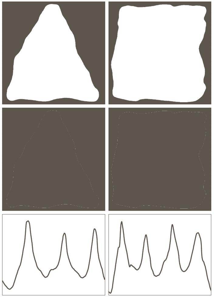
21 Signatures

22 Representation and Description The convex deficiency H-S The convex hull H The boundary of the object can be coded by the points where the boundary passes in and out of a convex deficiency

23 Median Axis Transformation Reduce the structure of a shape to a skeleton. However, as seen in our previous examples a morphological skeleton will not necessary be connected. Median Axis Transformation (MAT) of a region R with border B (guarantees connectivity of the skeleton) 1. For each point p in R find its closest* neighbor on B 2. If p has more than one closest * neighbor it belongs to the medial axis (skeleton) of B * Closest is defined using Euclidian distance

24 Thinning A suitable thinning algorithm is computationally MUCH faster that the MAT. Definitions A border point is any pixel with value 1 and at least one 8-connected neighbor with value 0. N(p 1 ) is the number of non-zero neighbors of p 1, i.e., N(p 1 )=p 2 +p 3 + +p 8 +p 9 T(p 1 ) is the number of 0->1 transitions in the ordered sequence p 1 p 2 p 3 p 9 p 2 p 1 is a boundary point N(p 1 ) = 4 T(p 1 ) = 3

25 Representation and Description Algorithm for thinning binary images Step 1. Mark for deletion any border point which has all of the following: (a) 2 N(p 1 ) 6 % don t delete if p 1 is an end point or inside region (b) T(p 1 )=1 % prevents breaking lines (c) p 2 p 4 p 6 =0 % (c) and (d) say that either p 2 AND p 8 are 0 (d) p 4 p 6 p 8 =0 % or p 4 or p 6 are 0, i.e., not part of the skeleton Step 2. Mark for deletion any border point which has all of the following: (a) 2 N(p 1 ) 6 % don t delete if p 1 is an end point or inside region (b) T(p 1 )=1 % prevents breaking lines (c) p 2 p 4 p 8 =0 % (c) and (d) say that either p 4 AND p 6 are 0 (d) p 4 p 6 p 8 =0 % or p 2 OR p 8 are 0, i.e., not part of the skeleton Iterate by applying Step 1 to all border points and deleting marked points. Then apply Step 2 to all remaining border points and delete marked points. Continue until no further points are deleted.

26 Representation and Description Double branch since wider than left side Skeletonized ( thinned ) image.

27 Representation and Description 4-direction chain code To compute the first difference go in counter-clockwise direction and find number of 90 rotations of direction. The shape number n is the smallest magnitude first difference chain code. n is even for closed boundaries

28 Representation and Description Definitions: Diameter = max[d(p i ),D(p j )] where p i and p j are points on the boundary. Major axis is the line segment of length equal to the diameter and connecting two points on the boundary. Minor axis is the line perpendicular to the major axis and of such length that a box passing through the outer four points of intersection of the boundary and the major/minor axes completely enclose the boundary This box enclosing the boundary is called the basic rectangle. Eccentricity is the ratio of major to minor axis.

29 Representation and Description 1. The major and minor axes 2. The basic rectangle 3. Use the rectangle with n=18 (given) which best approximates the shape of basic rectangle, i.e., 6x3= Resample boundary or use polygonal approximation 5. Computer chain code, its first difference, and the corresponding shape number.

30 Fourier Boundary Descriptors 1. Represent each point on a digital boundary as s k ( )= x k ( )+ jy x ( ) 2. Compute the DFT of the set of boundary points au ( )= 1 K K 1 s( k)e j 2 uk K,u = 0,1,2,...,K 1 k =0 3. The coefficients a(u) are the Fourier descriptors of the boundary K 1 s( k)= au ( )e + j 2 uk K u =0 Since K can be large we usually approximate the boundary by a smaller set of points, i.e., P, so that P 1 s( k) ŝ( k)= au ( )e + j 2 uk K u =0

31 Fourier Boundary Descriptors There are the same number of points in each reconstructed boundary but only the first P terms of the Fourier boundary descriptor were used to reconstruct the boundary. Basically, this is low-pass filtering of the shape.

32 Fourier Boundary Descriptors Fourier shape reconstruction using the first P=1434, 286, 144, 72, 36, 18 and 8 terms respectively.

33 Fourier Boundary Descriptors Shifts the DC (k=0) term Multiplies each term in a known way Rotation, scale, and translation of a boundary have simple effects on the Fourier description of that boundary.

34 Moments Connect start and stop points and compute perpendicular displacement from this line Can compute the mean displacement m and higher order moments n μ n m = K 1 r i i=0 ( ) gr i K 1 ( ) n ( r)= r i m i=0 gr ( i )

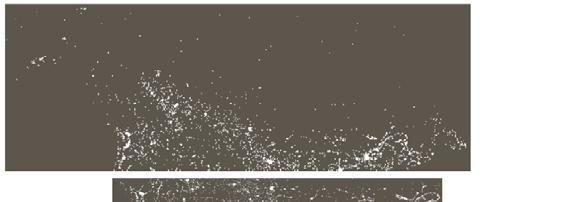
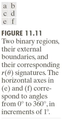
35 Other Representations Use ratio of white pixels to total area to estimate electrical energy consumption.

36 Topology Topology - properties that are unaffected by rubber sheet deformations The set of pixels that are connected to any pixel in S is called a connected component of S

37 Representation and Description E=C-H=1-1=0 E=C-H=1-2=-1 Euler number E=C-H C is the number of connected components; H is the number of holes

38 Representation and Description This polygonal network has: 7 vertices 11 edges 2 faces 3 holes 1 connected region Euler number E=V-Q+F V is the number of vertices Q is the number of edges F is the number of faces E=V-Q+F=7-11+2=-2

39 Representation and Description Single infrared image Result of thresholding (largest T before river becomes disconnected) gives 1591connected components Single component with largest number of pixels (8479) Computed skeleton of this component useful for computing length of river branches, etc.