Lecture 7 Measurement Using a Single Camera. Lin ZHANG, PhD School of Software Engineering Tongji University Fall 2016

Transcription

1 Lecture 7 Measurement Using a Single Camera Lin ZHANG, PhD School of Software Engineering Tongji University Fall 2016

2 If I have an image containing a coin, can you tell me the diameter of that coin?

3 Contents Foundations of Projective Geometry Matrix Differentiation Lagrange Multiplier Least squares for Linear Systems What is Camera Calibration Single Camera Calibration Bird s eye view Generation

4 Vector operations Vector representation a xi yjzk {, x y,} z Length (or norm) of a vector a x y z Normalized vector (unit vector) a { x, y, z } a a a a We say a 0, if and only if x 0, y 0, z 0

5 Vector operations a ( x, y, z ), b ( x2, y2, z2), ab ( x x, y y, z z ), if then b a ab a b cos x x y y z z Dot product (inner product) Laws of dot product: Theorem ab ba, a( b c)= ab+ ac ab 0 a b (why?)

6 Vector operations Cross product i j k ab x1 y1 z1 i j k x y z y z z x x y y z z x x y

7 Vector operations Cross product c a b is also a vector, whose direction is determined by the right hand law and c a, c b c a b sin c represents the oriented area of the parallelogram taking and a as two sides b (easy to prove) r r r r (why?) c b a

8 Vector operations Cross product Theorem Theorem ab,, same time, and ab ab0 (why?) they are not equal to zero at the (easy to understand) a b 0 Property r ( r r ) r r r r

9 Vector operations Mixed product (scalar triple product or box product) ( abc,, ) ( ab) c a a a b b Geometric Interpretation: it is the (signed) volume of the parallelepiped defined by the three vectors given b c c c

10 Vector operations Mixed product (scalar triple product or box product) ( abc,, ) ( ab) c a a a b b b c c c ( ab) c ab c cos absin ccos Base h c a

11 Vector operations Mixed product (scalar triple product or box product) ( abc,, ) ( ab) c Property: a a a b b b c c c ( abc,, ) ( bca,, ) ( cab,, ) ( abc,, ) ( bac,, ) ( acb,, ) why?

12 Vector operations Mixed product (scalar triple product or box product) Theorem abcare,, coplanar ( abc,, ) 0 why? abcare,, coplanar,, v, at the same time, and a bvc 0 they are not equal to zero

13 Foundations of Projective Geometry What is homogeneous coordinate? x, y, 0 T,,1, For a normal point on a plane kx y T Its homogenous coordinate is where k can be any non zero real number Homogenous coordinate for a point is not only one For a homogenous coordinate we usually rewrite it as x, y, z ' ' ' T ' ' ' ' x / z, y / z,1 T

14 Foundations of Projective Geometry What is homogeneous coordinate? For a normal point on a plane 0 Its homogenous coordinate is T k x, y,1, where k can be any non zero real number Converting from homogenous coordinate to inhomogeneous coordinate x ' T x, y, x z ' ' y ' ' y z ' z '

15 1 Foundations of Projective Geometry What is homogeneous coordinate? Geometric interpretation e 3 o 1 o e 2 M ( x, y ) e 1 e 2 e In plane, in the 2D frame, one point M :( x, y ) ( o : e, e ) Coordinate of any point on line OM in the frame ( o: e1, e2, e3) is the homogeneous coordinate of M These points can be represented as k x, y,1 T 0 0

16 1 Foundations of Projective Geometry What is homogeneous coordinate? Geometric interpretation e 3 o 1 o e 2 M ( x, y ) e 1 e 2 e In plane, in the 2D frame, one point M :( x, y ) ( o : e, e ) Coordinate of any point on line OM in the frame ( o: e1, e2, e3) is the homogeneous coordinate of M These points can be represented as k x, y,1 T 0 0 How about a line passing through O and parallel to 0?

17 Foundations of Projective Geometry What is homogeneous coordinate? Geometric interpretation e 3 How about a line passing through O and parallel to? 0 1 o 1 o e 2 e 1 e 2 M ( x, y ) Consider a line passing through O and M(x 0, y 0, 0) T We define: it meets 0 at an infinity e point, and also the homogeneous 1 coordinate of such a point can be represented as points on OM So, infinity point has the form (kx 0, ky 0, 0) T

18 Foundations of Projective Geometry What is homogeneous coordinate? Normal case: abnormal case: line k (x 0, y 0, 1) a normal point (x 0, y 0 ) on the plane 0 make an analogy line (kx 0, ky 0, 0) Define: it meets 0 at an infinity point The homogeneous coordinate of this normal point is k(x 0, y 0,1) The homogeneous coordinate of this infinity point is k(x 0, y 0,0)

19 Foundations of Projective Geometry What is homogeneous coordinate? Geometric interpretation e 3 How about a line passing through O and parallel to? 0 1 o 1 e 2 e 1 e 2 0 One infinity point determines an orientation We define: all infinity points on M ( x0, y0) o e comprise an infinity line 1 In fact, plane oee 1 2meets 0 at the infinity line Homogeneous equation of the infinity line is 0x + 0y + 1z = 0 0

20 Foundations of Projective Geometry 0 + infinity line = Projective plane Properties of a projective plane Two points determine a line; two lines determine a point (the second claim is not correct in the normal Euclidean plane) Two parallel lines intersect at an infinity point; that means one infinity point corresponds to a specific orientation Two parallel planes intersect at the infinity line

21 Foundations of Projective Geometry

22 Foundations of Projective Geometry JingHu High speed railway: rails will meet at the vanishing point

23 Foundations of Projective Geometry Lines in the homogeneous coordinate On a projective plane, please determine the line passing two ' points T T x ( x, y, z ), x ( x, y, z ) x M ' x 0 ox, o ' x determine two lines xx actually is the intersection between oxx and 0 1 e 2 o e 1

24 Foundations of Projective Geometry Lines in the homogeneous coordinate On a projective plane, please determine the line passing two ' points T T x ( x, y, z ), x ( x, y, z ) e 2 o x M e 1 ' x 0 Thus, M ( x, y, z) locates on xx om resides on the plane oxx ' ox, om, ox are coplanar x y z x y z x y z

25 Foundations of Projective Geometry Lines in the homogeneous coordinate On a projective plane, please determine the line passing two ' points T T x( x1, y1, z1), x ( x2, y2, z2) x y z y z z x x y x1 y1 z x 1 1 y 1 1 z y2 z2 z2 x2 x2 y2 x y z y z z x x y,, y z z x x y Homogeneous coordinate of the line Homogeneous coordinate of the infinity line is (0,0,1) T T 0

26 Foundations of Projective Geometry Lines in the homogeneous coordinate On a projective plane, please determine the line passing two ' points T T x( x1, y1, z1), x ( x2, y2, z2) x y z y z z x x y x1 y1 z x 1 1 y 1 1 z y2 z2 z2 x2 x2 y2 x y z Theorem xx, On the projective plane, the line passing two points is l x x ' y z z x x y,, y z z x x y T 0 '

27 Foundations of Projective Geometry Lines in the homogeneous coordinate x ( x, y, z ) T A point is on the line xl T (It is xl 0 ) l ( abc,, ) T

28 Foundations of Projective Geometry Lines in the homogeneous coordinate Theorem: On the projective plane, the intersection of two ' ' lines is the point ll, Proof: Two lines ax 1 by 1 cz 1 0, Inhomogeneous form, ax 1 by 1 c1 0 X ax 2 by 2 c2 0 x l l ax 2 by 2 cz 2 0 l T ' ( a1, b1, c1), l ( a2, b2, c2) x y X Y z z cb ac c b a c, Y ab ab a b a b T

29 x Foundations of Projective Geometry Lines in the homogeneous coordinate Theorem: On the projective plane, the intersection of two ' ' lines ll, is the point x l l Homogenous form of the cross point is cb 1 1 a1c1 cb 2 2 a2 c2 k,,1 ab 1 1 ab 1 1 ab 2 2 ab 2 2 x let bc 1 1 ca 1 1 ab 1 1,, b c c a a b k ab 1 1 a b 2 2 cb 1 1 a1c1 ab 1 1 x,, c2 b2 a2 c2 a2 b2 x ll '

30 Foundations of Projective Geometry Lines in the homogeneous coordinate Theorem: On the projective plane, the intersection of two ' ' lines is the point ll, x l l Example: find the cross point of the lines x1, y 1 y Homogeneous form y 1 1x1 0 x2 ( 1) x3 0 0x1 1 x2 ( 1) x3 0 o x x 1 T T lines are (1,0, 1),(0,1, 1) Homogeneous coordinates of the two Cross point is (1, 0, 1) T T (0,1, 1) 1,1,1 x x x x, y x

31 Foundations of Projective Geometry Lines in the homogeneous coordinate Theorem: On the projective plane, the intersection of two ' ' lines is the point ll, x l l Example: find the cross point of the lines x1, x 2 y Homogeneous form x 2 1x1 0 x2 ( 1) x3 0 1x1 0 x2 ( 2) x3 0 o x T T lines are (1,0, 1),(1,0, 2) x 1 Cross point is i j k Homogeneous coordinates of the two T T (1,0, 1) (1,0, 2) ,1,0 102 x x x x, y x

32 Foundations of Projective Geometry Duality In projective geometry, lines and points can swap their positions T xl 0 How to interpret? If x is a variable, it represents the points lying on the line l; If l is a variable, it represents the lines passing a fixed point x xx, ll, The line passing two points is ' The cross point of two lines is ' l xx ' x ll Duality Principle: To any theorem of projective geometry, there corresponds a dual theorem, which may be derived by interchanging the roles of points and lines in the original theorem '

33 Contents Foundations of Projective Geometry Matrix Differentiation Lagrange Multiplier Least squares for Linear Systems What is Camera Calibration Single Camera Calibration Bird s eye view Generation

34 Matrix differentiation Function is a vector and the variable is a scalar f( t) f1( t), f2( t),..., f ( ) T n t Definition df df () t df () t dfn t,,..., dt dt dt dt 1 2 () T

35 Matrix differentiation Function is a matrix and the variable is a scalar Definition f11( t) f12( t),..., f1 m( t) f21( t) f22( t),..., f2m( t) f() t fij () t fn1() t fn2(),..., t fnm() t df dt nm df11() t df12() t df1 (),..., m t dt dt dt df21() t df22() t df2m() t,..., dfij () t dt dt dt dt dfn 1() t dfn2() t dfnm() t,..., dt dt dt nm

36 Matrix differentiation Function is a scalar and the variable is a vector Definition In a similar way, f x x x1 x2 x n ( ), (,,..., ) T df f f f,,..., dx x1 x2 x f x x x1 x2 x n ( ), (,,..., ) df f f f,,..., dx x1 x2 x n n T

37 Matrix differentiation Function is a vector and the variable is a vector T x x, x,..., x, y y ( x), y ( x),..., y ( x) Definition dy dx 1 2 n 1 2 T y1( x) y1( x) y1( x),,..., x1 x2 x n y2( x) y2( x) y2( x),,..., x1 x2 x n y ( x) y ( x) y ( x),,..., m m m x1 x2 xn mn m T

38 Matrix differentiation Function is a vector and the variable is a vector T x x, x,..., x, y y ( x), y ( x),..., y ( x) 1 2 n 1 2 In a similar way, dy dx T y1( x) y2( x) ym( x),,..., x1 x1 x 1 y1( x) y2( x) ym( x),,..., x2 x2 x 2 y1( x) y2( x) ym( x),,..., x x x n n n n m m T

39 Matrix differentiation Function is a vector and the variable is a vector Example: x y y y x x x 1 1( x) 2 2, x2, y1( ) x1 x2, y2( ) x3 3x2 2( x) x 3 y1( x) y2( x) x x 1 1 2x1 0 T dy y1( x) y2( x) 1 3 dx x x x3 y1( x) y2( x) x x 3 3

40 Matrix differentiation Function is a scalar and the variable is a matrix Definition df ( X) dx f ( X), X mn f f f x11 x12 x1 n f f f x x x m1 m2 mn

41 Matrix differentiation Useful results (1) Then, d dx T ax xa, n1 d a, dx T xa a How to prove?

42 Matrix differentiation Useful results mn n1 dax (2) A, x Then, A T dx (3) mn n1 A, x Then, T T dx A T A dx (4) T nn n1 dx Ax T A, x Then, ( A A ) x dx (5) T mn m1 n1 daxb X, a, b Then, ab dx T T nm m1 n1 daxb (6) X, a, b Then, ba dx T dxx n1 (7) x Then, 2x dx T T

43 Contents Foundations of Projective Geometry Matrix Differentiation Lagrange Multiplier Least squares for Linear Systems What is Camera Calibration Single Camera Calibration Bird view Generation

44 Lagrange multiplier Single variable function x0 ( ab, ) f ( x) is differentiable in (a, b). At, f(x) achieves an extremum df dx Two variables function 0 x 0 ( x, y ) f ( x, y) is differentiable in its domain. At 0 0, f(x, y) achieves an extremum f x f ( x0, y0) 0, ( x0, y0) 0 y

45 Lagrange multiplier In general case If x 0 is a stationary point of f ( x), x n1 f f f 0, 0,..., x x x x x x 1 2 n

46 Lagrange multiplier Lagrange multiplier is a strategy for finding the local extremum of a function subject to equality constraints Problem: find stationary points for y f( x), x under m constraints g ( x) 0, k 1, 2,..., m Solution: 1 k F( x;,..., ) f( x) g ( x) ( x,,..., m ) m k k k 1 is a stationary point of with constraints m If is a stationary point of F, then, x f ( x) 0 n1 Joseph Louis Lagrange Jan. 25, 1736~Apr.10, 1813

47 Lagrange multiplier Lagrange multiplier is a strategy for finding the local extremum of a function subject to equality constraints Problem: find stationary points for y f( x), x under m constraints g ( x) 0, k 1, 2,..., m Solution: F( x;,..., ) f( x) g ( x) 1 m m k k k 1 ( x0, 10,..., m 0) is a stationary point of F F F F F F F 0, 0,..., 0, 0, 0,..., 0 x x x 1 2 n 1 2 at that point k n + m equations! n1 m

48 Lagrange multiplier Example Problem: for a given point p 0 = (1, 0), among all the points lying on the line y=x, identify the one having the least distance to p 0. The distance is 2 2 f( x, y) ( x1) ( y0) y=x? Now we want to find the stationary point of f(x, y) under the constraint gxy (, ) yx0 According to Lagrange multiplier method, construct another function p 0 (,, ) ( ) ( ) ( 2 1) 2 ( ) F x y f x g x x y y x Find the stationary point for F( xy,, )

49 Lagrange multiplier Example Problem: for a given point p 0 = (1, 0), among all the points lying on the line y=x, identify the one having the least distance to p 0. F 0 x 2( x 1) 0 x 0.5 F 0? 2y 0 y y 0.5 x y 0 F 1 p 0 0 y=x (0.5,0.5,1) is a stationary point of (,, ) F xy (0.5,0.5)is a stationary point of f(x,y) under constraints

50 Contents Foundations of Projective Geometry Matrix Differentiation Lagrange Multiplier Least squares for Linear Systems Homograpy Estimation What is Camera Calibration Single Camera Calibration Bird view Generation

51 LS for Inhomogeneous Linear System Consider the following linear equations system x1x x1 3 2x1x x 2 4 A x b Matrix form: Ax b It can be easily solved x x

52 LS for Inhomogeneous Linear System How about the following one? x1x x1 2x1 x x 2 x1 2x It does not have a solution! What is the condition for a linear equation system can be solved? Ax b Can we solve it in an approximate way? A: we can use least squares technique! Carl Friedrich Gauss

53 LS for Inhomogeneous Linear System Let s consider a system of p linear equations with q unknowns a11x1 a12x2... a1 qxq b1 a x a x... a x b... a x a x... a x b q q 2 p1 1 p2 2 pq q p We consider the case: p>q, and rank(a)=q In general case, there is no solution! Ax Instead, we want to find a vector x that minimizes the error: p 2 E( ) ( ai 1x1... aiqxq i) A i1 x b xb 2 b unknowns

54 LS for Inhomogeneous Linear System * x arg min E( x) arg min Axb x x 2 2 x AA 1 A * T T b Pseudoinverse of A How about the pseudoinverse of A when A is square and non-singular?

55 LS for Homogeneous Linear System Let s consider a system of p linear equations with q unknowns a11x1 a12x2... a1 qxq 0 a21x1 a22x2... a2qxq 0... ap1x 1 ap2x 2... apqx q 0 We consider the case: p>q, and rank(a)=q Theoretically, there is only a trivial solution: x = 0 x 1 2 Ax 0 unknowns So, we add a constraint to avoid the trivial solution

56 LS for Homogeneous Linear System E( x) Ax We want to minimize, subject to 2 * x E x st x x arg min ( ),.., 1 Use the Lagrange multiplier to solve it, * 2 2 x arg min Ax 1 x 2 2 x 2 2 (1) x 1 2 Solving the stationary point of the Lagrange function, 2 2 Ax 1 x 2 2 x 2 2 Ax 1 x (3) (2)

57 LS for Homogeneous Linear System Then, we have Ax 1 x 2 2 x 2 2 T AAxx x is the eigen vector of A T A associated with the eigenvalue (3) T T T E x Ax x A Axx x The unit vector x is the eigenvector associated with the minimum T eigenvalue of A A

58 Contents Foundations of Projective Geometry Matrix Differentiation Lagrange Multiplier Least squares for Linear Systems Homograpy Estimation What is Camera Calibration Single Camera Calibration Bird s eye view Generation

59 Homography Estimation Problem definition: x x ' i Given a set of points i and a corresponding set of points in a projective plane, compute the projective transformation ' that takes to x i x i ' We know there existing an H satisfying xi Hxi, i 1,2,..., n Coordinates of and x are known, we need to find H x ' i i where H is a homography matrix a a a H a a a a a a It has 8 degrees of freedom

60 Homography Estimation 4 point correspondence pairs can uniquely determine a homography matrix since each correspondence pair solves two degrees of freedom cu a11 a12 a13 x cv a a a y c a31 a32 a 33 1 a xa ya a xa ya a xa ya a xa ya u v a11xa12 ya13 cu a21x a22 ya23 cv a31x a32 ya33 c

61 Homography Estimation 4 point correspondence pairs can uniquely determine a homography matrix since each correspondence pair solves two degrees of freedom a11 a12 a 13 a21 x y ux uy u a x y 1 vx vy v a23 Thus, four correspondence pairs a31 generate 8 equations a 32 a 33

62 Homography Estimation 4 point correspondence pairs can uniquely determine a homography matrix since each correspondence pair solves two degrees of freedom Ax (1) Normally, Rank( A) 8; thus (1) has 1 (9 8) solution vector in its solution space

63 Homography Estimation How about the case when there are more than 4 correspondence pairs? Use the LS method (for homogeneous case) to solve the model

64 Contents Foundations of Projective Geometry Matrix Differentiation Lagrange Multiplier Least squares for Linear Systems Homograpy Estimation What is Camera Calibration Single Camera Calibration Bird s eye view Generation

65 What is camera calibration? Camera calibration is a necessary step in 3D computer vision in order to extract metric information from 2D images It estimates the parameters of a lens and image sensor of the camera; you can use these parameters to correct for lens distortion, measure the size of an object in world units, or determine the location of the camera in the scene These tasks are used in applications such as machine vision to detect and measure objects. They are also used in robotics, for navigation systems, and 3 D scene reconstruction

66 What is camera calibration?

67 What is camera calibration? Camera parameters include Intrinsics Extrinsics Distortion coefficients

68 Contents Foundations of Projective Geometry Matrix Differentiation Lagrange Multiplier Least squares for Linear Systems Homograpy Estimation What is Camera Calibration Single Camera Calibration Bird s eye view Generation

69 Single Camera Calibration For simplicity, usually we use a pinhole camera model

70 Single Camera Calibration To model the image formation process, 4 coordinate systems are required World coordinate system (3D space) Camera coordinate system (3D space) Retinal coordinate system (2D space) Pixel coordinate system (2D space)

71 Single Camera Calibration To model the image formation process, 4 coordinate systems are required

72 Single Camera Calibration From the world CS to the camera CS T X, Y, Z is a 3D point represented in the WCS w w w In the camera CS, it is represented as, Xc Xw Yc R Yw Z c Z w 33 a rotation matrix (orthogonal) t a 31translation vector

73 Single Camera Calibration From the world CS to the camera CS T X, Y, Z is a 3D point represented in the WCS w w w In the camera CS, it is represented as, Xc Xw Yc R Yw Z c Z w t Homogeneous form X c X w R t Yc Yw T Z c 0 1 Z w 1 1 (1)

74 Single Camera Calibration From the camera CS to the retinal CS We can use a pin hole model to represent the mapping from the camera CS to the retinal CS

75 Single Camera Calibration From the camera CS to the retinal CS We can use a pin hole model to represent the mapping from the camera CS to the retinal CS f y z x O is the optical center, f is the focal length, P = [X c, Y c, Z c ] T is a scene point while P =(x, y) is its image on the retinal plane

76 Single Camera Calibration From the camera CS to the retinal CS X We can use a pin hole model to represent the mapping from the camera CS to the retinal CS X c c x Z c Y c y Y c Z f c Zc f Homogeneous form X c x f 000 Yc Z c y 0 f 00 Z c (2)

77 Single Camera Calibration From the retinal CS to the pixel CS The unit for retinal CS (x-y) is physical unit (e.g., mm, cm) while the unit for pixel CS (u-v) is pixel One pixel represents dx physical units along the x axis and represents dy physical units along the y axis; the image of the optical center is (u 0, v 0 ) 1 0 u0 dx u x 1 v 0 v 0 y dy

78 Single Camera Calibration From the retinal CS to the pixel CS If the two axis of the pixel plane are not perpendicular to each other, another parameter s is introduced to represent the skewness of the two axis 1 0 u0 dx u x 1 v 0 v 0 y dy s u0 dx u x 1 v 0 v 0 y dy (3)

79 Single Camera Calibration From Eqs.1~3, we can have 1 f s u0 sf u0 0 dx Xc 000 dx Xc u f 1 Yc f Yc Z c v 0 v 0. 0 f 00 0 v0 0. dy Z c dy Z c X c Xw Xw u0 0 u0 0 0 Yc 0 v0 0. R t u Yw Yw 0 v v0. R t Z T c 0 1 Z w Z w Intrinsic Extrinsic

80 u Single Camera Calibration X X u w w u 0 Yw Yw K [ R t] 0 0 [ R t] Z w Z w Zc v v , v Intrinsic Extrinsic 0 0, the coordinates of the principal point in the image plane and, the scale factors in image u and v axes, describing the skewness of the two image axes R and t determines the rigid transformation from the world coordinate system to the camera coordinate system Altogether, there are 11 parameters to be determined

81 Single Camera Calibration To accurately represent an ideal camera, the camera model can include the radial and tangential lens distortion Radial distortion occurs when light rays bend more near the edges of a lens than they do at its optical center; the smaller the lens, the greater the distortion

82 Single Camera Calibration To accurately represent an ideal camera, the camera model can include the radial and tangential lens distortion Radial distortion occurs when light rays bend more near the edges of a lens than they do at its optical center; the smaller the lens, the greater the distortion u u 1k r k r k r distorted v v 1k r k r k r distorted where r u v k, k, k are the radial distortion coefficients of the lens

83 Single Camera Calibration To accurately represent an ideal camera, the camera model can include the radial and tangential lens distortion Tangential distortion occurs when the lens and the image plane are not parallel

84 Single Camera Calibration To accurately represent an ideal camera, the camera model can include the radial and tangential lens distortion Tangential distortion occurs when the lens and the image plane are not parallel 2 2 u distorted u+ 21uv2 r 2u v v 2 uv r 2v distorted , 2 are the tangential distortion coefficients of the lens

85 Single Camera Calibration The purpose of the camera calibration is to determine the values for the extrinsics, intrinsics, and distortion coefficients How to do? Zhengyou Zhang s method [1] is a commonly used modern approach A calibration board is needed; several images of the board need to be captured; based on the correspondence pairs (pixel coordinate and world coordinate of a feature point), equation systems can be obtained; by solving the equation systems, parameters can be determined [1] Z. Zhang, A flexible new technique for camera calibration, IEEE Trans. Pattern Analysis and Machine Intelligence, 2000

86 Single Camera Calibration Calibration board

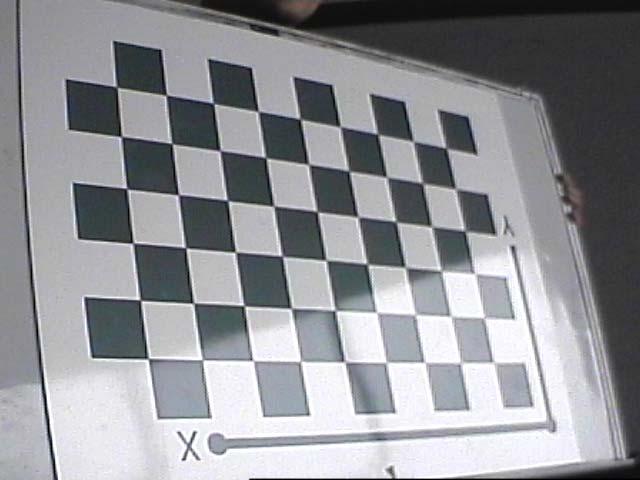
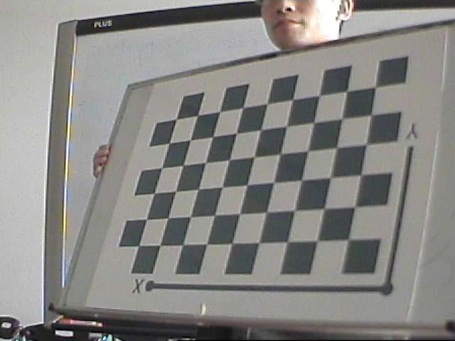
87 Single Camera Calibration A set of Calibration board images (50~60)

88 Single Camera Calibration Matlab provides a Camera Calibrator Straightforward to use However, based on my experience, it is not as accurate as the routine provided in opencv3.0, especially for large FOV cameras (such as fisheye camera); thus, for some accuracy critical applications, I recommend to use the opencv function, though a little more complicated It exports cameraparams as the calibration result

89 Single Camera Calibration

90 Single Camera Calibration For our purpose (measuring geometric metrics of a planar object), we use the camera parameters to undistort the image The essence of this step is to make sure the transformation from a physical plane to the image plane can be represented by a linear projective matrix; or in other words, a straight line should be mapped to a straight line

91 Single Camera Calibration Original image Undistorted image

92 Contents Foundations of Projective Geometry Matrix Differentiation Lagrange Multiplier Least squares for Linear Systems Homograpy Estimation What is Camera Calibration Single Camera Calibration Bird s eye view Generation

93 Bird s eye view Generation Our task is to measure the geometric properties of objects on a plane (e.g., conveyor belt) Such a problem can be solved if we have its bird view image; bird s eye view is easy for object detection and measurement

94 Bird s eye view Generation Three coordinate systems are required Bird s eye view image coordinate system World coordinate system Undistorted image coordinate system Y X X X Similarity Projective Y Y Bird s eye view image WCS Undistorted image

95 Bird s eye view Generation Basic idea for bird s eye view generation Suppose that the transformation matrix from bird s eye view to WCS is PB W and the transformation matrix from WCS to the undistorted image is PW I Then, given a position x,,1 T B yb on bird s eye view, we can get its corresponding position in the undistorted image as xb xi PWIPB W yb 1 Then, the intensity of the pixel x,,1 T B yb can be determined using some interpolation technique based on the neighborhood around on the undistorted image x I

96 Bird s eye view Generation Basic idea for bird s eye view generation Suppose that the transformation matrix from bird s eye view to WCS is PB W and the transformation matrix from WCS to the undistorted image is PW I P PW I The key problem is how to obtain B W and?

97 Bird s eye view Generation Determine P BW N (pixels) Y X H (mm) X M (pixels) Y

98 Bird s eye view Generation Determine P BW For a point xb yb on bird s eye view, the corresponding point on the world coordinate system is,,,1 T H HN 0 M 2M xw xb xb H H y W 0 yb PB W yb M Please verify!!

99 Bird s eye view Generation Determine W P I The physical plane (in WCS) and the undistorted image plane can be linked via a homography matrix P WI x x I PW I W N Ii Wii 1 If we know a set of correspondence pairs x, x, PW I can be estimated using the least square method

100 Bird s eye view Generation Determine W P I A set of point correspondence pairs; for each pair, we know its coordinate on the undistorted image plane and its coordinate in the WCS

101 Bird s eye view Generation When P BW and PW I are known, the bird s eye view can be generated via, x xb xb P P y P y 1 1 I W I B W B B I B

102 Bird s eye view Generation Original image Bird s eye view

103 Bird view Generation Another example Original fish eye image Undistorted image

104 Bird view Generation Another example Original fish eye image Bird s eye view

105 Thanks for your attention