UNIT 2. Translation/ Scaling/ Rotation. Unit-02/Lecture-01

Transcription

1 UNIT 2 Translation/ Scaling/ Rotation Unit-02/Lecture-01 Translation- (RGPV-2009,10,11,13,14) Translation is to move, or parallel shift, a figure. We use a simple point as a starting point. This is a simple operation that is easy to formulate mathematically. We want to move the point P1 to a new position P2. P 1 =(x 1,y 1 )=(3,3) P 2 =(x 2,y 2 )=(8,5) We see that x 2 =x 1 +5 y 2 =y 1 +2 This means that translation is defined by adding an offset in the x and y direction: tx and ty: x 2 =x 1 +tx y 2 =y 1 +ty We assume that we can move whole figures by moving all the single points. For a many-sided figure, a polygon, this means moving all the corners.

2 Scaling- Again we will use a single point as a starting point: P1. P 1 =(x 1,y 1 )=(3,3) We "scale" the point by multiplying it with a scaling factor in the x-direction, sx=2, and one in the y-direction, sy=3, and get P 2 =(x 2,y 2 )=(6,9) The relation is: x 2 =x 1 sx y 2 =y 1 sy It may seem a bit strange to say that we scale a point, since a point in a geometric sense doesn't have any area. It is better to say that we are scaling a vector. If we consider the operation on a polygon, we see that the effect becomes a little more complicated than with translation. In addition to moving the single points, the polygon's angles and area is also changed. Note: Scaling is expressed in relation to origin

3 Rotation- Rotation is more complicated to express and we have to use trigonometry to formulate it. P 1 =(x 1,y 1 )=(r cos(v 1 ),r sin(v 1 )) P 2 =(x 2,y 2 )=(r cos(v 1 +v 2 ),r sin(v 1 +v 2 )) We'll introduce the trigonometric formulas for the sum of two angles: sin (a+b) = cos(a) sin(b)+sin(a) cos(b) cos (a+b) = cos(a) cos(b)-sin(a) sin(b) and get: P 1 =((r cos(v 1 ), r sin(v 1 ) ) P 2 =(r cos(v 1 ) cos(v 2 )-r sin(v 1 ) sin(v 2 ), r cos(v 1 ) sin(v 2 )+r sin(v 1 ) cos(v 2 )) We insert: x 1 =r cos(v 1 ) y 1 =r sin(v 1 ) in P2's coordinates: P 2 =(x 2,y 2 )=(x1 cos(v 2 )-y1 sin(v 2 ), x1 sin(v 2 )+y1 cos(v 2 )) and we have expressed P2's coordinates with P1's coordinates and the rotation angle v. x 2 = x 1 cos(v)-y 1 sin(v) y 2 = x 1 sin(v)+y 1 cos(v) Notie: Rotation is expressed relative to origin. This also means that the sides in figures that are rotated create new angles with the axes after a rotation. We assume that the positive rotation angle is counterclockwise.

4 Matrices We now have the following set of equations that describes the three basic operations: Translation defined by tx and ty x 2 =x 1 +tx y 2 =y 1 +ty Scaling defined by sx and sy x 2 =sx x 1 y 2 =sy y 1 Rotation defined by v x 2 = x 1 cos(v)-y 1 sin(v) y 2 = x 1 sin(v)+y 1 cos(v) We want to find a common way to represent the operations. We know from linear algebra that we can represent linear dependencies like these with matrices. If we take the equation sets directly we get: Translation decided by tx and ty Scaling decided by sx and sy Rotation decided by v x2 x1 tx = + y2 y1 tx x2 sx 0 x1 = * y2 0 sy y1 x2 cos(v) -sin(v) x1 = * y2 sin(v) cos(v) y1 The matrix operations multiplication and addition are described in the module: Algebra. S.NO RGPV QUESTIONS Year Marks Q.1 Derive a general 2D-Transformation matrix for rotation about the origin. perform a 45 0 rotation of a square having vertices- A(0,0),B(0,2),C(2,2),D(2,0) about the origin. RGPV Q.2 RGPV Q.3 Find the new coordinates of the triangle A(0,0),B(1,1) and C(5,2) after it has been RGPV i)magnified to twice its size ii)reduced to half its size.

5 UNIT 2 Homogeneous coordinates /Shearing Unit-02/Lecture-02 Homogeneous coordinates- (RGPV-2003, 04, 06, 09, 11) The three basic operations have a little different form. We want the same form and introduce homogeneous coordinates. This means that we write a position vector like this: x y 1 Then we can write all basic operations as multiplication between a 3 x 3 matrix and a 1 x 3 vector. Translation Scaling Rotation x2 1 0 tx x1 y2 = 0 1 ty * y x2 sx 0 0 x1 y2 = 0 sy 0 * y x2 cos(v) -sin(v) 0 x1 y2 = sin(v) cos(v) 0 * y We have a general form P2=M P1 Where P1 and P2 are expressed in homogeneous coordinates. We will not worry about the third coordinate, the number 1. We'll not try to give a geometric explanation of this. The whole point is to standardize the mathematics in the transformations. The third coordinate stays the same in the basic transformations and, as we will se later, in combinations of them. The module Homogenizing discusses this subject a bit further. Geometry- We'll use this common form of expression for many things. But first, lets look at some simple relations between matrices and geometry. The identity matrix An important matrix is the identity matrix: I=

6 It transforms a point to itself: P1=P2=I P1 This can be interpreted as - translation with (0,0) - rotation with 0 degrees, since cos (0)=1 and sin (0) =0 - scaling with (1,1) We will need the identity matrix in many situations. In OpenGL there is a function to specify this as the current transformation matrix. glloadidentity () Later we will learn why this function is important. Mirroring We can mirror a point around the coordinate axes with matrices. Around the y-axis, a scaling with (-1,0): SY= Around the x-axis, a scaling with (0,-1): SX= Shearing A special operation called shearing is a scaling along one of the axes that depends on the coordinate on the other axis, for example the x-axis depends on y:

7 1 s 0 S= This is a representation of x2=x1+s y and y2=y1. The figure shows shearing used on a rectangle and with s=1. We notice that this is the effect we find in italic fonts. Projection We can project a point, for example onto the x-axis with the matrix I= In the plane we see that the only effect from this parallel projection is that it removes the y-coordinate. The consequence of this will always be a line along the x-axis. In space projections are more interesting. Compound operations- It is nice to have a common form for the basic transformations. We get the profit when we see how we can combine geometric operations by combining matrices. We can combine several geometric operations by multiplying the respective matrices. Before we do this, we can have a look at the advantages. They are essentially three: 1. Rendering speed. Typically we will be in a situation where we have to calculate coordinates for a large number of points, maybe thousands, when we represent our drawing on the screen. The coordinates for these points are changed by various reasons, and their position could be the result of a large number of geometric transformations. We want to decrease the number of calculations for every point. Instead of multiplying every vector (point) with all of the matrices that are involved in turn, we want to multiply it with only one matrix. It works like this in OpenGL: There is always a current model matrix that all of the points are multiplied with. 2. Modeling. We will return to this later. But let us indicate the problem for now by saying that we often have figures put together by different components. The different components are combined in a way that makes their position dependant of other parts of the figure. For example are the fingers on a robot dependant of the position of the arm they are attached to. Then it could be clever to reuse the transformations matrices several times. A practical way to do this is to have a stack of transformation matrices. This is the way it is done in OpenGL. 3. We can integrate the viewing transformation with the model transformation. Let s study some simple examples that illustrate the principle. Two translations We'll start with a simple example. Let us assume that we are doing two translations on a point. Let us assume that the first translation is (2,3) and that the second is (4,6). We can of course easily from geometrical

8 considerations establish that the result should be a translation (6,9). If not, something has to be wrong with our reasoning. The two matrices are: T1= and T2= and the product: T1*T2= We see that the result is as desired. We achieve a matrix that realizes the compound operations by multiplying the two single matrices. We also see that in this special case we could have gotten the matrix by adding the matrices as well, but this is a special case for two translations. We also see that in this case T1 T2=T2 T1. This is not surprising. It doesn't matter in what order the operations are done. However in general the matrix multiplication is not independent of the factor's order. This is a special case. We want to examine the relation between order and matrix multiplication closer in the next example. Rotation around another point than origin We consider a triangle with the corners a (1, 1), b (2,-1) and c (4, 2). We want to rotate this triangle 90 degrees around one of its corners, a. We know that rotation, as we described it above, always is performed around origin. We have to make a strategy that combines several transformations. We try two strategies and then try to draw some conclusions. A strategy could be: 1. Move origin to rotation corner 2. Rotate 90 degrees 3. Move origin back 4. It is easy to put up the three matrices that realize the three operations.

9 Move origin to the corner, a: Rotate 90 degrees: Move origin back: T1= R = T2= If we follow our reasoning we will get a matrix M=T1 R T2, and we should get the desired effect by multiplying all the points in the triangle with this matrix, P2=M P M = * * = * = We use M on the three points in the triangle and get: a' = M*a * 1 = b' = M*b * -1 = c' = M*c * 2 = and we can draw the result: Which is what we wanted. Our strategy was successful. An alternative strategy could be as follows:

10 1. Move the triangle so that a ends up in origin 2. Rotate 90 degrees 3. Move the triangle back, so that a ends up in its original place Since moving the point a to the origin is the opposite of moving the origin to a, the first operation is the same as what we called T2 above. In the same way step 3, moving the triangle back, is the same as what we called T1 above. The alternative strategy becomes: M=T2 R T1. If we calculate this we get: M = If we use this matrix on the triangle's three points we get a solution like this: which is not what we wanted. Above we found that moving the point to origin and moving origin to the point are opposite transformations. The same transformation matrices are a part of both strategies, but the order they are used in is different. We also saw that the first strategy with moving the origin was successful. This leads to the following formulation of a strategy to couple matrices to geometric reasoning. We can do either: 1. We can go through with the reasoning on the origin, and set up the matrices in the same order as we reason. 2. We can go through with the reasoning on the figure, and set up the matrices in the opposite order of the geometric reasoning. Normally we will use strategy 1, but some times it can be easier to reason with strategy 2. S.NO RGPV QUESTIONS Year Marks Q.1 Why are homogenous coordinate system used for transformation computation in computer graphics? Rgpv- 2005,09,11 Q.2 Explain shearing and reflection with example. Rgpv

11 UNIT 2 Transformations as matrices/ Composite Transformations Unit-02/Lecture-03 Transformations as matrices (rgpv-2007,09) Scale: xnew = sxxold ynew = syyold Rotation: x2 = x1cosθ - y1sin θ y2 = x1sin θ + y1cos θ Translation: xnew = xold + tx ynew = yold + ty Homogeneous Coordinates In order to represent a translation as a matrix multiplication operation we use 3 x 3 matrices and pad our points to become 3x 1 matrices. This coordinate system (using three values to represent a 2D point) is called homogeneous coordinates.

12 Composite Transformations: Suppose we wished to perform multiple transformations on a point: Remember: Matrix multiplication is associative, not commutative! Transform matrices must be pre-multiplied The first transformation you want to perform will be at the far right, just before the point. Composite Transformations -Scaling Given our three basic transformations we can create other transformations. A problem with the scale transformation is that it also moves the object being scaled. Scale a line between (2, 1) (4,1) to twice its length.

13 Fixed Point Scaling Scale by 2 with fixed point = (2,1) Translate the point (2,1) to the origin Scale by 2 Translate origin to point (2,1) S.N O RGPV QUESTIONS Year Marks Q.1 Give the transformation matrix for 2D rotation about any arbitrary point(r x, R y ). Rgpv Q.2 Magnify the triangle with vertices A(0,0),B(1,1) and C(5,2) to twice its size while keeping C(5,2) fixed. Rgpv 2014,2007,2008 7,10

14 UNIT 2 2D transformation Unit-02/Lecture-04 2D transformation: Rotate around an arbitrary point A: (rgpv 2007,09) Rotate around an arbitrary point: Rotate around an arbitrary point :We know how to rotate around the origin-

15 but that is not what we want to do! So what do we do? Transform it to a known case Translate(-Ax,-Ay)

16 Second step: Rotation-Translate(-Ax,-Ay),Rotate(-90) Final: Put everything back Translate(-Ax,-Ay) Rotate(-90) Translate(Ax,Ay) Rotation about arbitrary point IMPORTANT!: Order M = T(Ax,Ay) R(-90) T(-Ax,-Ay)

17 Rotation about arbitrary point Rotation Of θ Degrees About Point (x,y) Translate (x,y) to origin Rotate Translate origin to (x,y) Shears Reflections Reflection about the y-axis Reflection about the x-axis

18 Reflection about the origin Reflection about the line y=x S.NO RGPV QUESTIONS Year Marks Q.1 Give the transformation matrix for 2D rotation about any Rgpv arbitrary point(r x, R y ). Q.2 Find and show the transformation to reflect a polygon whose vertices are A(-1,0),B(0,-3),C(1,0) and D(0,3)about the line y=x+3. Q.3 Prove that a uniform scaly(s X =S Y ) and a rotation form a commutative pair of operations, but that, in general, scaling and rotation are not commutative. Rgpv Rgpv

19 UNIT 2 Windowing & Clipping in 2D Unit-02/Lecture-05 THE VIEWING PIPELINE- RGPV(2009,11,12,13,14) A world-coordinate area selected for display is called a window. An area on a display device to which a window is mapped is called a viewport. The window defines what is to be viewed; the viewport defines where it is to be displayed. Often, windows and viewports are rectangles in standard position, with the rectangle edges parallel to the coordinate axes. Other window or viewport geometries, such as general polygon shapes and circles, are used in some applications, but these shapes take longer to process. In general, the mapping of a part of a world-coordinate scene to device coordinates is referred to as a viewing transformation. Sometimes the two-dimensional viewing transformation is simply referred to as the window-to-viewport transformation or the windowing transformation. But, in general, viewing involves more than just the transformation from the window to the viewport. Figure 6.1 illustrates the mapping of a picture section that falls within a rectangular window onto a designated &angular viewport. In computer graphics terminology, the term window originally referred to an area of a picture that is selected for viewing, as defined at the beginning of this section. Unfortunately, the same tern is now used in window-manager systems to refer to any rectangular screen area that can be moved about, resized, and made active or inactive. We will only use the term window to refer to an area of a world-coordinate scene that has been selected for display. By changing the position of the viewport, we can view objects at different positions on the display area of an output device. Also, by varying the size of viewports, we can change the size and proportions of displayed objects. We achieve zooming effects by successively mapping different-sized windows on a fixed-size viewport. As the windows are made smaller, we zoom in on some part of a scene to view details that are not shown with larger windows. Similarly,more overview is obtained by zooming out from a section of a scene with successively larger windows. Panning effects are produced by moving a fixed-size window across the various objects in a scene.viewports are typically defined within the unit square (normalized coordinates). This provides a means for separating the viewing and other transformations from specific output-device requirements, so that the graphics package is largely device-independent. Once the scene has been transferred to normalized coordinates, the unit square is simply mapped to the display area for the particular output device in use at that time. Different output devices can be used by providing the appropriate device drivers.

20 Windowing-A scene is made up of a collection of objects specified in world coordinates When we display a scene only those objects within a particular window are displayed

21 Because drawing things to a display takes time we clip everything outside the window Clipping-For the image below consider which lines and points should be kept and which ones should be clipped Point Clipping-Easy - a point (x,y) is not clipped if:wxmin _ x _ wxmax AND wymin _ y _ wymax otherwise it is clipped

22 Line Clipping-Harder - examine the end-points of each line to see if they are in the window or not S.NO RGPV QUESTIONS Year Marks Q Q

23 UNIT 2 CoClipping Algorithm Unit-02/Lecture-06 Brute Force Line Clipping- Brute force line clipping can be performed as follows: Don t clip lines with both end-points within the window For lines with one endpoint inside the window and one end-point outside, calculate the intersection point (using the equation of the line) and clip from this point out For lines with both end points outside the window test the line for intersection with all of the window boundaries, and clip appropriately However, calculating line intersections is computationally expensive Because a scene can contain so many lines, the brute force approach to clipping is much too slow Cohen-Sutherland Clipping Algorithm- An efficient line clipping algorithm, The key advantage of the algorithm is that it vastly reduces the number of line intersections that must be calculated One of the earliest algorithms with many variations in use. Processing time reduced by performing more test before proceeding to the intersection calculation. Initially, every line endpoint is assigned a four digit binary value called a region code,and each bit is used to indicate whether the point is inside or outside one of the clipping window boundaries.

24 We can reference the window edges in any order, and here is one possibility. For this ordering, (bit 1) references the left boundary, and (bit 4) references the top one. A value of 1 (true) in any bit position indicates that the endpoint is outsides of that border. A value of 0 (false) indicates that the endpoint is inside or on that border. Cohen-Sutherland: World Division The four window borders create nine regions The Figure below lists the value for the binary code in each of these regions. Thus, an endpoint that is below and to the left of the clipping window is assigned the region (0101). The region code for any endpoint inside the clipping window is (0000). Cohen-Sutherland: Labeling- Every end-point is labeled with the appropriate region code

25 Lines In The Window- Lines completely contained within the window boundaries have region code [0000] for both end-points so are not clipped Lines Outside The Window- Any lines with 1 in the same bit position for both end-points is completely outside and must be clipped. For example a line with 1010 code for one endpoint and 0010 for the other (line P11, P12) is completely to the right of the clipping window. Cohen-Sutherland: Inside/Outside Lines- We can perform inside/outside test for lines using logical operators. When the or operation between two endpoint codes is false (0000), the line is inside the clipping window, and we save it. When the and operation between two endpoint codes is true (not 0000), the line is completely outside the clipping window, and we can eliminate it.

26 Lines that cannot be identified as completely inside or outside the window may or may not cross the window interior These lines are processed as follows: Compare an end-point outside the window to a boundary (choose any order in which to consider boundaries e.g. left, right, bottom, top) and determine how much can be discarded If the remainder of the line is entirely inside or outside the window, retain it or clip it respectively Otherwise, compare the remainder of the line against the other window boundaries Continue until the line is either discarded or a segment inside the window is found We can use the region codes to determine which window boundaries should be considered for intersection To check if a line crosses a particular boundary we compare the appropriate bits in the region codes of its end-points Cohen-Sutherland Examples- If one of these is a 1 and the other is a 0 then the line crosses the boundary Consider the line P9 to P10 below Start at P10 From the region codes of the two end-points we know the line doesn t cross the left or right boundary Calculate the intersection of the line with the bottom boundary to generate point P10 The line P9 to P10 is completely inside the window so is retained Consider the line P3 to P4 below Start at P4 From the region codes of the two end-points we know the line crosses the left boundary so calculate the intersection point to generate P4 The line P3 to P4 is completely outside the window so is clipped

27 Consider the line P7 to P8 below Start at P7 From the two region codes of the two end-points we know the line crosses the left boundary so calculate the intersection point to generate P7, Consider the line P7 to P8 Start at P8 Calculate the intersection with the right boundary to generate P8 P7 to P8 is inside the window so is retained

28 Calculating Line Intersections- Intersection points with the window boundaries are calculated using the line equation parameters Consider a line with the end-points (x1, y1) and (x2, y2) The y-coordinate of an intersection with a vertical window boundary can be calculated using: y = y1 + m (xboundary - x1) where x boundary can be set to either wxmin or wxmax The x-coordinate of an intersection with a horizontal window boundary can be calculated using: x = x1 + (yboundary - y1) /m where y boundary can be set to either wymin or wymax m is the slope of the line in question and can be calculated as m = (y2 - y1) / (x2 - x1) S.NO RGPV QUESTIONS Year Marks Q Q

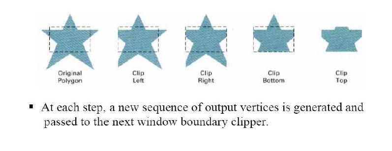
29 UNIT 2 Area Clipping/ Sutherland-Hodgman Polygon Clipping Unit-02/Lecture-07 Area Clipping- Similarly to lines, areas must be clipped to a window boundary Consideration must be taken as to which portions of the area must be clipped.

30 Sutherland-Hodgman Polygon C-

31

32 Sutherland-Hodgman Polygon Clipping Example- Start at the left boundary 1,2 (out,out) _ clip 2,3 (in,out) _ save 1, 3 3,4 (in,in) _ save 4 4,5 (in,in) _ save 5 5,6 (in,out) _ save 5 Saved points _ 1,3,4,5,5 6,1 (out,out) _ clip Using these points we repeat the process For the next boundary. S.NO RGPV QUESTIONS Year Marks Q.1 Draw a flowchart, illuminating the logic of the Sutherland Hodgeman algorithm. Q.2 Explain the Sutherland-Hodgeman polygon clipping algorithm with an example. 2012,

33 UNIT 2 Weiler-Atherton algorithms Unit-02/Lecture-08 Weiler -Atherton Polygon Clipping- RGPV(2011) Here, the vertex-processing procedures for window boundaries are modified so that concave polygons are displayed correctly. This clipping procedure was developed as a method for identifying visible surfaces, and so it can be applied with arbitrary polygon-clipping regions. The basic idea in this algorithm is that instead of always proceeding around the polygon edges as vertices are processed, we sometimes want to follow the window boundaries. Which path we follow depends on the polygon-processing direction (clockwise or counterclockwise) and whether tile pair of polygon vertices Currently being processed represents an outside-to-inside pair or an inside- to-outside pair. For clockwise processing of polygon vertices, we use the following rules: For an outside-to-inside pair of vertices, follow the polygon boundary. For an inside-to-outside pair of vertices, follow the window boundary in a clockwise direction. In Fig. 6-25, the processing direction in the Weiler-Atherton algorithm and the resulting clipped polygon is shown for a rectangular clipping window. An improvement on the Weiler-Atherton algorithm is the Weiler algorithm, which applies constructive solid geometry ideas to clip an arbitrary polygon against any polygon clipping region. Figure 6-26 illustrates the general idea in this approach. For the two polygons in this figure, the correctly clipped polygons calculated as the intersection of the clipping polygon and the polygon object.

34 Other Polygon-Cli pping Algorithms-Various parametric line-clipping methods have also been adapted to polygon clipping. And they are particularly well suited for clipping against convex polygon-clipping windows. The Liang-Barsky Line Clipper, for example, can be extended to polygon clipping with a general approach similar to that of the Sutherland-Hodgeman method. Parametric line representations are used to process polygon edges in order around the polygon perimeter using region-testing procedures Similar to those used in line clipping. S.NO RGPV QUESTIONS Year Marks Q Derive the form of the transformation matrix for a reflection about an arbitrary line with equation y=mx+c. Q.2 Contrast the efficiency of Cohen-Sutherland and Cyrus-beck line clipping algorithms

35