Contributions to the Bayesian Approach to Multi-View Stereo

Transcription

1 Contributions to the Bayesian Approach to Multi-View Stereo Pau Gargallo I Piracés To cite this version: Pau Gargallo I Piracés. Contributions to the Bayesian Approach to Multi-View Stereo. Human- Computer Interaction [cs.hc]. Institut National Polytechnique de Grenoble - INPG, English. <tel > HAL Id: tel Submitted on 15 May 2008 HAL is a multi-disciplinary open access archive for the deposit and dissemination of scientific research documents, whether they are published or not. The documents may come from teaching and research institutions in France or abroad, or from public or private research centers. L archive ouverte pluridisciplinaire HAL, est destinée au dépôt et à la diffusion de documents scientifiques de niveau recherche, publiés ou non, émanant des établissements d enseignement et de recherche français ou étrangers, des laboratoires publics ou privés.

2 INSTITUT NATIONAL POLYTECHNIQUE DE GRENOBLE THÈSE pour obtenir le grade de DOCTEUR DE L INPG N o attribué par la bibliothèque Spécialité : Imagerie, Vision et Robotique préparée au laboratoire GRAVIR dans le cadre de l Ecole Doctorale : Mathématiques, Sciences et Technologies de l Information, Informatique présentée et soutenue publiquement par Pau Gargallo i Piracés le 11 février 2008 Contributions à l approche bayésienne pour la stéréovision multi-vues Directeur de thèse : Peter Sturm Président : Rapporteurs : Examinateurs : JURY Augustin Lux Anders Heyden Renaud Keriven Marc Pollefeys Jean-Philippe Pons Emmanuel Prados Peter Sturm

3

4 Résumé La stéréovision multi-vues consiste à retrouver la forme des objets à partir de plusieurs images prises de différents points de vue connus. Ceci est un problème inverse où on cherche la cause (l objet) alors qu on observe l effet (les images). Sous une optique bayésienne, la solution serait une reconstruction qui reproduise au mieux les images observées tout en restant plausible a priori. Dans cette thèse, nous présentons des modèles et des méthodes permettant de minimiser la différence entre les images observées et les images obtenues par le rendu de la reconstruction. Pour ceci, il est nécessaire de tenir compte des occultations qui on lieu lors du rendu. Le résultat principal de la thése est le calcul de la dérivée de l erreur de reprojection par rapport aux variations de surface qui tiens en compte les changements de visibilité lors que la surface se déforme. Mots-Clés : Stérévision multi-vues, reconstruction de surfaces, inférence bayésienne, calcul variationnel, visibilité

5

6 Abstract Multi-view stereo is the problem of recovering the shape of objects from multiple images taken from different but known camera positions. It is an inverse problem where we want to find the cause (the object) given the effect (the images). From a Bayesian perspective, the solution would be the reconstruction that best reproduces the input images while at the same time being plausible a priori. Taking this approach, in this thesis we develop generative models and methods for computing reconstructions that minimize the difference between the observed images and the images sythetized from the reconstruction. Three models are presented. The first, represents the reconstructed scene by a set of depth maps. This gives high resolution results, but have problems at the objects boundaries. The second model represents the scene by a discreet occupancy grid, yielding to a combinatorial optimization problem, which is addressed through message passing techniques. The final model represents the scene by a smooth surface and the resulting optimization problem is solved via gradient descent surface evolution. In either model, the main difficulty is to correctly take into account the occlusions. Modeling self-occlusions results in optimization problems that challenge current optimization techniques. In this respect, the main result of the thesis is the computation of the derivative of the reprojection error with respect to surface variations taking into account the visibility changes that occur while the surface moves. This enables the use of gradient descent techniques, and leads to surface evolutions that place the contour generators of the surface to their correct location in the images without the need of additional silhouettes or apparent contours constraints. Keywords: Multi-view stereo, 3D reconstruction, Bayesian inference, variational calculus, visibility

7

8 Acknowledgements I would like to thank many people that helped be during all these years. Un Grand Merci pour toi Peter! Pour m avoir introduit dans le monde de la recherche en vision par ordinateur, et pour m avoir guidé et encouragé pendant tout ces années. C est en voyant que tu confiais en moi, plus de ce que je le fais moi même, que j ai trouvé les forces pour avancer. T as toujours été là quand j en ai eu besoin et tu m a laisser aller ailleurs quand j en ai eu envie. Thank you Anders Heyden and Renaud Keriven for having accepted to review this work and comment it, and thank you Marc Pollefeys, Jean-Philippe Pons and Emmanuel Prados for examining it. It is a privilege for me. Merci Augustin Lux d avoir accepté de présider la soutenance, et d avoir suivi avec intérêt le destin de tous ces étudiants du master IVR. Merci encore Manu pour toute l aide que tu m as offert, pour tous ces tableaux que nous avons rempli ensemble, et sur tout pour m avoir poussé à convertir les tableaux en articles, et les articles en une thèse. Merci encore aussi à toi Jean-Philippe pour avoir gentiment voulu partager ta magnifique librairie de level sets, qui m a été extrêmement utile. Thank you Kuk-Jin, merci Amaël i gràcies Sergi for the fruitful collaboration of the last months, and best wishes for the following. Thanks to all the current and former members of the MOVI team (now PER- CEPTION) for the friendly international environment. Thank you Daniel for all these endless conversations about research, software, art and the meaning of life. Et merci Anne d avoir géré magiquement pour moi toutes ces ordres de mission que je n ai jamais compris. Merci à vous les colocs du château pour les pâtes pesto. Et à Céline, Sergi, Hélène, Thomas, Helena et Yom pour ce dernières colocs et bureaux improvisées. I a tu, Alba, gràcies per tota la resta.

9

10 Résumé en Français Introduction Dans cette thèse nous nous intéressons au problème de la stéréovision multivues qui consiste à retrouver la forme d objets à partir d images. Étant données plusieurs images d un objet prises de différents points de vue connus, le but est de reconstruire la géométrie et, facultativement, l apparence de l objet. Ceci est l un des problèmes principaux de la vision par ordinateur, et ses applications sont nombreuses. Beaucoup d animaux, humains inclus, utilisent leurs yeux pour percevoir leur environnement. Que ce soit par l utilisation de deux yeux, ou en bougeant la tête, les animaux sont capables d estimer la profondeur et la géométrie des objets qui les entourent. Plusieurs sources d information comme la parallaxe, les ombres, la couleur ou les contours d occultation sont utilisées dans ce processus. Bien que ceci soit fait sans effort apparent par les animaux, on a pas encore réussi à le faire faire aux ordinateurs. Depuis le début des recherches en vision par ordinateur, les chercheurs ont développé des algorithmes pour extraire des informations tridimensionnelles à partir d images. Il n y a pas encore un algorithme général pour tout faire en toute situation, mais plusieurs sous-problèmes ont été résolus. Actuellement, le problème général de la reconstruction d objets à partir d images est résolu par étapes, la dernière desquelles étant celle qui nous intéresse. Les trois étapes principales sont : 1. Appariement parcimonieux : Dans une première étape, un certain nombre de points d intérêt, comme des coins ou des contours, sont détectés dans chaque image, et ensuite, mis en correspondance entre les différentes images. 2. Reconstruction parcimonieuse : La deuxième étape, consiste à utiliser les correspondances pour retrouver aussi bien le mouvement de la caméra que la position 3D des points d intérêt. 3. Stéréovision multi-vues : Finalement, en connaissant la position des caméras, 9

11 10 on calcule une reconstruction dense de la géométrie des objets apparaissant dans les images. Étant donné que les positions des caméras sont connues, la stéréovision multivues correspond à un problème d appariement dense d images. En effet, si on connaît la position des caméras et on sait qu un pixel d une image correspond à un certain pixel d une autre image, on peut retrouver la position 3D de ce point par triangulation. Malheureusement, il n est pas facile de mettre en correspondance les pixels d une image avec les pixels d une autre, car l apparence des objets peut changer d une image à l autre, il peut y avoir des ambiguïtés dans les zones peu texturées et certaines parties d une image peuvent être occultées dans l autre image. Dans cette thèse, nous n abordons pas le problème des changements d apparence. Nous partons de l hypothèse qu un point d un objet apparaît de la même couleur dans toutes les images où il est visible. Même avec cette hypothèse, il nous restent les problèmes des ambiguïtés et les occultations. Dans les parties uniformes des images, où plusieurs pixels ont la même couleur, la mise en correspondance devient impossible et il nous faudra ajouter des connaissances a priori si on veut donner une solution unique au problème. De plus, si une partie d un objet est visible dans une image et pas dans l autre, il ne sera pas possible de trouver des correspondances pour les pixels de la première image. Pour aborder ces difficultés, dans cette thèse, nous regardons la stéréovision multi-vues comme un problème inverse et nous adoptons l approche bayésienne. Nous commençons par décrire comment ont été obtenues les images à partir du monde qu on veut reconstruire et ensuite, nous utilisons l inférence bayésienne pour invertir ce processus et inférer la géométrie du monde à partir des images. Modèle de formation d images Les images sont le résultat d un processus complexe dans lequel la lumière émise par des sources lumineuses voyage dans l espace et arrive au capteur de la caméra après avoir été réfléchie par plusieurs objets. En graphisme, le rendu photo-réaliste s intéresse à la reproduction de ce phénomène et à la génération d images à partir d une description de la géométrie et de l apparence des objets. Ceci est un problème difficile, surtout dû aux multiples réflections qu un rayon de lumière subit avant d arriver à la caméra. On remarque tout de même que le problème est bien posé dans le sens où la solution (les images) est déterminée par l entrée (la géométrie et l apparence). On dit que c est un problème directe. La stéréovision multi-vues est le problème opposé où on connait les images et on recherche la forme des objets. On dit que c est un problème inverse car on

12 11 connait la conséquence et on cherche la cause. Sans autres informations, le problème est extrêmement difficile car l espace de recherche (toutes les formes et apparences des formes) est énorme, et la relation entre les images et les objets est complexe. Cette dernière difficulté est spécialement due aux inter-réflections qui font que la couleur observée dans un pixel dépend non seulement de l objet qui est visible dans le pixel, mais aussi de tout son environnement et du point de vue. Pour simplifier le problème et le rendre plus abordable, nous supposons dans cette thèse que la couleur apparente des objets ne dépend pas du point de vue. C est-à-dire qu un point de la surface d un objet apparaît de la même couleur dans toutes les images dans lesquelles il est visible. L apparence de chaque point de la surface des objets peut donc être décrite par une couleur et il n y a pas besoin de tenir compte des inter-réflections. Le modèle de formation d images qui est utilisé dans cette thèse est le suivant : étant donnée la géométrie des objets et la couleur de chaque point de la surface, la couleur observée dans un pixel correspond directement à la couleur du premier point de la surface qui intersecte le rayon de vue du pixel. Avec ce modèle de formation d images simplifié, il n y a plus d inter-réflections à tenir en compte car la couleur d un pixel dépend uniquement de la couleur du point observé. Cependant, il reste toujours une interdépendance entre les différents points de la surface des objets parce que pour trouver la première intersection de la surface avec le rayon de vue du pixel il faut connaître toute la surface. Autrement dit, pour savoir si un point de la surface est visible, il faut connaître tout la surface. Gérer correctement la visibilité est alors la difficulté principale qui reste. Approche bayésienne pour la stéréovision multi-vues Telle qu on l a présentée, la stéréovision multi-vues est le problème inverse du rendu. La théorie des probabilités est un outil mathématique idéal pour formaliser les problèmes inverses. Pour ce faire, il faut modéliser l ensemble des observations possibles et les variables inconnues dans un seul espace de probabilité. Avec un tel espace, on se pose la question : Quelle est la probabilité d une certaine solution étant données les observations? Formaliser des problèmes réels de cette façon est souvent appelé l approche bayésienne. Pour la stéréovision multi-vues les variables observées sont les valeurs des pixels des images d entrée, qu on notera I. Les variables inconnues sont la géométrie et la couleur du monde observé, qu on notera w. La distribution de probabilité conjointe des images et du monde, p(i, w), est une distribution sur l énorme espace de toutes les images et mondes possibles. Cette distribution doit

13 12 contenir toutes nos connaissances du problème : Pour chaque paire d un ensemble d images et d un monde, combien nous paraît-il plausible que cette paire existe? Définir une distribution de probabilités qui représente exactement nos connaissances sur le problème est une tâche difficile. Cependant, on peut obtenir des approximations satisfaisantes d une manière naturelle, en décomposant la distribution conjointe en quelques termes plus simples. La relation cause à effet qui existe entre le monde et les images fait qu il est intuitif de décomposer la probabilité conjointe comme ceci : p(i,w) = p(i w)p(w). (1) Les deux termes de la décomposition sont les suivants : Le premier terme, p(i w), est la probabilité conditionnelle des images observées étant donné un monde hypothétique. Cette distribution est appelée la vraisemblance et doit répondre à la question : Si w était le monde réel, quelle serait la plausibilité d observer les images I? Par exemple, si le monde contient des objets verts, on espère que les images vont être, elles aussi, vertes et on dira que observer du rouge dans un monde vert n est pas vraisemblable. Plus précisément, si on nous donne un monde w on peut le photographier (par rendu) depuis les mêmes points de vue que les images d entrée. Le résultat est un ensemble d images I (w) qu on appelle images idéales et qui correspondent aux images que, en principe, on devrait observer si le monde était w. En comparant les images idéales avec les images observées, on peut alors facilement définir sa vraisemblance. Cette mesure de similarité entre les image idéales et les images observées sera appelée l erreur de reprojection. La minimisation de l erreur de reprojection est le problème principal considéré dans cette thèse. Le deuxième terme, p(w), est la distribution a priori sur l espace des mondes possibles. On l appelle a priori parce qu elle doit être définie avant de tenir compte des observations. Elle doit répondre à la question : Quelle est la plausibilité que le monde réel soit w? En effet, même avant d observer les images, on a déjà une idée sur à quoi le monde ressemble. On sait par exemple que la matière est souvent regroupée dans des objets solides et non pas aléatoirement repartie dans l espace. On sait aussi que les objets ont des couleurs caractéristiques et qu ils ne sont pas texturés par des couleurs aléatoires. Toutes ces connaissances doivent être représentées par la distribution a priori. Cette décomposition est naturelle parce qu elle suit l ordre logique qu il faut suivre pour générer des images à partir de rien. Il faut d abord créer un monde ;

14 13 Figure 1: Modèle génératif pour la stéréovision multi-vues. D abord on crée le monde, ensuite on en prend des photos. le choix de ce monde est guidé par la distribution a priori p(w). Ensuite, il faut photographier le monde ; comment prendre des photos est encodé dans la vraisemblance p(i w) (voir Figure 1). Ces types de décomposition sont appelés modèles génératifs ; ils sont le modèle idéal pour formaliser des problèmes inverses. Une fois que la distribution conjointe est définie, on peut répondre à toute question concernant les variables modélisées. Dans notre cas, il est naturel de se poser la question : Quelle est la probabilité du monde étant données les images? La réponse à cette question est la distribution a posteriori p(w I). Elle peut être déterminée à partir de la distribution conjointe par la relation p(w I) = p(i,w) p(i) = p(i w) p(w) p(i w) p(w) dw. (2) Cette équation est souvent appelée la règle de Bayes. Elle est particulièrement intéressante parce qu elle met en relation ce qu on veut connaître, la distribution a posteriori, avec ce qu on connaît, la vraisemblance et l a priori. Dans quelques applications, calculer une distribution de probabilité sur toutes les solutions possibles ne sera pas un résultat satisfaisant et il est préférable d en choisir une seule un bon monde. Pour ceci il est raisonnable de choisir le monde le plus probable. Ceci est appelé le maximum a posteriori (MAP). En résumé, l approche bayésienne pour la stéréovision multi-vues consiste en trois étapes : 1. Choisir l espace des mondes (ou reconstructions) possibles et une distribution a priori p(w), 2. décrire le processus de formation d images en spécifiant la vraisemblance p(i w), 3. et, finalement, calculer ou maximiser la distribution a posteriori p(w I).

15 14 Autres approches Le stéréovision a été étudiée depuis bien longtemps. Il n est donc pas surprenant qu il existe plusieurs différentes approches au problème. Nous pouvons les classifier grossièrement en trois types : Les méthodes directes, les méthodes de minimisation d énergie et les hybrides. Méthodes directes On dit qu un point de l espace est photo-cohérent s il apparaît de la même couleur dans toutes les images. En général, les points qui appartiennent à la surface des objets sont photo-cohérents. Ceci suggère un algorithme très simple pour reconstruire la surface des objets : On peut parcourir tout l espace et pour chaque point regarder si le point est photo-cohérent ou pas ; s il l est, on l accepte comme étant un point de la surface. Un tel algorithme ne marche pas toujours pour deux raisons. D un côté, le fait que les points de la surface sont photo-cohérents n implique pas que tous les points photo-cohérents sont sur la surface. De l autre côté, à cause des occultations, pas tous les points de la surface sont photo-cohérents dans toutes les images. L algorithme va donc à la fois détecter quelques faux points et ne pas détecter tous les bons. Malgré tout, ce simple algorithme est la base des méthodes directes. Pour réduire le nombre de fausses détections il est fréquent de demander que non seulement le point soit photo-cohérent mais aussi un certain voisinage [129]. Pour augmenter le nombre de bonnes détections il faut gérer les occultations. La façon la plus simple est d utiliser des critères de photo-cohérence robustes [149, 150, 76, 74]. La façon dans laquelle l espace est parcouru est aussi un facteur important. Les deux stratégies majeures sont de chercher la profondeur de chaque pixel d une image de référence [75, 27], ou bien d explorer une grille régulière de voxels [131, 58]. En général les performances des méthodes directes restent limitées du fait qu elles prennent des décisions dures sur une partie de la scène sans en connaître le reste et qu il est difficile d introduire des informations a priori comme par exemple la préférence pour les surfaces lisses. Méthodes de minimisation d énergie Les problèmes rencontrés par les méthodes directes peuvent être résolus en considérant le problème d une façon globale. Au lieu de prendre des décisions indépendantes pour chaque point de l espace, on peut chercher la surface à reconstruire comme un tout. Pour ceci on définit un coût, ou énergie, pour chaque surface possible, et

16 15 on cherche la surface qui le minimise. Le plus souvent, cette énergie est formée par deux termes, un qui correspond à la vraisemblance et qui assure que la surface sera cohérente avec les images et l autre qui correspond à l a priori et qui force la surface à avoir une forme raisonnable. On peut distinguer deux types d approches pour la définition d une telle énergie : Approches génératives et non-génératives. Approches non-génératives Celles-ci sont l extension logique des méthodes directes. Les méthodes directes utilisent un critère de photo-cohérence pour décider si un point est sur la surface ou pas. Si l on dispose d une surface candidate, on peut mesurer sa qualité en faisant la somme de ce critère sur tous les points de la surface. On a défini ainsi un critère de photo-cohérence global pour toute la surface. Une façon pratique de représenter la surface est d utiliser une carte de profondeurs par rapport à une image de référence. Pour chaque pixel de l image de référence on calcule sa profondeur. Le critère de photo-cohérence est alors la somme sur tous les pixels de l image de référence de la photo-cohérence du point 3D associé [129, 125, 164, 148, 159, 3, 146]. Des variables de visibilité additionnelles peuvent être utilisées pour mieux tenir compte des occultations [8, 76, 147]. Si on veut reconstruire toute la surface visible dans les images en utilisant des cartes de profondeurs, il faudra en calculer une pour chaque image d entrée [80, 115, 86]. Une autre façon de reconstruire toute la surface est de la représenter de façon indépendante des images par une surface quelconque. Dans ce cas, la surface optimale peut être calculée par évolution de surface, utilisant une représentation par ensembles de niveaux [41, 70, 135, 72], des maillages [46, 187, 60] ou des particules orientées [45, 153]. Il est aussi possible [16] d utiliser la méthode de graph-cuts pour minimiser ce type d énergies [111, 166, 185, 67, 161]. Un problème récurrent de ce type d énergies est la tendance des surfaces à diminuer ou disparaître. En effet, plus la surface est petite, plus petit sera le coût de photo-cohérence (car on le somme sur une surface plus petite). Ceci est appelé la distorsion systématique vers les surfaces minimales [5, 179]. Pour répondre à cet effet, il a été proposé d utiliser des forces de gonflage [168, 166, 61, 5, 179]. Approches génératives Une façon alternative de définir une énergie à minimiser est de suivre l approche bayésienne telle qu on l a présentée dans la section précédente [25, 105, 177, 73, 71, 118, 79]. Dans ce cas, l énergie correspond au négatif du logarithme de la probabilité a posteriori de la surface. Ceci est la somme d une énergie de vraisemblance plus une d a priori. L énergie de la vraisemblance correspond à l erreur de reprojection qui mesure la différence entre les images

17 16 observées et les images reproduites à partir de la reconstruction. Une difficulté importante avec cette approche est que l erreur de reprojection contient des termes de visibilité qui sont difficiles à minimiser correctement. Des solutions partielles ne fonctionnant que sur des surfaces convexes ont été trouvées [177]. Dans le dernier chapitre de cette thèse (chapitre 4), nous montrons comment l erreur de reprojection peut être minimisée de façon exacte par évolution de surfaces [50]. Strecha et d autres ont développé des modèles génératifs qui utilisent une seule carte de profondeurs [144, 145, 143]. Pour pouvoir gérer les occultations et d autres effets, ils définissent un processus marginal qui est chargé de la génération des pixels qui observent ces effets. Nous avons développé une extension de ce modèle qui utilise plusieurs cartes de profondeurs [51]. Ceci permet à la fois de modéliser toute la scène et de tenir compte des occultations de façon géométrique (chapitre 3). Méthodes hybrides Finalement, un troisième groupe de méthodes utilise à la fois des méthodes directes et de minimisation d énergie. L idée est de faire la reconstruction en deux étapes. Dans la première, une méthode directe est utilisée pour trouver un nuage de points sur la surface. Normalement, ce nuage sera bruité et contiendra des points qui ne sont pas vraiment sur la surface. Dans une deuxième étape, une méthode de minimisation d énergie est utilisée pour caler une surface sur le nuage de points de façon robuste [94, 48, 60]. Une méthode alternative est de calculer des cartes de profondeurs avec une méthode directe, et de les combiner avec une méthode de minimisation d énergie [31, 63, 172, 141, 181, 100]. Ces approches combinent la vitesse et la simplicité des approches directes avec la précision et la robustesse des méthodes de minimisation d énergie. Contributions de cette thèse Dans cette thèse, nous utilisons systématiquement l approche bayésienne décrite précédemment. Nous appliquons cette approche à trois représentations différentes de la géométrie du monde, et nous étudions les problèmes algorithmiques qui en découlent. Nous commençons par étudier le cas où le monde est représenté par un ensemble de cartes de profondeurs (chapitre 3). L utilisation de plusieurs cartes de profondeurs est aussi bien motivée par la haute résolution que cette représentation offre que par le fait qu en cherchant la profondeur de

18 17 chaque pixel d entrée on est sûr de tout modéliser. En pratique on observe deux difficultés liées à cette représentation. Premièrement, les contours d occultation sont difficiles à optimiser car de petits déplacements de ceux-ci nécessitent de grandes variations des profondeurs des pixels voisins. Deuxièmement, la représentation est redondante, ce qui impose l ajout de contraintes supplémentaires pour imposer la cohérence entre les différentes cartes de profondeurs. Au vu de cela, nous avons développé un modèle dans lequel le monde est représenté de façon indépendante des images par une fonction d occupation de l espace. Le calcul des cartes de profondeurs est tout de même requis par le processus de formation d images, parce qu elles déterminent les parties visibles de la surface. Dans notre modèle, comme dans la réalité, les cartes de profondeurs sont déterminées à partir de la fonction d occupation. Dans le chapitre 4, nous traitons la version discrète du modèle, où l on considère la fonction d occupation d une grille de voxels. Ceci induit un problème d optimisation combinatoire important, que nous représentons sous la forme d un graphe de facteurs. Finalement, dans le chapitre 5, nous traitons la version continue du modèle d occupation, où l on considère l occupation de tous les points de l espace. Dans ce cas, la recherche du maximum a posteriori du modèle devient un problème d optimisation de formes. Nous résolvons ce problème par une descente de gradient. Le calcul du gradient de la vraisemblance est la contribution principale de cette thèse. Le calcul est intéressant parce qu il caractérise les changements de visibilité qui apparaissent lorsqu on déforme une surface. En résumé, du côté qu est-ce qu il faut optimiser, nous proposons le modèle d occupation, combiné avec des cartes de profondeurs, parce qu il explique de manière naturelle le processus de formation d images, notamment les occultations. Du côté comment l optimiser, nous calculons la dérivée de l erreur de reprojection ce qui permet d optimiser le modèle par des méthodes de déformation de surface. Représentation utilisant plusieurs cartes de profondeurs Quand on veut reconstruire une scène à partir d images, on peut utiliser plusieurs représentations (principalement des voxels, des fonctions implicites ou des maillages). Quelque soit la représentation utilisée, si on veut calculer la visibilité de

19 18 façon géométrique, il est fort probable qu on ait besoin de calculer des cartes de profondeurs, car elles déterminent les parties visibles de la scène. La question qu on considère dans ce chapitre est : Serait-il possible d utiliser les cartes de profondeurs elles-mêmes comme représentation de la géométrie, au lieu de les calculer à partir d une autre représentation? La motivation principale pour utiliser des cartes de profondeurs est leur haute résolution. Les images numériques contiennent des millions de pixels. Si on veut utiliser un modèle génératif pour reconstruire une scène à partir d images, il faut que le modèle soit capable d expliquer chacun de leurs pixels. La résolution de la reconstruction doit donc être en accord avec la résolution des images. Bien qu il soit possible de construire des grilles de voxels parcimonieuses ou des maillages gigantesques, les cartes de profondeurs sont une solution plus simple sur le plan algorithmique. Les reconstructions impressionnantes obtenues par Strecha et al. [146, 144] en utilisant des cartes de profondeurs sont un bon exemple de résultats qu il serait difficile d obtenir avec d autres représentations. Afin de modéliser complètement la scène qui apparaît dans les images, nous développons dans ce chapitre un modèle génératif qui utilise une carte de profondeurs pour chaque image, de sorte que tous les pixels soit expliqués. La profondeur d un pixel correspond à la profondeur du point 3D visible dans ce pixel. Ces points 3D forment un nuage de points, et ce nuage est ce qu on utilise comme représentation de la géométrie de la scène. L apparence des objets sera représentée par la couleur des points. Pour pouvoir inférer les profondeurs et les couleurs, nous définissons la probabilité conjointe des images, des profondeurs et des couleurs suivant l approche bayésienne décrite précédemment. Pour bien tenir compte des occultations géométriques, nous introduisons des variables de visibilité qui indiquent quels points du nuage sont visibles dans quelle image. Ces variables de visibilité dépendent directement des profondeurs pour pouvoir les déterminer de façon géométrique. Cependant, la dépendance n est pas stricte car un point géométriquement visible peut être occulté par un effet comme un reflet spéculaire ou un objet mobile qui n est pas modélisé. Une attention particulière est portée à la définition d un a priori sur l ensemble des cartes de profondeurs. Idéalement, elles devraient être cohérentes les unes avec les autres et former une seule surface. De plus, on voudrait qu elles soient lisses partout sauf le long des contours d occultation où de grandes discontinuités doivent être autorisées. La reconstruction est faite par maximisation de la probabilité a posteriori des profondeurs et des couleurs. Les variables de visibilité restent cachées et doivent être marginalisées. Pour ceci, on utilise l algorithme EM (Expectation Maximization) qui alterne entre l estimation des probabilités des variables de visibilité, et la maximisation de l a posteriori.

20 19 Résultats Nous avons testé la méthode avec quelques jeux d images. Pour les cas simples, où il n y a pas d occultations elle marche bien et les résultats sont de très haute résolution. Pour des cas plus compliqués dans lesquels un objet se trouve devant un fond distant on a trouvé des difficultés liés aux contours d occultation. Le problème est que pour bien placer les contours d occultation il faut que les valeurs de profondeur des pixels voisins changent de façon non continue ; or la méthode d optimisation que nous utilisons ne permet pas ce type de changements. Une heuristique a été développée pour palier ce problème. Les figures 2 et 3 montrent un jeux d images difficile, avec les cartes de visibilité estimées, l évolution de l algorithme et le résultat final. Conclusion L utilisation de plusieurs cartes de profondeurs a montré quelques avantages, notamment, la haute résolutions des résultats et la possibilité de gérer les occultations de façon géométrique. Cependant, elle a aussi montré deux inconvénients importants. Premièrement, il a fallu concevoir un a priori ad hoc qui force les différentes cartes de profondeurs à être cohérentes. Ceci n est pas très naturel car dans le monde réel les cartes de profondeurs sont toujours cohérentes, puisqu elles sont issues d une même géométrie. Deuxièmement, nous avons rencontré des problèmes aux contours d occultation. En effet, notre a priori permet d obtenir des discontinuités dans les cartes de profondeurs. Cependant, notre méthode d optimisation ne permet pas de placer ces discontinuités à la position correcte. Les prochains chapitres adresserons ces problèmes en utilisant une représentation de la géométrie indépendante des images et non redondante. Représentation utilisant l occupation et la profondeur Dans ce chapitre, nous développons un modèle génératif pour la stéréovision multi-vues, dans lequel la géométrie des objets est définie par une fonction d occupation discrète. Dans ce modèle, le monde est représenté par une division de l espace en régions pleines de matière ou vides. La profondeur d un pixel est alors déterminée de façon naturelle comme étant la profondeur du premier point occupé sur son rayon de vue. Connaissant donc la profondeur, la couleur du pixel correspond à la couleur de ce point 3D. Ce modèle simple a deux avantages. Premièrement, par rapport à d autres modèles qui utilisent des fonctions d occupation, celui-ci modélise explicitement la relation déterministe qui existe entre l occupation et la profondeur. Ceci per-

21 20 Figure 2: Staty : En haut, les cinq images d entrée. En bas, les cartes de visibilité estimées, i.e. la probabilité que les points 3D correspondants à la carte de profondeurs d une image, soient visibles dans une autre image.

22 Figure 3: Staty : A gauche, un rendu à base des points de l évolution de la reconstruction pendant l optimisation. A droite, deux rendus de la carte de profondeurs estimée pour la deuxième image. 21

23 22 Figure 4: Réseau bayésien associé à un seul pixel et son rayon de vue. L occupation des voxels u i détermine la profondeur d. La couleur du pixel I correspond à la couleur C à la profondeur d. Figure 5: Graphe de facteurs correspondant au modèle pour un seul pixel (gauche) et pour deux pixels (droite). met de gérer les occultations de façon exacte. Deuxièmement, à la différence des méthodes qui utilisent des cartes de profondeurs, le fait de déterminer la profondeur à partir de la fonction d occupation fait que les différentes cartes de profondeurs soient automatiquement cohérentes. Dans ce chapitre, nous explorons la version discrète de ce modèle, dans laquelle l espace est divisé en un nombre discret de cellules (ou voxels) qui peuvent être pleines ou vides. La figure 4 montre le réseau bayésien associe à un seul pixel. L occupation de tous les voxels sur son rayon de vue est utilisée pour déterminer la profondeur du pixel. Cette profondeur et la couleur de l espace sont alors utilisées pour déterminer la couleur du pixel. Quand la couleur de l espace est connue, ce modèle peut être représenté par le graphe de facteurs apparaissant dans la figure 5. Dans ce graphe, la vraisemblance de chaque pixel correspond à un gros facteur qui lie tous les voxels sur son rayon de vue. L optimisation de cet énorme graphe de facteurs est un problème combinatoire très complexe. Nous avons développé les règles de passage de messages permettant d optimiser le graphe par propagation de croyances (en anglais : be-

24 23 Figure 6: Résultats d une expérience avec un seul pixel. lief propagation). La taille des facteurs et le grand nombre de boucles limitent la précision des résultats obtenus par cette méthode. Résultats Nous avons validé le modèle en faisant différentes expériences. La première, consiste à optimiser un modèle réduit qui contient un seul pixel. Pour ceci, la vraisemblance de la profondeur du pixel a été fixée manuellement (ligne bleue, figure 6). Le vrai a posteriori sur l occupation qui résulte de cette vraisemblance a été calculé par des méthodes d échantillonnage (ligne verte). Quand on calcule cet a posteriori par la méthode de passage de messages, on obtient un résultat assez différent (ligne rouge). En général, pour différentes vraisemblances, le vrai a posteriori et celui calculé par le passage de messages sont toujours similaires dans les voxels les plus proches du point de vue, et de plus en plus différents lorsqu on s en éloigne. Nous avons aussi calculé le maximum a posteriori (l occupation la plus probable, ligne bleue claire) avec la méthode de passage de messages. Le vrai maximum serait la configuration dans laquelle tous les voxels avant le pic de la vraisemblance (voxel 32) sont vides et tous les autres sont pleins. On observe, que le résultat obtenu est vide pour trop de voxels. Nous avons alors testé la méthode pour des paires stéréo en espérant que l interaction entre les différents pixels pourrait améliorer les résultats. En effet, les résultats sont meilleurs (figure 7), mais on observe toujours cet effet de surcreusage. Ceci est évident dans les zones moins texturées, où des gros trous

25 24 Figure 7: L image de gauche, la vérité terrain et nos résultats.

26 25 apparaissent. Conclusion Nous avons développé un modèle qui explique les images d entrée à partir de l occupation de l espace par le moyen des profondeurs des pixels. Le modèle est très satisfaisant car il correspond à la façon de laquelle les images ont été générées et modélise les occultations explicitement. Cependant, l optimisation du modèle s est révélée bien difficile. La méthode de passage de messages que nous avons utilisée n a pas fonctionné correctement ce qui est normal car le graphe contient beaucoup de boucles. On a donc un bon modèle, mais qui est, à présent, trop compliqué à optimiser. Le gradient de l erreur de reprojection Dans ce chapitre nous développons un modèle génératif pour la stéréovision multivues qui représente la géométrie de la scène par une surface fermée et lisse. Ce modèle peut être vu comme étant la version continue du modèle d occupation + profondeurs du chapitre précédent. Cette fois-ci, on considère l occupation de tous les points de l espace et non seulement de quelques cellules. La frontière entre les points occupés et ceux vides est la surface qu on cherche à optimiser. Dans ce modèle, la vraisemblance des images est calculée en projetant la surface reconstruite dans les images et en comparant les images prédites avec celles observées. L énergie correspondante à cette vraisemblance est une intégrale sur le domaine de l image de la différence entre les deux images. Nous appelons ce type d énergies, fonctionnelles d erreur de reprojection. Notre contribution principale est le calcul exacte de la dérivée de la fonctionnelle d erreur de reprojection. Ceci permet, pour la première fois, d optimiser ce type de fonctionnelles par des méthodes d évolution de surfaces. La principale difficulté a été de bien tenir compte des changements de visibilité qui apparaissent lorsqu on déforme la surface. Nous présentons une étude géométrique et analytique de ces changements qui est fortement basée sur la théorie des distributions. Cette étude est ensuite utilisée pour calculer la dérivée de la fonctionnelle. Notre analyse montre et quantifie la forte influence qu a le mouvement des contours d occultation sur l erreur de reprojection. Comme conséquence de cette forte influence, pendant la minimisation de l erreur de reprojection, on observe que les contours d occultation ont tendance à se placer dans leur position correcte. Notre travail permet donc de justifier les méthodes qui utilisent des contraintes de silhouettes ou de contours apparents et de les comprendre comme étant des approximations d un seul critère : l erreur de reprojection.

27 26 Figure 8: Les quatre images d entrée et trois rendus de la reconstruction obtenue. Résultats Nous avons réalisé des évolutions de surfaces pour des jeux d images de synthèse et réelles. Les images des boules (figure 8), par exemple, ont été conçues pour montrer la tendance des contours d occultation à bien se placer au cours de l évolution de surface. En effet, les images ne contiennent aucune texture, donc, la seule information présente sont les contours d occultation. Les résultats montrent les trois boules parfaitement séparées. Les évolutions sur des images réelles comme celles du temple (figure 9) montrent la capacité des évolutions de grossir, ce qui était difficile à obtenir avec les méthodes d évolution de surface précédentes. Conclusions Dans cette thèse, nous avons abordé le problème de la stéréovision multi-vues d un point de vue bayésien. Nous avons décrit comment les images peuvent être générées à partir d un modèle, et nous avons ensuite utilisé l inférence bayésienne pour invertir ce processus et retrouver le modèle à partir des images. La relation entre le modèle et les images est particulièrement compliquée à cause des occultations qui apparaissent pendant le processus de formation d images. De plus l espace des formes dans lequel il faut faire de l inférence est aussi très complexe. L inférence est donc difficile. Nous avons développé trois modèles utilisant différentes représentations de la forme des objets. Un premier utilisant des cartes de profondeurs, un deuxième utilisant l occupation d une discrétisation de l espace, et un troisième utilisant des

28 Figure 9: Première ligne : Quelques images du temple. Deuxième ligne : L évolution de la surface. Troisième ligne : La reconstruction finale. Dernière ligne : La reconstruction finale pour le dinosaure. 27

29 28 surfaces lisses. En regardant les choses a posteriori, je pense que le fait d avoir exploré des représentations de formes spécifiques n a pas été très bénéfique et que ceci a retardé la compréhension du problème fondamental qui est la minimisation de l erreur de repojection. Ce problème apparaît quelque soit la représentation utilisée. Le calcul de la dérivée de l erreur de reprojection est un premier pas pour résoudre ce problème. Le modèle d occupation discret est tout de même utile, puisqu il y a des situations où l approche d évolution de surfaces n est pas utilisable. De plus, bien qu il n y ait pas encore une bonne méthode pour l optimiser, avoir une version discrète du même problème devrait permettre d explorer des méthodes qui ne sont pas utilisables pour le modèle continu. En ce qui concerne des travaux futurs, il y a deux directions parallèles dans lesquelles on peut avancer : Chercher des meilleures méthodes d optimisation pour les modèles présentés, et concevoir de meilleurs modèles. Pour la version discrète du modèle d occupation il faut regarder si les méthodes de coupes de graphes (en anglais : graph-cuts) seraient applicables, car il a été montré qu elles sont plus performantes que le passage de messages pour des graphes avec beaucoup de boucles [83]. Pour la version continue, il faut explorer la possibilité de développer des méthodes de relaxation convexe. Ces méthodes ont été récemment utilisées pour d autres problèmes variationnels avec un grand succès [108, 18]. Finalement, de meilleurs modèles qui représentent mieux le monde réel devraient être conçus. Il est facile de décrire des modèles plus compliqués il suffit de décrire la façon dont les images sont générées. Cependant, ceci amène à des modèles bien plus compliqués à optimiser que ce que nous avons présenté ici. Un équilibre entre la complexité du modèle et la facilité avec laquelle on peut l optimiser doit être trouvé.

30 INSTITUT NATIONAL POLYTECHNIQUE DE GRENOBLE PhD Thesis for obtaining the title of DOCTOR OF THE INPG Specialized in Computer Graphics, Computer Vision and Robotics Prepared at GRAVIR laboratory and the graduate school of Mathématiques, Sciences et Technologies de l Information, Informatique presented by Pau Gargallo i Piracés the 11th February 2008 Contributions to the Bayesian Approach to Multi-View Stereo Advisor: Peter Sturm President: Reviewers: Examiner: JURY Augustin Lux Anders Heyden Renaud Keriven Marc Pollefeys Jean-Philippe Pons Emmanuel Prados Peter Sturm

31

32 Contents 1 Introduction The Multi-View Stereo Problem The Image Formation Process Basic Setup and Notation Isotropic Radiance Model Bayesian Rationale for Multi-view Stereo World Prior Image Likelihood A Word on Evidence Conclusion Contributions of this Thesis State of the Art Approaches Bottom-Up: Direct Methods or Detectors Top-Down: Energy Minimization and Inference Hybrid Additional Cues Known Geometry and Visibility Constraints Photometric Cues Tools Shape Representations Optimization Methods Conclusion A Multiple Depth Maps Model Introduction Model Depth and Color Maps and Visibility Variables Decomposition Likelihood

33 32 CONTENTS Geometric Visibility Prior Multiple Depth Maps Prior Inference Experiments Conclusion The Occupancy Depth Model Introduction Model Occupancy, Depth and Color Variables Decomposition World Priors Pixel Likelihood Inference Factor Graph Representation Message Passing Color Estimation Experimental Validation Conclusion The Gradient of the Reprojection Error Introduction Related Work Mathematical Background and Notation Level Set and Characteristic Functions Functional Derivatives Understanding the Visibility Geometrical Description Mathematical Formulation Spatial Derivative of the Visibility Temporal Derivative of the Visibility Temporal Derivative of a Quantity Integrated over the Visible Volume Differential of the Reprojection Error Functional Case where g does not depend on the Normal With Normals Comparison with the Gradient of the Weighted Area Functional Applications Multi-view Stereo Surface Reconstruction from Range Images

34 CONTENTS Multi-view Normal Integration Implementation Experiments Synthetic Data Real Images Dealing with Non-Lambertian Effects Conclusion Conclusion Sumary Future Work Better algorithms Better models

35

36 Chapter 1 Introduction In this chapter we introduce the problem of multi-view stereo. The general problem being very complex, we concentrate on the special case of Lambertian scenes under fixed lighting. We describe the simple image formation process associated with these scenes. Then, we present the generative Bayesian approach to invert the process, which will drive the developments of this thesis. 1.1 The Multi-View Stereo Problem Multi-view stereo is the problem of recovering the shape of objects from images. Given a set of images of an object or a scene taken with different camera positions, the goal is to reconstruct the shape, and optionally the appearance, of the object. It is one of the central problems in computer vision and its applications are uncountable. Many animals, including humans, use their eyes to perceive the world. By observing the world from different viewpoints, either using two eyes or by moving the head, animals are able to perceive depth and to understand the threedimensional geometry of the world. Many cues, such as motion parallax, shading, color information or occlusion boundaries, are used in the process. While this ability does not seem to require any effort to animals, being able to reproduce it on computers has proved to be difficult. Since the beginning of computer vision, researchers have developped computational algorithms to extract 3D information from images. Although a general system that will work in any situation is still to be found, many partial problems have been solved. Currently, the standard pipeline for reconstructing objects from images has mainly three stages (Figure 1.1): 1. Sparse matching In a first stage, a number of interesting features, like small image patches, edges or corners, are detected on each image, and 35

37 36 Chapter 1: Introduction Figure 1.1: The 3D reconstruction pipeline: feature matching, structure from motion, and dense reconstruction. then matched between the different images. 2. Structure from motion In a second stage, the features correspondences are used to infer the camera position as well as the 3D position of the features [59]. 3. Multi-view stereo Finally, with the known camera positions a dense reconstruction of the geometry of the objects is computed. Given that the camera positions are known, the multi-view stereo problem is equivalent to the problem of finding dense correspondences between the pixels (or sub-pixels) in the different images. Indeed, if we know the camera positions and we know that two points in two images are the projection of the same 3D point, the position of this point can be found by triangulation. Unfortunately, finding dense correspondences between images is rather hard. The main difficulties are the changes of appearance, ambiguities and occlusions. When an image is taken, the light reflected or emitted by the objects of the scene is captured by a camera. To recover the geometry of the objects from the light captured by the camera, one has to understand the relationship between the object geometry and the captured light. In general, the problem is very hard because the light reflected by an object depends on the object itself, but also on its surroundings. The same object will appear differently under different lighting conditions. Moreover, the appearance of an object changes when the point of view

38 1.2 The Image Formation Process 37 changes because objects do not reflect the same light in all directions. In this thesis, we will not confront the problem of appearance changes, and we will assume that objects reflect the same light in all directions (see next section). Even with this simplifying assumption, we are left with the problems of ambiguity and occlusions. In uniform parts of the images, where many pixels have the same color, finding correspondences is a problem with ambiguous solutions, and one has to rely on prior knowledge if a single solution is desired. In addition, occlusions make the correspondence problem ill-defined. If a part of an object appears in an image, but is occluded in another, pixels of the first image will have no correspondent in the second. To tackle these problems, in this thesis, we adopt the Bayesian approach. We start by describing how the images have been generated from the unknown world, and then use Bayesian inference to reverse the process and infer the unknown world from the images. In the following section, we describe the image formation process and introduce some basic notation. Later, in section 1.3, we present the Bayesian approach to inverting the process. 1.2 The Image Formation Process In this section we overview the real image formation process, and then present the simplified version that will be used in this work. Images are the result of a complex physical process involving basically three factors: 1. the light, traveling all around being reflected, refracted, absorbed, scattered and diffracted; 2. the world geometry and reflectance properties that reflect, refract, absorb, scatter and diffract the light; 3. and the camera capturing the light arriving it its sensor. To get an idea of the complexity of the process, it is enough to imagine the life of one of the photons that is serving your eyes to read this text (see figure 1.2). If the blinds of your window are open, chances are that the photon s life started eight minutes ago in the sun. It has traversed the atmosphere, the clouds and the window; it has bounced against many walls; and then, finally, has hit this paper and has been projected into your retina. This is happening for zillions of photons at the same time, and each of them is taking its particular path from the sun to your eye. In order to describe how an image is formed exactly, it would be necessary to track all the photons that are susceptible of arriving at the camera. The state of

39 38 Chapter 1: Introduction Figure 1.2: The life of a photon from the sun to your eye through this paper and more. all the photons at an instant can be expressed compactly by counting the number of them that are traversing every point in every direction. The appropriate magnitude for this counting is radiance, and the function that gives the counting at every point in every direction is the plenoptic function [2]. For a point x and a direction v, the plenoptic function L(x, v) gives the amount of radiance traversing a differential patch in the direction v, when the patch is placed at x and is orthogonal to v. Humans and camera sensors are able to perceive colors. These means that photons of different wavelength are perceived differently. Thus, it is convenient to include the wavelength as parameter of the plenoptic function. In this case, L(λ,x,v) is radiance of wavelength λ traversing x in the direction v. Because the plenoptic function completely represents the state of the light (up to polarization), it determines everything that can be observed. Images are observations of the plenoptic function, and cameras are devices that perform these observations. Central cameras, for example, measure the plenoptic function at a single point but in many directions. Measuring in all the directions produces panoramic images. The plenoptic function is determined from the world geometry and reflectance properties that describe how the light is transmitted and reflected. Given a description of the world it is thus possible to compute the images that will be captured by a camera in that world. This is the goal of photo-realistic rendering in computer graphics. Of course, computing the whole plenoptic function is a huge computational challenge. Nevertheless, the problem is solvable in the sense that it has a well defined solution. We say that it is a direct problem because the output is a consequence of the input we know the cause and we seek the consequence.

40 1.2 The Image Formation Process 39 Multi-view stereo is exactly the opposite problem. We are given a set of images, and we want to find the world that generated them. We are not even given the whole plenoptic function, but only a small sampling. We say that it is an inverse problem because we are given the consequence and we want to find the cause. Without any further assumption, the problem is extremely difficult; it is ambiguous, the solution space (world geometry and reflectance properties) is huge, and the relationship between the images and the world is complex. The latter is specially due to the multiple reflections that a photon can experiment before arriving at the camera. The color observed at a pixel is not only due to the surface point visible on that pixel, but also to all the other surface points that are radiating light to that point. Hence, every pixel contains information about the whole surface, and it is difficult to split this information into independent pieces for each surface point. In order to simplify the problem we will do two things: Firstly, instead of searching the reflectance properties of the surface, we will directly search for the exitant radiance at the points in the surface of the world (i.e. the amount of light reflected by every surface point). This avoids the interreflection problem because the observed value in a pixel is directly and only related to the exitant radiance at the observed point. However, the problem is still ambiguous, even more than before, beause we are not requiring any physical coherence to the seeked radiance. Secondly, we will assume that the radiance exiting a point is the same in all the directions. This is the constant brightness assumption, and it implies that every surface point will appear to be of the same color in all the images. The assumption will hold in a scene containing only Lambertian materials, but may also hold in other scenes with diffuse enough illumination. Under this assumption, the exitant radiance at a surface point is a single value (three for color images). This greatly reduces the ambiguity [87, 6] and narrows the solution space. In the following we introduce some basic notation and present the simplified image formation process that we consider Basic Setup and Notation The space can be divided in two regions: the free space, where light travels freely along straight lines, and the space occupied by opaque matter, where light can not penetrate. Let Ω R 3 be the set of occupied points. We will call Ω the shape of the world. Let also Γ = Ω be the boundary of Ω. This is the surface separating occupied points from the free space, where the light is reflected; it is the only visible part of the world s shape. Figure 1.3 depicts the situation. In

41 40 Chapter 1: Introduction Figure 1.3: Basic setup. the following, we will indistinctly speak about shape reconstruction or surface reconstruction. Consider a perspective camera with optical center O. We will note the projection into the image plane by π : R 3 R 2. If x is a 3D point, then u = π(x) (1.1) is the pixel where it is projected to. Let P be the camera s projection matrix [59], such that if x and u are the homogeneous coordinates of x and u, then u Px. (1.2) We decompose the projection matrix into its internal, K, and external, (R t), parameters as P = K(R t). (1.3) The depth of a point is the distance between the point and the camera origin measured along the axis orthogonal to the image plane. The depth function d : R 3 R is defined as d(x) = R 3 x +t 3, (1.4) wherer 3 andt 3 are the last row and last coordinate ofrandt. When there are many cameras, we will distinguish these entities by a subindex indicating the camera, as π i,p i or d i.

42 1.2 The Image Formation Process 41 A point is said to be visible from the camera if the segment joining it to the optical center does not contain any surface point besides itself. Only points in the free space or on the surface can be visible. For every pixel there can only be a single visible surface point on its viewing ray. Thus, the projection mapping π gives a bijection between the visible part of the surface and the image plane. Let π 1 Γ : R 2 Γ be the inverse mapping that back-projects pixels to surface points. Given a pixel u, the point x = π 1 Γ (u) (1.5) is the surface point that is visible on this pixel. The depth map of the surface with respect to the camera is a function D Γ : R 2 R that, for every pixel u, gives the depth of its back-projection onto the surface, D Γ (u) = d(π 1 Γ (u)). (1.6) Knowing the depth map of the surface is equivalent to knowing the backprojection function. The depth map is a parametrization of the visible surface Isotropic Radiance Model Under the constant brightness assumption, the radiance that leaves a surface point is the same in all the directions. If we only deal with the red, green and blue components of the light spectrum, this exitant radiance can be specified by a single three-dimensional vector, which we will simply call the color. Note that this color refers to the outgoing radiance (the amount of reflected light), and depends on the incoming light; it does not refer to the albedo (or intrinsic color) of the surface. Let C : Γ R 3 be the color map assigning colors to points of the surface. The image captured by the camera corresponds to the radiance arriving on the image plane. Neglecting vignetting and any other lens effect, the color value observed at a pixel corresponds exactly to the color of the surface point visible on that pixel. The image formation process is then as simple as computing the back-projection of every pixel onto the surface and taking the color of the backprojected point. If we note the generated image by I, this is I (u) = C(π 1 Γ (u)). (1.7) One of the motivations for considering this simplified model was to directly connect the observation at a pixel to a single point on the surface and avoid interdependencies between different points in the surface. This has been achieved; the color of a pixel depends only on the back-projected point. However, there is still an interdependency between the points of the surface. To back-project a pixel

43 42 Chapter 1: Introduction the whole surface must be known. Reciprocally, to find the pixels where a surface point is seen, one must know the rest of the surface because the point can be occluded by some other surface part. Occlusions are the main difficulty remaining after the simplifications we use. 1.3 Bayesian Rationale for Multi-view Stereo Multiple images without a doubt make it infinitely easier to properly segment images (how many animals understand the content of photographs?). David Mumford [106] Inspired by the Bayesian rationale for image segmentation energy functionals explained by Mumford [106], we present here the general Bayesian approach to multi-view stereo. As presented above, multi-view stereo is the inverse problem of rendering. We are given a set of images and we want to infer their cause. Probability theory provides the ideal framework for formalizing inverse problems. The idea is to jointly model the observed data and the unknown variables in a single probability space. Having such a space one can simply ask the question: what is the probability of a solution given the observed data? Formalizing real problems in this way is often called the Bayesian approach. In multi-view stereo, the observed variables are the pixel values of the input images. Let us note all of them by I. The unknown variables are the world geometry and color, which we denote by w. The joint probability of images and world, p(i,w), is a distribution on the huge space of all possible images and all possible worlds. This distribution has to encode all our knowledge about the problem by measuring how plausible every pair of image set and world is to us. For example, it could encode that if the world is green, we expect the images to be green, or also that we don t expect a car to be on the top of a tree. Defining a joint distribution that perfectly reflects our knowledge is very difficult. However, good approximations can be done in a rather natural way by decomposing it in simple terms. Because there is a clear cause-effect relationship between the world and the images, it is useful to decompose the joint probability as p(i,w) = p(i w) p(w). (1.8) Here, p(i w) is the conditional probability of the images given the world. It is called the likelihood and it should quantify the question: if the real world happened to be w, how likely would it be to observe I?

44 1.3 Bayesian Rationale for Multi-view Stereo 43 Figure 1.4: Generative model for multi-view stereo. First you create the world; then, you take pictures of it. p(w) is the prior distribution over the possible worlds. It has nothing to do with the images and it should answer the question: how plausible is to me that the real world is w? The decomposition is natural because it follows the way that has to be taken to generate images: first you create the world, and then you take pictures of it (Figure 1.4). The prior tells which worlds are more likely to exist and the likelihood tells you how to take the pictures. This sort of decomposition is called a generative model and is the obvious model to use to formalize inverse problems. Once the joint distribution is specified, any question involving the modeled variables has an answer. In our case, we are given a set of images and wonder how was the world that appears on them. Therefore, the natural question to ask is how probable is a world given the observed images? The answer is the posterior distribution p(w I). The posterior distribution is determined from the joint distribution by p(w I) = p(i,w) p(i) = p(i w) p(w) p(i w) p(w) dw. (1.9) This equation is often referred to as Bayes Theorem. It has the quality of directly relating what we want, the posterior, to what we know, the likelihood and prior, and therefore to solve the original inverse problem. For some applications, the posterior distribution over all the possible worlds is not a practical answer to the multi-view stereo problem. A single good world would be preferred. In this case, a reasonable choice would be the most probable one which is called the maximum a posteriori or MAP. Independently of the application, dealing with distributions in the space of all the possible worlds is not an easy task, therefore most of the time we will content ourselves to find the MAP estimate. Maximizing the posterior probability is equivalent to minimizing its negative logarithm. The negative logarithm of probability distributions is also called en-

45 44 Chapter 1: Introduction ergy or error functions. The posterior energy is the sum of the likelihood and prior energies. Using the notation E(a b) = ln p(a b) we have E(w I) = E(I w) + E(w) + const. (1.10) which is the typical form of energy functionals: a sum of a data term (likelihood) and a regularization term (prior). The constant term corresponds to the evidence, ln p(i), (see section 1.3.3); it does not depend on the world and can thus be ignored when maximizing the posterior. To sum up, the Bayesian approach to multi-view stereo consists in three steps: 1. Choosing the space of possible worlds and a prior p(w), 2. describing the image formation process by specifying the likelihood p(i w), 3. and finally computing or maximizing the posterior p(w I). In the following sections, we will discuss the first two points which correspond to the modeling part. The last step corresponds to an optimization problem and will be discussed in later chapters for every particular model World Prior Let Ω R 3 be the set of 3D points occupied by matter and let Γ = Ω be the surface that separates the occupied points from the free space. The color of the surface is defined by a function C : Γ R d. A world w is described by both the shape Ω (or equivalently Γ) and the color map C. Thus, the space of all possible worlds is constituted by all the shape color map pairs; W = {(Ω, C) Ω R 3, C : Γ R d }. (1.11) The prior on the world p(w) should be a probability distribution on W, whose values are large for worlds that are likely to exist a priori, and small for strange worlds that we don t expect to exist. Summing the prior for all the possible worlds in W should give 1. The problem is that W has infinite dimension, and, therefore, we do not know how to sum in this space. There are two paths to circumvent the problem: ignore this fact and avoid having to integrate in this space, or approximate the space with finite dimensional spaces. Inspired by the Boltzmann law in statistical physics [22] we can define a tentative probability distribution of the form p(w) = 1 Z e E(w), (1.12)

46 1.3 Bayesian Rationale for Multi-view Stereo 45 with some energy E of our choice. The normalization constant should then be Z = e E(w) dw, where dw is an hypothetical Lebesgue measure on the colored shapes space which is known not to exist. For the purpose of maximizing the posterior, we can use the energy formulation presented above (1.10), and deal directly with the energy, avoiding the problem of the existence of the probability distribution itself. Many shape prior energies have been proposed in the literature. Normally we expect the surface of the world to be more or less smooth, which can be quantified by penalizing the sum of certain quantities over the surface. The most popular quantity by far is the surface area E(Ω) = dσ. (1.13) It penalizes surfaces with large area and, therefore, non-smooth ones. It is a very rough representation of our real prior belief on the world geometry, but it is simple and easy to optimize. Higher order priors, penalizing the surface curvature instead of the area, are also possible [157, 34], and avoid shrinking effects generated by the area prior. When penalizing the curvature, a robust cost function can be used to occasionally tolerate sharp edges [35, 156, 37]. Another approach to build priors is to use examples [160, 29]. If we know that the world is similar to a set of examples, we can penalize worlds that do not look like the examples. This is a very strong prior in the sense that only the small proportion of shapes that look like the examples are probable. A remarkable application of such a strong constraint is the reconstruction of 3D faces from even a single image given a prior database of faces [13]. Such priors are not genereally used in multi-view stereo mostly because it is rare to have examples of what you want to reconstruct. A possible soft alternative, would be to have examples of local surface patches [90], and to enforce the similarity between the patches of the reconstructed world and the examples. If we are interested in more than the MAP, then we need an actual distribution and not only an energy. The only current solution is to approximate the colored shape space by some finite dimensional space. A simple way is to divide the space into a finite number of cells, for example voxels. In the discrete space it is possible to approximate some of the previous energies by pair-wise potentials linking neighboring sites [16]. The result is a Markov Random Field prior distribution on the occupancy. This approach will be taken in chapter 4. In addition to these geometric priors, we can also consider terms involving the color map. The appearance of surfaces is structured; no surface looks like random noise. We can define energies that prefer smooth textures by penalizing the gradient of the color map [73]. It is also possible to learn the appearance of objects from images, and to build priors based on database of image patches [44, 42, 114]. Γ

47 46 Chapter 1: Introduction It is also relevant that the radiance discontinuities often coincide with the edges of the objects; thus, shape and color are correlated. The prior on the color map can be combined with the geometry to reflect this correlation. The result is a color driven smoothing of the surface [3, 146]. In general the choice of a good prior distribution is hard and subjective. Currently, in multi-view stereo, the choice is usually done depending on what energy function we are able to optimize, rather than by looking at what we expect the world to be. Hopefully, the situation will improve as better optimization methods are developed. On the other hand, the fact that very good results are being obtained with very simple priors [130] suggests that, with enough high quality images, the problem may not be as ambiguous as one might think. In that case, a good model of the images likelihood would be enough Image Likelihood The likelihood of the images defines the probability of observing a set of images given a certain world. From the world description, the camera parameters and the image formation process described above, it is possible to synthetically generate the set of images that would ideally be observed. We will call these images the ideal images, and we will note them by I, or by I (w) to highlight their deterministic dependence on the world. If the world model is correct, we expect the observed images to be equal to the ideal images, but in practice they might differ. There are mainly three reasons: 1. noise and quantization effects produced by the camera sensor, 2. deviations from the constant brightness assumption due to non-lambertian surfaces or different shot sensitivities, 3. and occlusions by unmodeled objects such as a fly on the objective or people in front of a building. Let us start by the simplest case, where there is only an additive noise, independent for every pixel. The color, I(u), of a single pixel, u, is then given by I(u) = I (u) + ǫ, (1.14) where the noise, ǫ, follows some distribution, for example a Gaussian. The images likelihood is then the product of the likelihoods of every pixel in every image, i, p(i w) = p(i i Ii ) = p ( I i (u) Ii (u) ). (1.15) i i u

48 1.3 Bayesian Rationale for Multi-view Stereo 47 When the noise is Gaussian, the corresponding energy is simply the sum of squared differences between the observed and the ideal images, E(I w) = ln p(i w) = (I i (u) Ii (u)) 2 + const. (1.16) i u We will call this energy the reprojection error. Comparing the two images pixel by pixel is a very simple dissimilarity measure. However, the ideal images are generated from the world, and they already encode the image formation process. In particular occlusions are taken into account. Thus this simple dissimilarity measure is not simple when regarded as a function of the world, and its optimization is the main concern of this thesis, especially in chapters 4 and 5. As long as the constant brightness assumption holds and the only deviation is due to an independent Gaussian noise, the sum of squared differences is a good likelihood energy. However, when the observed scene contains specular objects and the constant brightness assumption does not hold, our model is no longer valid. The natural solution to this is to update the image formation model to take into account specular reflections. This implies modifying the world representation and the rendering process. While possible, the resulting likelihood will be certainly harder to deal with, because the relationship between world and images will be more complex. To avoid this complexity, an alternative to include everything into the model is being robust to unmodeled effects. Being robust is always desirable because however complex a model is, it is always possible to observe unmodeled phenomena. In our case these could be a specular highlight, but also a bird flying in front of the camera or some dust in the the sensor. In order to be robust to such effects, one can change the pixel likelihood. Instead of modeling the noise with a Gaussian distribution, which has its mass very concentrated around zero, one can use some distribution with heavier tails so that strong differences between the observed and ideal pixels are not completely unlikely. An elegant way to define the robust distribution is by using a mixture. The probability of an observed pixel can be defined as a mixture of (i) a Gaussian distribution, in the case the model is valid for this pixel; and (ii) some flatter distribution in case the pixel is an outlier. There is therefore a new (hidden) variable in the model that says whether the pixel is an inlier or an outlier [149, 144]. We will call them the outlier variables. Figure 1.5 depicts the way the likelihood is computed: rendering the ideal images, masking the outliers and comparing with the observed images. It has to be noted that the outlier variables have nothing to do with geometric occlusions happening during the image formation model; They indicate whether the ideal image is visible in the observed image, not the geometric visibility of the points of the world in the ideal image.

49 48 Chapter 1: Introduction Figure 1.5: The world, w, is rendered into the ideal images, I, outliers are masked away, and the rest is compared with the observed images. The outlier variables of different pixels will normally be correlated. If a pixel is an outlier its neighbors are likely to be so too because the cause of the outlier (the highlight, the bird or the sensor s dust) will probably be larger than a pixel. The prior on the outlier variable can represent that by enforcing the coherence between neighboring outlier variables [145]. Background Model Until now, we assumed that we wanted to reconstruct everything appearing in the observed images. In many situations, however, we are only interested in one of the objects in the scene, even if other objects appear in the background of the images. We would like the reconstructed world to represent only this object. In that case, if we render the world into the images, it will only cover a part of them and, therefore, the ideal images will be smaller than the observed images. What is then the likelihood of a pixel not observing the world? The probability of a pixel knowing that it is observing the background has to be defined. The situation is the same as in image segmentation [106, 21, 124]. If we want to separate the object of interest from the background we have to give a model for both. The object of interest is modeled by the world w; the background model depends greatly on the situation and on what do we mean by background. Ideally, we would be given a 3D model of the background. This way we could render the background into the images and complete the empty parts of the ideal images. In practice, it is likely to not have such a model, especially because we are just trying to avoid reconstructing it. But, in fact, we do not need the 3D model, only the renderings. If we are able to take the images from the same point of view with and without the object of interest, then the images without the object can be

50 1.3 Bayesian Rationale for Multi-view Stereo 49 used as a background model. In the absence of background images, we have to use weaker models. We can for example assume that the background pixels are all of the same color [177, 21], or we can model the color distribution of the background pixels [26, 123]. We can use whatever background model fits the situation, but we have to use one. Formally, the likelihood of pixels not covered by the reconstruction has to be defined in order to have a proper joint distribution p(i, w). Practically, not counting background pixels leads to models whose maximum likelihood solution is the empty surface: no surface, no ideal image, no error. Correcting this by changing the world prior would be twisted A Word on Evidence As a bonus, modeling the joint probability of images and world, we also determined a prior distribution on the images, p(i). This distribution is interesting because, although we did not choose it directly, it should correspond to our idea of how an image looks like. This is the most fundamental question in computer vision and image processing, what is an image? [106, 90]. It also gives a good quality check for any model. Sampling p(i) should give images that are as realistic as possible. Of course, for the existing models, the samples look quite simple yet. In the context of model selection, p(i) is called marginal likelihood because it is obtained by summing over the possible worlds, or evidence because it gives a score to the whole modeling or hypothesis Conclusion It is my belief that a robust solution to the general low-level vision problem can be found using this approach. The main obstacle is to find more effective and faster ways of estimating the w minimizing E(w) than those presently available. David Mumford [106] The presented generative approach provides a clean and straightforward approach to defining the solution of the multi-view stereo problem. Prior knowledge is included, which may resolve ambiguities. The approach is extensible, it explicitly states the assumptions, and it quantifies the uncertainty of the results. The generative approach, however, has an important pitfall. Although defining the model is simple, actually finding the solution is often hard. For the simple image formation model considered in this work, the main difficulties come from the occlusions during the rendering. Correctly handling them will be our main

51 50 Chapter 1: Introduction concern. For more general image formation models, more difficulties will appear mainly due to shadows (light occlusions) and inter-reflections. The tools developed in this thesis are to be seen as a first step toward these more general models. 1.4 Contributions of this Thesis In this thesis, we systematically apply the Bayesian rationale described above to different world representations, and address the associated computational problems. We commence by presenting a generative model that represents the world using multiple depth maps (chapter 3). The use of depth maps as representation is motivated by algorithmic simplicity and because their resolution matches the resolution of the images. Using multiple depth maps instead of a single one lets us explain all the pixels in all the images, and also permits a simple description of geometric occlusions. We observe two downsides in the depth maps representation. Firstly, the shape is difficult to optimize near the depth discontinuities. In effect, small movements of the shape s occluding contour would require large changes of depth. Secondly, the representation is redundant; a point in the surface will be represented by the depth maps of every image where it is visible. This increases the computational cost, and requires a special effort to ensure that the multiple depth maps are coherent. In view of this, we develop a model representing the shape directly by the occupancy of the space independently from the images (chapter 4). This representation avoids the shortcomings of depth maps because the shape can be modified directly, and there is no redundancy. Still, depth maps are implicitly required by the image formation process because they determine the points of the surface that are visible in the images. Thus, in the proposed generative model, the occupancy generates the depth maps, and the depth maps generate the images. We will call it the occupancy depth model because it explicitly characterizes the causal relationship between occupancy and depth. In chapter 4, we address the discrete version of the occupancy depth model, where the occupancy of the cells of a discretized space is considered. In this case, the shape is determined by a finite set of occupancy variables, and the occupancy depth model has the form of a factor graph, where the likelihood factor of each pixel is linked to the occupancy variables of the cells crossing its viewing ray.

52 1.4 Contributions of this Thesis 51 In chapter 5, we address the continuous version of the occupancy depth model, where occupancy of all the points in the space is considered. In this case, finding the maximum a posteriori becomes a shape optimization problem. We solve the problem using gradient descent surface evolution. For this purpose, the gradient of the likelihood with respect to the shape has to be computed. We write the likelihood energy in a general form that we call the reprojection error functional, and compute its derivative. Computing the derivative of the reprojection error is interesting because it involves understanding the changes of visibility that occur when the surface moves. We present an analysis of the visibility that enables to quantify these changes by relying on the theory of distributions. The resulting expression for the derivative has two terms: one accounting for the movement of the visible parts of the surface, and one accounting for the visibility changes produced by the movement of the occluding contour. During the gradient descent surface evolution the latter term moves the occluding contours of the shape in order to hide or uncover what is behind. The movement of the occluding contours produces a movement of the depth discontinuities, which was impossible in the depth map representation. In summary, on the what to optimize side, we propose the occupancy depth model because it naturally explains the image formation process (occlusions included). On the how to optimize side, we compute the derivative of the reprojection error enabling the optimization of the model via surface evolution.

53 52 Chapter 1: Introduction

54 Chapter 2 State of the Art Multi-view stereo has been studied for a long time. Since the beginning of computer vision, many algorithms have been proposed. A recent survey on the subject by Seitz et al. [130] shows the rapid apparition of new algorithms in the last few years. This growing interest has two reasons. Firstly, good camera calibration and structure from motion algorithms are now available. Having accurate calibration data makes it possible to solve the problem in ways that would not work with errors in the calibration. Secondly, new efficient shape optimization methods have appeared. Hence, new multi-view stereo methods using them have been proposed. In this chapter, we present a review of the different approaches that have been taken for solving the multi-view stereo problem. Then, we discuss additional information that can help to solve the problem. Finally, we review the shape representation and optimization tools used by the current techniques. 2.1 Approaches There exist many techniques to solve the multi-view stereo problem. Different assumptions and different choices on how to represent the scene, how to define what is a good reconstruction, how to deal with the occlusion problem, and others, make each technique unique. It would be impossible to properly classify all the techniques according to a single criterion, but we can get a good overall idea of the available methods by looking at how they approach the problem. In the following, we group the different approaches into three categories that we call bottom-up, top-down and hybrid methods. Bottom-up methods are techniques that directly extract 3D information from the images, usually, by matching patches between different images. Top-down methods are those that define an energy function relating the shape with the images, and then look for the minimum. Finally, many methods are composed of a first bottom-up step, where 3D features 53

55 54 Chapter 2: State of the Art are extracted, plus a top-down step, where a surface is fitted to these features. We call them hybrid methods Bottom-Up: Direct Methods or Detectors Since the relative orientation and calibration of the cameras are known, a 3D point can be projected into different images, and the color of the pixel at its projection can be observed. A 3D point that appears with the same color in all the images is said to be photo-consistent. Under the constant brightness assumption, points lying on the surface of the world are generally photo-consistent. This suggests a simple algorithm for finding surface points: for every 3D point, collect the color of the images at its projections, and if they are sufficiently similar, then accept the point as a surface point. In general, this algorithm fails for two reasons. On the one hand, the assumption that surface points are photo-consistent does not imply that all the photoconsistent points belong to the surface. On the other hand, due to occlusions, surface points might not be photo-consistent. Thus, the algorithm will, both, detect non-surface points, and fail to detect some surface points. In spite of these issues, this simple algorithm constitutes the basic skeleton of bottom-up methods. Improvements In order to reduce the number of false positive detections, we can strengthen the photo-consistency test. In addition to require a surface point to be photoconsistent, we can require a small neighborhood of the point to be photo-consistent too. This is often called aggregation of the matching cost. Assuming the surface to be smooth, a small surface patch around a point can be approximated by planar patch, and it is reasonable to expect that this patch will be photo-consistent. The photo-consistency of the patch can be computed with different criteria such as the sum of squared differences or the normalized cross-correlation [129]. The local planarity assumption avoids false detections. In order to avoid the contrary surface points not being detected one should take care of occlusions. Occlusions are problematic because to detect them, we should already know the searched shape. Simple solutions are to use robust photo-consistency measures [149, 150], or to accept a patch even if it is only photo-consistent in a few images, as it may be occluded in the others [76]. Because the local planarity assumption might be inaccurate near the occlusion boundaries, it has also been proposed to use adaptative windows for aggregating photo-consistency [74].

56 2.1 Approaches 55 Search Strategies The space of all 3D points or, even worse, all 3D patches is very large. In order to explore it efficiently some search strategy must be taken. Depth map based techniques concentrate on finding the surface points visible in one given reference image. For every pixel in the image, a number of points of its viewing ray are tested. The winner if any is the most photo-consistent one [75, 27]. To reduce the computational time, the patches are usually assumed to be parallel to the reference image plane. Still, once an acceptable estimation of the 3D point is available, the orientation can be found through optimization of its photo-consistency [96, 36, 48]. This approach is simple and potentially fast, as it can be implemented in parallel and on commodity graphics hardware [174, 28, 182]. To reconstruct a complete scene using a depth map based technique, it is necessary to run the algorithm for many reference images. Alternatively, scene based techniques explore the 3D space directly, without reference images. One can start considering that the space is empty, and progressively add detected surface points [131, 58], or start by assuming the space to be full, and progressively carve non photo-consistent points [87, 133]. The second procedure is called space carving, and has the property of being conservative with respect to visibility: if a point is occluded in the real scene, then it is occluded in the carved volume during the carving procedure (as long as no surface points are incorrectly carved, of course). Direct methods have drawbacks. Having to make hard decisions makes it difficult to handle occlusions properly, and it is also difficult to enforce prior knowledge about the scene, such as smoothness. This makes them perform badly in the textureless regions of the images. It has to be said, however, that as long as there is texture and enough images are available, current bottom-up methods work very well [54, 48, 58], and fast, and thus less accurate, versions are being used as the first step of the hybrid methods presented in section Top-Down: Energy Minimization and Inference The problems encountered by the direct methods can be solved by addressing the problem globally. Instead of making independent point-wise decisions for finding surface points, we can search for the surface as a whole. The idea is that, given a reconstruction of the observed world, we can measure how coherent is the reconstructed world with the images, and also how pretty the world itself is. This gives a quality measure for the reconstruction. The best reconstruction is the one with optimal measure. In general all the methods use a cost function with two terms: a data term and

57 56 Chapter 2: State of the Art a regularization term. They correspond to the likelihood and prior (see section 1.3) of the decomposition p(i,w) = p(i w) p(w). (2.1) We distinguish two approaches to the construction of such models: the generative one, which defines the image likelihood in the natural way presented in the introduction, and the non-generative, which defines the image likelihood in an ad hoc way by summing some image matching score over the surface. The latter approach is presented first. Non-Generative Non-generative approaches are the logical extension of direct methods. Direct methods use photo-consistency scores to decide whether a point is likely to be on the surface or not. If we are given a tentative reconstruction, we can evaluate these scores for the points on its surface. By cumulating the scores over the surface, we can define a global surface photo-consistency energy. Figure 2.1: Two non-generative approaches to stereo. On the left, a 2D MRF containing a depth per pixel. On the right, a 3D MRF containing a binary occupancy per voxel. Depth maps models If we only want to reconstruct the surface visible from one reference image, then we can parameterize it through a depth map z. The standard form of the energy in this case is a pairwise Markov Random Field: E(z) = i φ i (z i ) + ij ψ ij (z i, z j ), (2.2) where the first sum extends over the pixels i of the reference image (Figure 2.1). The function φ i gives the photo-consistency error of the 3D point on the viewing

58 2.1 Approaches 57 ray of pixel i at depth z i. Therefore, the sum cumulates the errors over all the points of the parametrized surface. This corresponds intuitively to the likelihood term. However, it has not been defined as the probability of the images given the surface, but simply as the sum of a matching cost. The second sum is over the set of neighboring pixel pairs (i, j). The function ψ ij penalizes the difference of depth between neighboring pixels. Thus, it models our prior belief that the surface is generally smooth. This smoothness constraint is the improvement we get with respect to direct methods. As a result, we can no longer make independent decisions for every pixel, since the pixels depths are inter-connected. The use of Markov Random Fields and Bayesian methods in computer vision was introduced as an alternative to regularization theory [53, 98, 159, 149]. Robust forms of the ψ ij function avoid over-penalizing discontinuities. Thus, it is possible to obtain piecewise smooth results, which is exactly how real depth maps are. The vast majority of depth based stereo algorithms use this type of energy [129, 125, 164, 148]. Many extensions have been proposed to better handle occlusions, usually by adding explicit variables to flag them [8, 76, 147]. It has also been proposed to use an equivalent continuous formulation of the energy, E(z) = φ(u, z(u))du + ψ(u, z(u))du, (2.3) I whose optimization leads to diffusion reaction PDEs [159, 3, 146]. In order to represent the whole scene and not only one depth map, the formulation has been extended to multiple depth maps [80, 115, 86]. A set of multiple depth maps is a redundant representation of the surface. Therefore, one has to add constraints to ensure coherence. Shape Models A simpler approach to reconstruct complete scenes is to directly represent the scene s shape, Ω, instead of using depth maps. The corresponding energy functional has the form E(Ω) = f(x)dx + g(x,n Γ )dσ. (2.4) Ω The first term is the sum of a density function f inside the shape, and is called the ballooning functional. The second term is the sum of a cost g over the surface, and is called the weighted area functional. The value g(x,n Γ ) should give the photo-consistency error of a patch at position x with normal n Γ, so that the integral measures the overall surface photo-consistency. Shape prior costs can also be included in g as well as in f. I Γ

59 58 Chapter 2: State of the Art The optimal surface is usually searched by surface evolution using level sets [41, 70, 135, 72], meshes [46, 187, 60], or oriented particles [45, 153]. Other optimization strategies include applying mesh transformations [104, 167], and message passing [169]. Boykov and Kolmogorov [16], showed that simple forms of these energies can be approximated by discrete 3D MRFs. Let u be the occupancy function: u i tells whether a point i is inside an object or in the free space. The energy has the form E(u) = i f i (u i ) + ij g ij (u i, u j ), (2.5) where f i and g ij are discrete version of f and g. Intuitively, surface points correspond to edges separating occupied and free points (see Figure 2.1). This formulation has the advantage that one can use the graph cut algorithm to find its global minimum. Many applications to multi-view stereo have been proposed [111, 166, 185, 67, 161]. Being able to find global minima, one quickly discovers the pitfall of the formulation. Because the photo-consistency is summed over the surface, the smaller the surface, the lower the error; in the extreme, no surface, no error. This produces a bias toward small surfaces, which is called the minimal surface bias [5, 179]. In the case where there is no ballooning term, the global minimum of the energy is the empty shape. The simplest way to counter the minimal surface bias is to pump the surface by using a negative ballooning density f [168, 166]. Unfortunately, naive choices of f give balloon like results. Better ballooning forces can be constructed by accumulating evidence of occupancy [61]. Another option, is to weight the photo-consistency cost according to an initial estimate of the surface [5], or to equivalently change the discretization density [179]. Interestingly, this bias was not present in the depth map formulation above, and will not be present in the generative approaches presented below. This is mainly because photo-consistency is summed over the image domain, whose size is independent of the size of the surface. Generative While the goal of the non-generative approach is to find the surface with lower photo-consistency error, the goal of the generative approach is to find the surface that best reproduces the input images. This gives a natural definition of the image likelihood relying on the image formation process. Given a reconstruction of the world, one can render the ideal images that would be obtained from it, and compare them to the observed images. A generic form of this reprojection error

60 2.1 Approaches 59 functional is E(Ω) = I ρ ( I(u) I Ω(u) ) du, (2.6) where I is the observed image, I (Ω) is the rendered one, and ρ is some error function. With accuracy as main goal, people at the NASA [25, 105] have used the generative approach to reconstruct shape and emittance of planets from satellite images. A very careful description of the image formation process from meshes permitted achieving super-resoluted results. Stereoscopic segmentation [177] is a different application of the same approach. Its goal is to segment an object in multiple images while, at the same time, to reconstruct its geometry. The idea is to reproject the reconstruction onto the images and compare this with the observation. The object and the background are assumed to have approximately constant appearance. Thus, the model can be seen as the 3D version of the Chan Vese model for image segmentation [21]. Stereoscopic segmentation has been extended to handle non-constant radiances [73] and even to the shape-from-shading problem [71]. The reprojection error functional used by these methods (2.6) is different from the ones used by the non-generative models (2.4) in that the sum is done over the image domain. In addition, the functional involves the rendering of the ideal images I which requires to properly handle occlusions. This makes the functional difficult to optimize. Appearance-cloning [79] is a voxel carving technique explicitly designed to optimize the reprojection error. In chapter 4, we investigate the use of graphical model based techniques for the same voxel based optimitzation [52]. In stereoscopic segmentation, the optimization is done via gradient descent surface evolution. As the functional involves visibility terms, one must quantify how the visibility changes when the surface moves. This was done by assuming the object to be convex and using the concept of oriented visibility. In chapter 5, we derive the exact differential of the reprojection error without assuming the objects to be convex, thus taking into account self-occlusions [50]. If one wants to evaluate the performance of stereo algorithms, the reprojection error is a natural error measure that can be used without having a ground truth reconstruction. However, not all of the stereo algorithms output textured surfaces; most only reconstruct a color-less surface. Szeliski [151] proposed to use some of the images to texture map the models, and then reproject them into another image and compute the difference. The procedure is reminiscent to cross-validation in statistics. He called this measure the prediction error. Pons et al. [118] developed a multi-view stereo and scene flow estimation algorithm that minimizes the prediction error via gradient descent surface evolution.

61 60 Chapter 2: State of the Art Importantly, they showed how to minimize the prediction error when an arbitrary measure of dissimilarity is used to compare the predicted and the input images. By using contrast invariant measures such as mutual information, or measures robust to contrast changes such as normalized cross-correlation, the algorithm can be used to reconstruct non-lambertian scenes or to use images taken under different lighting conditions. Being robust to these effects is a major improvement to the reprojection error based methods that require the effects to be included in the model. The idea of comparing images trough the model instead of comparing the color of the model to the color of the images can be understood, from a generative point of view, as marginalizing the color of model as well as the specular effects and the contrast changes. Of course the real marginalization would be rather hard to perform imagine summing over all the possible world textures and lighting conditions but the robust image to image comparison can be seen as an approximation of this real marginal likelihood. This is a common practice in statistical data analysis, where the real likelihood is often too complex, and it is replaced by a datum-to-datum comparison, which is called pseudo-likelihood. Strecha and colleagues have developed generative models using a single depth map representation of the world [144, 145, 143]. In order to deal with occlusions and unmodeled effects like moving objects or specular highlights, they define an outlier process, which is responsible for the generation of pixels that suffer such effects. This model is different in that the depth map only gives a partial description of the world observed in the images. Pixels on the other images that do not observe any part of the surface modeled by the depth map are not explained, and therefore, can not be generated. Another particularity is that these models do not explain geometric occlusions through the image formation process but through the outlier process. Thanks to this, the models fit into an MRF formulation and can be effectively optimized in a similar manner as the non-generative formulations. We developed an extension of Strecha s model to multiple depth maps [51]. The motivation was that using a depth map per image, the complete scene can be modeled, all the pixels are explained, and geometric occlusions are easy to describe geometrically. This comes at the price of an increased complexity as depths of different images interact with each other. The resulting energy functional turns out to be very similar to the one defined previously by Kolmogorov et al. [84, 86], even though they did not formulate the energy in this generative manner. Our model will be presented in chapter 3.

62 2.1 Approaches 61 Probabilistic Carving and Transparency We present here, several techniques that have been proposed to extend space carving (sec ) probabilistically, and that do not necessarily fit into the generative or non-generative categories presented above. Underlying all these techniques is the idea of assigning soft occupancies to voxels. The goal is to avoid the hard decisions made by direct techniques, and to replace them by soft occupancies updates or random occupancy sampling. De Bonet and Viola [32] proposed an algorithm to reconstruct translucent objects by assigning opacity values to voxels. They suggest a relationship between occupancy uncertainty and transparency. However, stating that objects are opaque and being uncertain of occupancy is inherently different from admitting that objects can be transparent [152], and the relationship between the two concepts has not been explored farther. Probabilistic space carving [19] is an algorithm for assigning occupancy probabilities to voxels. The algorithm is based on some simplifying assumptions that make it possible to independent updates of the soft occupancy of every voxel. Bhotika and Kutulakos introduced the concept of the photo-hull distribution [10]. This is a distribution on the shape space that gives, for every shape, the probability that the shape is the photo-hull of the input images. This distributions corresponds intuitively to the images likelihood. Their analysis leads to a stochastic algorithm for drawing samples from the photo-hull distribution Hybrid In the previous sections, we have seen the bottom-up and the top-down approaches. Bottom-up methods worked by detecting surfaces points directly from the images. Top-down methods recovered the surface by minimizing some photo-consistency energy. Here we will present the hybrid approach, which combines a first bottomup detection with a final top-down surface fitting stage. The principle is that, while bottom-up methods can be inaccurate, they generally recover a point cloud that is sufficiently dense for fitting a surface to it [94, 48]. The detected point cloud may be noisy, contain outliers, and fail to represent the uniform regions of the images. Yet, robustly fitting the surface can smooth noise, reject outliers, and fill undetected surface regions with a smooth interpolation. The input images can still be used to boost the surface fitting process [184, 121, 161]. The voting approach of Hernández and Schmitt [60] has a similar principle. The method cumulates matching scores in an octree grid: it detects candidate surface points, and, for each of them, it adds its matching score to the corresponding cell. Next, it fits a deformable surface using the cumulated scores plus a silhouette

63 62 Chapter 2: State of the Art force (see section below for more details). Another, increasingly popular, hybrid approach is to merge noisy depth maps. Tens of bottom-up methods can be used to quickly recover a depth map for every input image (see section 2.1.1). These depth maps are usually inaccurate, but they are also redundant. The redundancy can be exploited during the merging to improve accuracy and detect outliers. Classical methods for merging depth maps where designed to merge high-quality (when compared to stereo) laser scanned depth maps [31, 63], and can not be applied directly. Hence, robust methods are being developed [172, 80, 141, 181]. Real-time merging algorithms are also coming out [100]. With robustness in mind, probabilistic models for merging depth maps have also been proposed. The probabilistic depth carving method [175] performs an ad hoc sequential Bayesian update of the occupancy estimates on a voxel grid to infer occupancy from depth maps. Soft visibility based occupancy estimates can also be used as an intelligent ballooning force to avoid the minimal surface bias of non-generative top-down methods [61]. To summarize, hybrid techniques offer a very good compromise between accuracy, robustness and speed. Accuracy is better than in bottom-up methods thanks to the smoothing and averaging effect of the final surface fitting. Robustness is better than in top-down approaches because in the detection step a global search for surface points, which gives an easy initialization and constraints for the surface estimation. Hybrid methods can be fast because (i) there is no need for high accuracy during the bottom-up step, and (ii) good initialization and geometric constraints are available for the top-down step. 2.2 Additional Cues The multi-view stereo approaches presented above, use the input images as the only source of information. In practice, additional information, such as some sparse 3D geometry or the position of the light sources, may also be available. In this section, we review some of these additional data and the ways they are exploited Known Geometry and Visibility Constraints Here, we present some geometric information that is typically available. This includes sparse sets of points, known pixel depths and visibility constraints.

64 2.2 Additional Cues 63 Points Multi-view stereo images are typically calibrated using structure from motion algorithms. These algorithms recover the camera parameters and positions from a sparse set of point matches between the images. The result of the procedure consists in the camera parameters and position for every shot, plus the 3D locations of the matched points. The 3D points of a sparse reconstruction of the scene can be used to initialize and to constrain denser reconstructions. Reconstructing surfaces from unorganized point clouds has been largely studied in computational geometry [64, 40, 4, 15]. The basic principle is to consider that the searched shape is a subset of the Delaunay triangulation of the point cloud and to decide which tetrahedra of the triangulation are inside and which are outside the shape [14]. Usually, the point cloud obtained from the structure from motion algorithms are very sparse and noisy, and these techniques using only the points may be insufficient. Nevertheless, the idea can be combined with photoconsistency and visibility information to improve the results [49, 88]. Another approach for reconstructing surfaces from points is to use variational methods. One can define an energy measuring how well a surface fits the point cloud and minimize it by surface evolution [188]. Orientation information, such as the normal to the points, can also be incorporated to the energy [137], as well as photo-consistency [93]. Visibility The output of the structure from motion algorithms is a bit more than a point cloud. For every point, we know its 3D position, but also that it has been seen from certain cameras. If a point has been seen from a camera, the segment between the camera optical center and the reconstructed point must be free. This is called the visibility constraint, and requires the reconstructed shape not to intersect the visibility segments [97, 158, 140, 88, 49]. Observing a 3D point in an image, thus, carries two pieces of information: 1. the space between the camera and the point must be outside the shape, 2. and the space just after the point must be inside the shape. Silhouettes Silhouettes are another source of geometric information possibly available. When we want to reconstruct a single object of the scene, the user, or an automatic background subtraction algorithm, can segment the images into foreground (the object) and background layers. Similarly to the known depths, this segmentation gives two constraints:

65 64 Chapter 2: State of the Art 1. 3D points projecting into the background part of the image can not be inside the shape, 2. and the projection of the shape must cover the foreground part. The largest volume satisfying these constraints is the visual hull [7, 89]. The visual hull contains the object of interest, and gives a coarse approximation of its real shape. It can be computed fast and exactly [43], thus it gives a good starting point for multi-view stereo algorithms. Some algorithms compute the visual hull first and then refine it using photo-consistency information [69, 47]. Some others, enforce the visual hull constraints during the reconstruction process strictly [132, 140], or by adding a term to their energies [60]. In addition to silhouettes, internal apparent contours can also be used. The constraints derived from internal apparent contours are more subtle as we only know that the surface must be tangent to the viewing direction. This cue can be combined with photo-consistency [78], or used alone [139, 30] Photometric Cues Under the constant brightness assumption the only cue used by most multi-view stereo algorithms is correspondence: a surface point should appear of the same color in all the images. The actual observed color value is not relevant. If we look at the physics of refection, however, this color value carries information especially, about the surface orientation. The simple image formation process presented in the introduction disregards whatever happens to light before being reflected by the surface towards the camera. A more realistic model should take into account the incoming light and not only the reflected one. This will have the benefits of using more of the information available in the images, allowing to recover the surface albedo and not only its radiation, and being generalizable to non-isotropic radiations and, thus, to non-lambertian materials. A first step towards the full modeling of light is to consider that all the incoming light originates from a single point light source. Due to the multiple reflections that light may undergo on its path from the source to the camera, this assumption is only approximately correct, but it is worth studying it, and has practical applications in controlled environments.

66 2.2 Additional Cues 65 In the simplest scenario, a Lambertian surface of constant and known albedo is illuminated with a single light source whose position and intensity are also known. The shape from shading problem consists in recovering the surface from a single image [66]. The intensity of the pixels in the image gives information about the orientation of the observed surface: bright pixels correspond to surface parts facing the light source, while dark pixels correspond to parts where the light arrives tangentially. Reconstructing the surface amounts to integrating these orientation cues, which corresponds to solving a partial differential equation. Under realistic contitions the problem turns out to be well-posed [120]. In the more general case, when the light source and the surface albedo are unknown, the shape from shading problem suffers from the bas-relief ambiguity [9]. For a given image, there is a family of triplets surface, albedo and light source that reproduce it exactly. The ambiguity disappears if one models interreflections properly [23]. A simpler way to resolve the ambiguity and, at the same time, improve the accuracy is to use multiple images, either by moving the light source or the camera. Photometric stereo is the problem of recovering the surface given a set of images taken with a static camera and a moving light source [173]. Each of the images constrains the possible surface orientations at each point. Consequently, unlike in shape from shading, in photometric stereo it is possible to recover the surface orientation and albedo at each point independently. This make photometric stereo a reliable technique for recovering shape and albedo of Lambertian surfaces. For non-lambertian surfaces, things are harder. The relationship between image intensity and surface orientation is not as simple or even not known. A practical way to find out the relationship is to use a reference object of the same material and known geometry, for example a sphere [62]. By taking images of the target and reference objects under the same illumination conditions, it is possible to match points with the orientation. Since the orientation of the reference object is known, this determines the orientation of the target object. The approach has been extended to objects made of several materials. The reflectance of a point can be expressed as a linear conbination of the reflectance of some material basis [92]. Furthermore, it has been shown that the appearance of the reference object can be learnt from the images of the target object itself; thus, avoiding the need of having reference objects for each material [56, 180]. By moving the light instead of the camera, several observations of the same surface point are obtained at the same pixel. This avoids the correspondence problem of multi-view stereo. On the other hand, keeping the camera fixed, only the visible part of the surface is recovered, and in many practical situations it might

67 66 Chapter 2: State of the Art be difficult to move the light. Hence, the photometric analysis for moving cameras has also been studied [113, 186, 165]. The proposed methods are essentially equal to the standard multi-view stereo ones, but have a matching cost that takes into account the physics of reflection [46, 11]. Generative approaches are naturally extended by simply changing the image formation model [25, 71, 178]. A particularly elegant method moving both light sources and cameras is the Helmholtz stereopsis [189]. By switching the positions of the light source and the camera, one obtains constraints on the surface orientation that are independent of the object material. Practical application of the technique is difficult, since exchanging light and camera is tricky. 2.3 Tools In this section, we briefly review the mathematical and algorithmic tools used by the multi-view stereo techniques. We start by reviewing the different ways a surface can be represented numerically, and we then survey the shape optimization techniques Shape Representations There are several ways to define the concept of shape mathematically [81]. In multi-view stereo, the common one is that a shape is an open set of points in the space; its boundary is a surface, which we often require to be smooth. Even if we agree on using this definition, when we are to represent a shape numerically on a computer for example we still have to choose a numerical representation, i.e. how to represent shapes with finite sets of numbers. In this section, we will discuss this numerical representation choice, not the mathematical definition, which we assume to be the common one. The numerical representation choice is important for two reasons. The space of all shapes has infinite dimension. Hence, it can not be parameterized by a finite set of numbers. A numerical representation of shapes can only achieve to represent a subset of all possible shapes. A voxel grid, for example, can only depict lego-like shapes, while meshes can only represent polyhedra. In addition, the representation determines the things one can do or compute. For example, it is hard to determine the normal to a shape represented by voxels, and it is hard or impossible to determine whether a 3D point is inside or outside a shape represented by a mesh or a depth map respectively. The representation limits therefore the available optimization strategies.

68 2.3 Tools 67 We review now the most common shape representations. Meshes Meshes are the most popular surface representation, especially in computer graphics. They consist of a set of vertices plus connectivity information defining edges and facets. They are usually interpreted as polyhedra, but they can also be used to represent smooth surfaces through interpolation. In particular, differential properties of shapes such as the surface normal and the curvature can be computed from mesh representations. The simplest way to optimize a mesh is by deforming an initial guess [77]. During the evolution however, the mesh can intersect with itself, and the topology of the mesh must be changed. This has been seen as a major problem of meshes, but there are now algorithms to detect and remove self-intersections efficiently [38, 183]. A powerful alternative consists in using tetrahedral meshes to represent the shape instead of triangular meshes to represent the surface; self-intersections are then much easier to deal with [117, 116]. Point Clouds Surfaces can also be represented by a simple set of, usually oriented, points [153, 46]. Point clouds are like meshes without the connectivity information; nevertheless, as long as the point sampling is dense enough, connectivity can be recovered from the points alone. Also, differential properties of the shape can be estimated through interpolation [20]. For operations like rendering, connectivity information may not be necessary [128]. Depth Maps Depth maps are a practical representation of the part of the surface that is visible in one image. For every pixel, the depth of the surface point appearing in the pixel is stored. It is therefore a partial representation since the entire surface may not be seen in a single image. Given a depth map, the image coordinates are a parametrization of the surface. Therefore, differential properties of the surface can be computed. However, the depth map corresponding to a smooth surface may not be smooth; in particular, it will have discontinuities along the apparent contour of the shape [81]. Depth maps can be optimized in many ways. The simplest one is to do an exhaustive search for every pixel. Further, surface smoothness can be enforced by enforcing the smoothness of the depth map using MRFs [129] (see sections and 2.3.2). Because of the depth discontinuities, surface evolution is difficult to implement using a depth map representation, yet successful PDE based approaches exist [3, 146]. Height Maps or Relief Surfaces Very similar to depth maps, height maps parameterize surface points by their height relative to a base surface. This can be

69 68 Chapter 2: State of the Art used to represent any surface as long as the base surface is close enough to the represented surface. Of course, finding a good initial base surface is important. The visual hull can be used for this purpose [169]. Level Sets Osher and Sethian [109] introduced the Eulerian approach to moving shapes. The shape is represented using an implicit function; points where the function is negative are inside the shape, points where it is positive are outside, and the surface corresponds to the function s zero level set. Moving the surface comes down to changing the values of the function. The level set representation has several advantages over the Lagrangian approaches. Most notably, topology changes during the shape evolution happen automatically when changing the values of the implicit function. In addition, the function can be stored in a regular grid and standard finite difference methods can be used to solve the PDEs associated with the shape motion [110]. In principle level sets are made to represent shapes and, therefore, closed surfaces. Still, open surfaces can be represented by tracking their boundary [138]. All this makes the level set method the de facto method for surface evolution. The caveat is that by representing the 2D surface using a 3D function we are incrementing the computational complexity. In practice, though, the implicit function is only needed in the vicinity of the surface. Thus, methods for updating only the points in a narrow band around the surface [1] and to even only store those points [68] have been proposed. Occupancy Grids Finally, another way of representing shapes is to divide the space into cells and recording which of them are occupied by the shape and which are empty. The standard discretization are voxels [39], but is it is also possible to cut the space in tetrahedra for example [14, 49]. It is important to remark that occupancy grids are well suited to represent shape occupancy, not surface occupancy; the surface is the boundary of the occupied voxels. Shape optimization using occupancy grids is a combinatorial problem with binary variables. For some cost functions, the graph cut algorithm gives the optimal solution. For others, relaxation and probabilistic inference methods can be used Optimization Methods In this section, we will overview some optimization methods that are used to optimize functionals with respect to shapes.

70 2.3 Tools 69 Direct Methods Direct methods (see section 2.1.1) detect surface points independently. For this, they use few or no optimization methods, which range from basic thresholding and exhaustive line searches to standard finite dimensional optimization such as gradient descent. Surface Evolution Energy functionals over surfaces can be minimized by deforming an initial surface making sure that the deformation reduces the cost at every step. One can define forces that deform the surface ad hoc; also, using the Euler-Lagrange minimum condition it is possible to derive fixed point schemes whose stationary points are minima of the energy. But there is a more principled way of defining minimizing surface evolutions. As in finite dimensional optimization, the direction in wich the surface must be deformed can be determined by computing the gradient of the functional [136]. The space of all shapes can be given a structure of infinite dimensional Riemannian manifold [101]. In this manifold, points are shapes, curves are surface evolutions and tangent vectors are normal velocities (small shape deformations). The gradient of an energy functional is a tangent vector that points towards the steepest direction. By always going into the opposite direction, we obtain a surface evolution that monotonically decreases the functional. The definition of gradient depends on the metric of the shape space. Different metrics give different gradients and different gradient descent evolutions [24]. All of these evolutions reduce the energy monotonically, but some are smoother, some are numerically stabler, and some avoid local minima where others get trapped. Thus changing the metric is a reliable way of accelerating or improving the results without changing the cost function. Surface evolutions can be implemented using level sets [109, 57] or meshes [77, 116, 183]. Depth maps and relief surfaces can only be used as long as there are no discontinuities. Graphical Models When we represent shapes using occupancy grids or depth maps for example, we get a finite set of variables describing the shape. Energy functionals can be expressed in terms of these variables either by designing the functional directly in the discrete representation or by approximating an existing shape functional [16]. The resulting expressions are often sums of factors, each one of which involves only a small neighborhood of variables. This is because, often, the occupancy of

71 70 Chapter 2: State of the Art Figure 2.2: Graphical models: a Bayesian network (top-left), its corresponding factor graph (top-right), a Markov random field (bottom-left), and its corresponding factor graph (bottom-right). a point or the depth of a pixel are only directly related to the value of neighboring points or pixels. Graphical models [12] express this kind of energies (or their equivalent probability distributions) as graphs, where the nodes are variables and the edges or hyper-edges are factors relating different variables. There are three types of graphical models Bayesian networks Applying the product rule of probabilities it is always possible to write the joint probability distribution of a set of variables x as the product of the probability of every variable given the previous ones, p(x) = i p(x i x 1,, x i 1 ). (2.7) Often a variable x i does not depend on all of the previous variables, and we have that p(x i x 1,, x i 1 ) = p(x i pa i ), where pa i {x 1,, x i 1 } are the parents of x i, that is the subset of variables that are necessary to explain x i. The decomposition has then the form p(x) = i p(x i pa i ). (2.8) This can be represented graphically as a directed acyclic graph, where nodes are variables and there is and edge connecting x j with x i if and only if x j

72 2.3 Tools 71 is a parent of x i (see Figure 2.2). Bayesian networks have a simple interpretation in terms of generative models. If ones wants to generate random samples following the distribution p(x), it has to start by sampling the nodes that have no parents according to their prior distribution, then sample their sons according to their conditional probability, and continue following the directions of the arrows. Markov random fields For some sets of variables, like for example the set of pixels of an image, decomposing their joint probability distribution as a Bayesian network is rather unnatural because there is no clear order between the variables; it is hard to decide which pixels are necessary to generate which other. Instead, it is more natural to simply say that there is symmetric a dependence between pairs of neighboring pixels. The resulting decomposition is of the form p(x) = 1 ψ ij (x i, x j ), (2.9) Z ij where the product extends over the pairs of neighboring variables, the factor ψ ij defines their relation, and Z is a normalization constant that ensures that p(x) is normalized. Graphically, MRFs are represented as undirected graphs where nodes are variables and edges are factors (Figure 2.2). Factor graphs Sometimes the dependence between different variables can not be expressed as a product of pair-wise terms, but it is possible to express it as a product of factors that use more than two variables. It is strait forward to extend the concept of MRF to include factors which take an arbitrary number of variables. The general form is p(x) = 1 f a (x a ), (2.10) Z where a indexes the factors, and x a refers to the set of variables given as input to the factor f a. Graphically, factor graphs are represented using a bipartite graph, where circles represent variables, squares represent factors, and there is an edge between a variable and a factor if the factor uses the variable. Interestingly, factor graphs are a generic representation of distribution factorizations, thus Bayesian networks and MRFs can easily be converted into factor graphs. Figure 2.2 show an example of this conversion. In multi-view stereo, the more often graphical models are used to express the relation between neighboring pixels or voxels, and thus Markov Random Fields are used. In chapter 4, however, we will see that the graph associated to the a

73 72 Chapter 2: State of the Art generative model of multi-view stereo presented in the introduction contains high order factors relating the occupancy of all the points in a viewing ray. Two major techniques are currently used in computer vision for optimizing graphical models: graph cuts and message passing. Graph Cuts Optimizing binary pair-wise MRFs can be reduced to the problem of finding the minimal cut in their graph by assigning the proper values to the edges of the graph. Finding the minimal cut can be done efficiently. Thus, under certain regularity conditions, it is possible to minimize binary MRFs globally and efficiently [85]. Optimizing energies with factors of degree larger than two is also possible but much less studied. Because the min-cut equivalence works only for binary variables, graph cuts are suitable for solving segmentation problems including occupancy based multiview stereo [134, 111, 166]. Graph cuts have also been extended to non-binary variables by posing the problem as a set of binary decisions [17]. In this case, the global optimum is not necessarily found, but the error of the solution is bounded. Message Passing The other trend in graphical model optimization concerns the belief propagation algorithm and its derivatives. Belief propagation was originally developed as an algorithm to perform exact inference on trees (graphs without loops). The algorithm computes the marginal distributions of every variable in the tree in linear time. It was observed later that applying the exact same algorithm to graphs with loops gives reasonable results, even though no theoretical result accompanied the observation [112]. More recently, Yedidia et al. [176] showed that stable points of the loopy belief propagation algorithm correspond to minima of the Bethe approximation of the free energy of the system, giving thus some justification of the loopy algorithm. However, this did not prove the existence of stable points, neither that the stable points will correspond to the global minima of the free energy. Wainwright et al. [171, 170] developed convex bounds of the free energy, and proved that stable points of a slight modification of the loopy belief propagation, coined tree reweighted belief propagation, correspond to the single minima of the bound. Still convergence is not assured, but if the algorithm converges, it does always at the same place. The expectation propagation proposed by Minka [103] addresses the problem of approximating complex distributions with simpler parametric forms. Interestingly, Minka showed that approximating a factor graph distribution with a fully factorized distribution using expectation propagation yields to the exact same message passing equations than belief propagation [102]. This gives a different perspective to the algorithm which is useful for designing new message passing

74 2.3 Tools 73 algorithms and schedules. Although, belief propagation is an algorithm for computing marginals, it can be modified to compute the most probable configuration. This is done by replacing the sums in the message equations by maxima. For trees this gives the dynamic programing based Viterbi algorithm. For general graphs it is called max-product belief propagation. Multiple performance comparisons of the different message passing and graph cuts methods have been done [155, 154, 83], and the results depend on the connectivity of the graph. For lowly connected graphs belief propagation and, especially, its tree-reweighted version performs better; for highly connected graphs, graph cuts clearly outperforms message passing techniques. Expectation Maximization When describing the relationship between the world and the images through the specification of their joint probability p(i,w), it is often useful to use some additional variables. These variables can be, for example, outlier flags that tell whether pixels are outlier or inliers, or any other information that it is useful to describe the image formation process. We call them hidden variables and note them by h. The joint probability of images and world is then obtained by summing over the unknown hidden variables, p(i,w) = p(i,w, h)dh. (2.11) To reconstruct the most probable world given the images, we have to compute the maximum a posteriori which is w = arg maxp(w I) = arg max p(i,w, h)dh. (2.12) w w The problem is that when the number of hidden variables is large, computing the sum over all their possible values can be infeasible. The expectation maximization algorithm (EM) [33, 107] solves the problem by approximating the sum locally by a lower bound. Given an initial estimate of the world w t, a lower bound of the posterior is computed such that it coincides with the posterior at w t. Thus, maximizing the lower bound will necessarily improve the posterior. The algorithm is as follows E-step Compute the posterior of the hidden variables given the images and the current estimation of the world w t : f t (h) = p(h I,w t ) (2.13)

75 74 Chapter 2: State of the Art M-step Maximize the lower bound with respect to the world to find a better estimation: w t+1 = arg max w f t (h) log p(i,w, h)dh (2.14) The function to maximize on the M-step is the expected value of the logarithm of the joint probability given the distribution f t, which motivates the name of the algorithm. It is often written as log p(i,w, h) ft. This function is still a sum over all the hidden variables. However, this time, the integrant is the logarithm of a probability. In many cases, this makes possible to write the integrant as a sum of small terms (the logarithms of the probability factors) which can be integrated independently. Convex Relaxation In the domain of mathematical image processing, it has been shown that certain image functionals involving the total variation [126] are convex; their minimum can therefore be found using any local technique. The total variation appears in shape optimization when ones writes the weighted area functional (2.4) by means of the characteristic function of the shape. In this case even if the functional is convex, the domain the space of characteristic functions is not. Nevertheless, Strang [142] showed that if one enlarges the search domain to admit all functions with values between 0 and 1, then the minimum of this relaxed problem is actually a characteristic function and coincides therefore with the minimum of the original problem. This old result is the basis of new methods for optimizing particular cases of the weighted area functional globally [108, 18]. In contrast to the level set methods, which deal with an implicit function of the shape, convex relaxation methods deal with relaxed versions of the characteristic function of the shape. A similar approach, reminiscent to the graph cut methods, is to exploit the mincut/max-flow duality [5]. Applications of these methods to the multi-view stereo problems are just appearing [181, 82]. 2.4 Conclusion In this chapter, we have seen the three major approaches to multi-view stereo. Bottom-up methods explore the points of the space, compute photo-consistency scores, and apply heuristics to robustly decide whether a point is on the surface or not. Top-down methods, define the solution as the minimum of an energy

76 2.4 Conclusion 75 function. This energy can be defined in many different ways. Hybrid methods combine the two approaches. We have also seen, that additional information, such as known surface points or shading cues, can be used to constraint the problem. Finally, we reviewed different surface representations and optimization methods that are used by the existing multi-view stereo algorithms. In this thesis, we take the top-down approach because it has the quality of clearly defining the solution of the problem. We develop generative models of multi-view images. This determine the energy to be minimized naturally, by applying the rules of probabilities, which should be in accordance to common sense. In addition, the generative approach lets the door opened to the inclusion of additional cues, which can be added naturally by describing how the new informations was generated from the model. We develop the generative models using three different shape representations. First, we explore the possibility of using multiple depth maps to represent the shape (chapter 3). Then we build a model representing the shape through the occupancy of a voxel grid, and study the resulting inference problem (chapter 4). Finally, we consider general shapes with smooth boundaries, where the associated optimization problem is solved by gradient descent surface evolution (chapter 5). By developing the same basic model presented in the introduction (see section 1.3), using different shape representations, we will learn about the strengths and the weaknesses of each representation. At the same time, we will get a better insight on what are the fundamental problems inherent to the problem itself and not to the representation.

77 76 Chapter 2: State of the Art

78 Chapter 3 A Multiple Depth Maps Model In this chapter we present a generative model for multi-view stereo based on a multiple depth maps representation of the world. For every pixel in every image, a 3D point, parameterized by the pixel s depth, is considered. The resulting point cloud, without any additional connectivity information, is used to represent the world s surface. The surface s appearance is represented by associating a color to each of the points. In addition, visibility variables are used to take into account geometric occlusions and outliers in the image formation process. We propose a prior for the visibility variables given the depths maps that accounts for geometric occlusions geometrically, and a prior for the multiple depth maps that smoothes and merges them while enabling discontinuities. 3.1 Introduction As shown in the previous chapter, when reconstructing the a scene from images, the scene s geometry can be represented in different ways mainly voxels, level sets, meshes or depth maps. Whichever representation is used, if one wants to deal with geometric occlusions, depth maps will play an important role. In effect, depth maps determine the visibility of the space; to determine whether a 3D point is visible in an image, one can test whether the point is in front or behind the visible surface parameterized by the image s depth map, which is the principle of the Z-buffer rendering algorithm. Because of this, any reconstruction algorithm dealing with geometric occlusions, whichever shape representation it uses, is very likely to compute depth maps at some point. The question that we address in this chapter is: would it be possible to represent the shape directly by the depth maps themselves instead of computing them from another shape representation? The main motivation for using depth maps is resolution. Digital images have 77

79 78 Chapter 3: A Multiple Depth Maps Model millions of pixels. If we want to reconstruct the scene using a generative model, the model should accurately explain all of these pixels. Thus, the resolution of the model should be in par with the resolution of the images. The resolution of depth maps is, by definition, adapted to the resolution of the images. The larger the images, the larger the depth maps. While it is possible to build sparse voxel grids or huge meshes matching the resolution of the images, depth maps are definitely a simpler solution. The impressive reconstructions obtained by Strecha et al. [146, 144] using a depth map representation of the world are an example of results that will be harder to obtain with other representations. In order to represent the entire scene appearing in the images, in this chapter we will develop a generative model using a depth map for every input image, so that every pixel is explained. The depth of a pixel corresponds to the depth of the 3D point visible on that pixel. These 3D points form a point cloud, which is what we consider as representation of the world s geometry. The appearance will be represented by the color of the points. In order to infer the depth and color of the points, we define the joint probability of the observed images, the depths and the colors following the guidelines given in the introduction (section 1.3). We start by defining the likelihood of the observed images given the depths and colors in section This corresponds to specifying how to render the point cloud into the images, and then compare the result with the observed images. To deal with occlusions in the rendering process, we introduce visibility variables that flag whether the points are visible in each of the renderings. The visibility of the 3D points is obviously related to the depth maps. Consequently, we define a prior on the visibility variables that depends on the depths to determine the geometric visibility of the points (section 3.2.4). For robustness, the prior is not strict; even if a point is geometrically visible, it is still possible but unlikely for the visibility variable to signal an occlusion. Moving objects and specular highlights will therefore be detected as occlusions. The depth maps of the different images should ideally be coherent and represent a single surface. Thus, we expect them to coincide over large regions, and also that they will be generally smooth everywhere but at the occlusion boundaries. We reflect that in the multiple depth map prior that we define in section We perform the reconstruction by maximizing the posterior probability of depths and color given the images. As the visibility variables are unknown, we use the Expectation Maximization algorithm to iteratively estimate the expectation of the visibility variables and maximize the posterior of the model.

80 3.2 Model 79 Figure 3.1: For a given 3D point x, d j (x) denotes its depth relative to image I j. D j (x) denotes the estimated depth of the pixel onto which x is projected by P j, u = P j x. 3.2 Model In this section, we define the multiple depth maps model by specifying the joint probability of all the relevant variables. We start by defining the relevant variables in section Next, in section we decompose the joint probability of the variables, determining the statistical dependencies between them. Finally, in sections to we give a form to each term of the decomposition Depth and Color Maps and Visibility Variables We will be using the notation introduced in the introduction in section The set of n input images is noted as {I i } i=1..n, so that I i (u) is the color of pixel u in the i th image, which lives in some color space (graylevel, RGB or another). The projection of a 3D point, x into image ı is noted by π i (x) and its depth by d i (x) For every pixel in the input images we will compute its depth and color. Depths will be stored in a set of depth maps {D i } i=1..n and colors in a set of color maps {C i } i=1..n. D i (u) and C i (u) will then be the depth and the color of the point seen by the pixel u of the i th image. This point can be obtained from the pixel and the depth and will be noted π 1 D i (u). Sometimes it will be more illustrative to think of the set of colored depth maps as a representation of the 3D point cloud {π 1 D i (u) : i = 1..n,u I i }, and treat all the points of the cloud in the same manner, ignoring their origin, i.e. the image by whose depth map a point is parameterized. To avoid confusions, it is important to remark the difference between the computed depth maps D i : R 2 R, which parameterize points in the cloud by giving the depth of pixels, and the depth functions d i : R 3 R, which simply compute

81 80 Chapter 3: A Multiple Depth Maps Model Figure 3.2: Bayesian network representation of the joint probability decomposition. Arrows represent statistical dependencies between variables. the depth of points in the space. See figure 3.1. Due to geometric occlusions, specular reflections or other effects not all the points of the cloud will be visible in every input image. As proposed by Strecha et al. [144] we introduce a boolean variable V i,x for each model point x = π 1 D j (u) and each image I i, that signals whether x is visible or not in image I i. These variables are hidden and only their probabilities will be computed. In summary, the random variables involved in the model are: the observed images, the depth maps, the color maps, and the visibility maps Decomposition Having all the variables defined, we will now choose a decomposition of their joint probability. The decomposition will define the statistical dependencies between the considered variables. For completeness, we add a variable, τ = {Σ, σ, σ, v, l}, to the previously defined variables, that represents the set of all the parameters that will be used in our approach, and that will be defined in the following sections. The joint probability of all the variables is then p(i,v,c,d,τ) and the proposed decomposition is: p(τ) p(c τ) p(d τ) p(v D, τ) p(i V, C, D, τ) (3.1) The decomposition is represented as a network in figure 3.2. The factors are: 1. p(τ) is the prior probability of the parameters. In this work we will assume that the parameters are known. Thus, this term is irrelevant and can be ignored.

82 3.2 Model p(c τ) is the prior on the colors of the depth maps. This term was used by Fitzgibbon et al. [42] to regularize the novel view synthesis problem with great success. The so-called image-based priors were introduced to enforce the computed color maps C to look like natural images. In practice, this was enforced by comparing the image patches with a catalogue of examples in a similar way to the approach proposed by Freeman et al. [44] for the superresolution problem. We won t take this approach in this work, and we will adopt a uniform prior on the color maps, centering the regularization on the depth maps. 3. p(d τ) is the prior on depth maps. Its work is to smooth and integrate the different depth maps. It is developed in section p(v D, τ) is the visibility prior. We propose to consider visibility as dependent on D, to enable geometric reasoning on occlusions (section 3.2.4). In the E-step of the EM algorithm described below, this geometric visibility prior will be probabilistically mixed with photometric evidence, giving an estimate of the visibility that is more robust to geometric occlusions than using a uniform prior. 5. p(i V, C,D, τ) is the likelihood of the input images. Particular attention is paid to this term (section 3.2.3), because we find that usual formulae are not satisfactory for the wide-baseline case. The variables can be classified in three groups: the known variables (or data) I and τ, the wanted variables (or model) w = (C, D) and the hidden ones V. The inference problem is now stated as finding the most probable value of the wanted variables, given the value of the known ones and marginalizing out the hidden ones. That is, we want to estimate w = arg max w p(w I,τ) = arg max w p(i,v,i, D,τ)dV. The following sections give a form to each term of the decomposition Likelihood Pixels in input images are treated as noisy observations of the model. We suppose the noise to be independently identically distributed. Thus, the likelihood can be decomposed as the product of the per-pixel likelihoods: p(i V, w) = p(i i (u) V, w). (3.2) i u

83 82 Chapter 3: A Multiple Depth Maps Model Figure 3.3: On the left, many 3D points instantiated by the first image project to the same pixel in the second one. On the right, many pixels on the second image have no 3D point instantiated by the first image that is projected onto them. Note that this product is extended over the pixels in the input images and not over the points in the 3D model. Many of the previous works on Bayesian modeling of the stereo problem using depth maps [129, 42, 144] define the likelihood in a non-generative way as p(i V, w) = p(i i (π i (x)) C(x), V ), (3.3) x i where the product is done over the points x of the model and p(i i (π i (x)) C(x), V ) stands for the probability of observing the color I i (π i (x)) at the projection of x, given that the color of the model is C(x). This probability distribution is typically a Gaussian distribution centered at the color C(x). In energy formulations, the product over the points in the model corresponds to computing the photoconsistency energy as a sum over the points in the model. Although this has the great advantage of clearly representing the contribution of every model point to the total likelihood, it is difficult to justify from a generative point of view. The problems related to this approximation are sketched in figure 3.3. In the first case, many 3D points instantiated by the first image s depth map project to the same pixel in the second image. Computing the product over the 3D points as in (3.3) will overuse the second image s pixel. This is not a good idea given that the viewing angle of this pixel is really steep, hence its color is quite random and depends on the camera sensors. In the second case, only a few points of the first image s depth map project to the second image, so many pixels of the second image will be unused even if these pixels were seeing the scene better than any other. In small-baseline situations, where there is almost a bijection between pixels in

84 3.2 Model 83 each image and 3D model points from any other image s depth map, these effects are minimal and can be ignored. However, in wide-baseline setups, these effects are relevant and it is desirable to deal with them. In the following, we propose an approximation to the per-pixel product likelihood in the form of a product over the points of the model (3.2). The per-pixel likelihood p(i i (u) V, w) measures the similarity between the color I i (u) observed in the pixel u of image i, and the color that the model would predict for that pixel, Ii (u). The predicted color has to be defined. This is basically a rendering problem where we have to decide how to render the point cloud into the images. A simple choice, of course, would be to assign to each pixel the color of its corresponding point of the cloud; Ii (u) = C i (u). This, however, would not introduce any dependence between the color of the different images, and thus, the likelihood term will be useless. A prior on the set of colored depth maps would be required to introduce such a dependence. Instead, we will use all 3D points projecting to u to determine its likelihood. Let us call S i,u the set of points that are projected to u in image i. We define the per-pixel likelihood as the geometric mean of the likelihoods that the pixel would have if only one of the points in S i,u was used, p(i i (u) w) = S i,u. x S i,u p ( I i (u) I i (u) = C(x), Σ ) 1 Computing the geometric mean of probabilities is equivalent to computing the arithmetic mean of energies. The idea behind is to cut the pixel s information in S i,u parts and give one to each point in S i,u. This is justified as a manner of using all the points in S i,u without overusing the pixel u. It is a heuristic approximation of the correct solution (3.2) but it solves the problems commented above and permits writing the likelihood as a per-point product p(i w) = x i p ( I i (π i (x)) I i (π i (x)) = C(x), Σ ) 1 S i,u, (3.4) where the product extends over all the points, x, in the point cloud and all the images, i. We refer to the term p ( I i (π i (x)) I i (π i (x)) = C(x), Σ ) as the pixelpoint likelihood, and we model it by a mixture between a normal distribution in the case that the point is visible, V i,x = 1, and a uniform distribution over the color space otherwise, V i,x = 0. Summing over the two possibilities gives p(i i (u) I i (u) = C(x), Σ) = p(v i,x = 1 D) N(I i (u) C(x), Σ) + p(v i,x = 0 D) U. (3.5) When the prior on the visibility variables is constant, this distribution is called a contaminated Gaussian [149]. The following section describes the non-constant form that we give to this visibility prior.

85 84 Chapter 3: A Multiple Depth Maps Model Figure 3.4: The blue point, parameterized by the left image, is unlikely to be visible on the right image because its depth with respect to the right image is different from the estimated one the one of the red point. The curve represents the prior probability of being visible in the right image with respect to depth Geometric Visibility Prior The mixture of the pixel-point likelihood (3.5) is balanced by the visibility prior p(v i,x D). This models the prior belief on whether the point x is visible or not in image I i, before taking into consideration the colors C(x) or I i (u). A uniform distribution is usually used for such a situation [144, 150, 148]. However, our decomposition (3.1) of the joint probability, allows using the depth maps information to give a more interesting form to this prior. D i (π i (x)) is the estimated depth of the pixel in image I i onto which x is projected which is not the same (see section 3.2.1) as the actual depth, d i (x), of x. If d i (x) is similar to D i (π i (x)), it suggests that x is near the point seen by u, so it is more likely that x is visible. Conversely, if d i (x) is very different from D i (π i (x)) the idea of image I i seeing x seems unlikely. Thanks to this simple observation the geometric visibility can be easily and efficiently handled, in a multiple depth map approach. Szeliski proposed to use a threshold to strictly determine the visibility [150]. Here, we quantify the above idea by the (smooth) expression p(v i,x = 1 D) = v exp ( (d ) i(x) D i (π i (x))) 2, (3.6) 2σ 2 where v [0, 1] is the visibility prior for points at the estimated depth D i (π i (x)), and σ models the tolerance that we give to points that are not exactly at this depth. Figure 3.4 plots the prior along a viewing ray. The effect of this prior on the pixel-point likelihood is in agreement with the

86 3.2 Model 85 above intuition. For points near the depth D i (π i (x)), the prior is large and the normal distribution centered at C(x) of the pixel-point likelihood mixture (3.5) is weighted up. This makes pixel colors similar to C(x) more probable. For points far from the depth D i (π i (x)), the uniform distribution is favored, and the color C(x) becomes irrelevant, which is logical given that we don t believe that the pixel π i (x) is seeing the point x Multiple Depth Maps Prior The multiple depth maps prior p(d τ) is supposed to evaluate the plausibility of a set of depth maps without using any other information but the depth maps themselves. Two main properties are desired: 1. Each depth map should be mostly smooth but (strong) discontinuities have to be allowed. 2. The 3D points clouds belonging to the different depth maps should be overlapping. Instead of using separate terms to measure smoothness and overlap, we evaluate the two properties in a single expression. To do so, we think of the set of depth maps as a point cloud forgetting, for a moment, the 2D neighborhood relation existing in the images. Smoothness and overlap will be reached by letting points attract one another, independently if they originate from the same depth map or not. We express the probability of the point cloud as a Markov network (Figure 3.5): p(d) ϕ(x,y), (3.7) x D y N(x) where N(x) denotes the neighborhood of x and ϕ(x,y) is the compatibility probability for the (x,y) pair. For the moment, let us consider that the neighbourhood extends to the totality of points, N(x) = D \ {x}. Like for the pixel-point likelihood (3.5), we model the compatibility probabilities as mixtures of a normal and a uniform distribution, balanced by a hidden line process L: ϕ(x,y) = p(l x,y = 1) N(y x, σ ) + p(l x,y = 0) U (3.8) where p(l x,y ) is the constant prior on the line process. l = p(l x,y = 1) is a parameter of the method. The other parameter, σ, is the variance of the isotropic three dimensional normal distribution N. U is a uniform distribution over a volume containing the scene.

87 86 Chapter 3: A Multiple Depth Maps Model Figure 3.5: The points issued from different depth maps are linked with potentials to enforce compatibility. Potentials are stronger when the points are close. The underlying idea is that the process L x,y signals if the two points should attract each other or not. If L x,y = 1, we regard y as a noisy measurement of x and its probability distribution is set to a normal distribution centered on x and with variance σ. Note that this relationship is symmetrical. Otherwise, if L x,y = 0 a uniform distribution is used to reflect the idea that x and y are not related. Evaluating this prior is computationally expensive. If m is the number of points, there are O(m 2 ) compatibility probabilities. However, for all the points far enough from x, N(y x, σ ) will be very small and ϕ(x,y) will be constant. We can thus restrict the neighborhood to the points near enough to x. We define the neighborhood as the points inside a sphere centered at x with a radius ρ dependent on σ. Finding this neighborhood is in itself a hard problem that can be expensive. Luckily, our point cloud comes from a set of depth maps where points are ordered. The projection of the neighborhood sphere in each image is an ellipse. The set of 3D points instantiated by the pixels inside these ellipses contain all neighbors of x, greatly facilitating the task of finding them. As desired, the proposed prior smoothes and integrates all the depth maps at the same time. Discontinuities are allowed thanks to the hidden line process L that avoids distant points to attract one another. There is however an important property of depth maps that this prior is not enforcing. Real depth maps originate from a single surface. Thus, points parameterized by a depth map should not be behind the points parameterized by another depth map, as showed in figure 3.6. That means that if x is a point parameterized

88 3.3 Inference 87 Figure 3.6: The visible surface parameterized by a depth map should not intersect the free space of other depth maps. Red points parameterized by the left camera are incompatible with the free space of the right camera depth map. by a depth map, and D i is another depth map, then the depth of x should be larger or equal to the depth of the pixel where x projects to, d i (x) D i (π i (x)). This is not enforced by the proposed prior. Kernel Correlation. Our prior is closely related to leave-one-out kernel correlation. Tsin and Kanade showed the capacities of the KC prior in smoothing while keeping discontinuities and applied it successfully to the stereo problem [163]. The KC prior can be written as a Markov network with ϕ KC (x,y) exp(n(x y, σ )) In figure 3.7, the negative logarithms of our compatibility probability and the KC-based one are plotted to show the similar shape they have. The advantage of the mixture prior over the KC is that it is defined in a probabilistic framework that permits the incorporation of new cues of information. We could, for example, use a statistical relation between the color of points and the line process L, that makes points of the same color have a better chance to be attracted to one another. 3.3 Inference The reconstruction will be performed by maximizing the posterior probability of depth and color, using the Expectation Maximization algorithm [33]. EM alternates between estimating the probability of the hidden variables (the visibility in our case), and optimizing the model (depth and color). We start with a given initial model w 0 (see section 3.4) and repeat the next steps until convergence. E-step. In the expectation step we compute the posterior probabilities of the visibility variables, V, given the current estimate of the model. For every model

89 88 Chapter 3: A Multiple Depth Maps Model x ,1-0,2-0,3-0,4 Figure 3.7: In red, a plot of the clique potentials of our prior, log(n(x 0, 1)+1). In blue, the kernel correlation based one, N(x 0, 1). point x and every image i, the probability that the point is being seen in the image has to be computed. This amounts to test whether the point is geometrically visible by computing the visibility prior and check whether the image is seeing a color similar to the color of the point (the likelihood). We store the posteriors as a set of visibility maps f i,x = p(v i,x = 1 I,w t ). From the joint distribution, after many simplifications we have f i,x = p(v i,x = 1 D)N p(v i,x = 1 D)N + p(v i,x = 0 D)U, (3.9) where N = N(I i (π i (x)) C(x), Σ) and U is the uniform distribution (see (3.5)). It is by this equation that the geometric visibility prior is mixed with the photometric evidence to give an estimation of the current visibility. M-step. In the maximization step the computed visibility maps are used to compute the expected log-posterior (see section 2.3.2). This is w t+1 = arg max log p(w, V I) f w = arg max{ log p(i V, w) f + log p(d) }, w (3.10) where the expectation f is computed with respect to the visibility variables assuming they follow the distributions, f, estimated by the E-step. The two terms of the last equation are the expected log-likelihood and the log-prior. After simplification the log-likelihood is (cf. (3.4) and (3.5)), log p(i V, w) f = x and the log-prior (cf. (3.7)), i log p(d) = x 1 S i,u (f i,x log N + (1 f i,x ) log U) (3.11) log ϕ(x, y). (3.12) y

90 3.4 Experiments 89 The maximum is searched by gradient descent. Analytical derivation of the log-posterior with respect to the model variables can be easily computed from the above equations. In our implementation, only one gradient descent iteration is done at each M-step. The iteration finds a better guess for w t+1 but not the best. This method is called the Generalized EM algorithm, and it still ensures that the posterior is (locally) maximized. The motivation for doing this is that each iteration of the gradient descent method is as expensive as an E-step, and rapid alternation between E and M steps permits a faster actualization of the visibility maps. 3.4 Experiments We have implemented the algorithm in a pyramidal scheme to speed up convergence and reduce the chances of being trapped in irrelevant local minima. We start using reduced versions of the original input images, and thus reduced versions of the colored depth maps. When convergence of EM is achieved, a higher resolution level is initialized with the obtained results, using bilinear interpolation. In all our experiments, the noise variance Σ (see section 3.2.3) was included to the wanted variables and estimated during the optimization process, and estimated at every M-step. The visibility prior, v, was set to 0.9 expressing the idea that a point is likely to be visible in an image if it is at a similar depth to that estimated for that image (see section 3.2.4). σ was set to the same value as σ (see sections and 3.2.5). This value was heuristically set to two times the robust mean of the distance between pairs of 3D points instantiated from consecutive pixels in the images. The parameter l (see section 3.2.5) was the only one to be specially adapted for each experiment. We present the results on several datasets of increasing complexity. Easy. The Loggia data set (figure 3.8) consists of three wide-baseline images of a scene with rich textures and simple geometry. Initial depth maps were set to a constant value (i.e. fronto-parallel) and the algorithm converged to the correct surface. The Casino data set (figure 3.9) contains five images with small baseline. Constant depth initialization was also used. The results show the potential of the method in capturing fine details. In both cases, large enough values of l (l > 0.1) gave similar results. No occlusions are present on these images. Medium. We tested our method s performance for the Cityhall scene 1 to prove that the algorithm can achieve state-of-the-art results in wide-baseline matching but with several depth maps at once. Images 3, 4 and 5 of the dataset were used. In this case, the model was initialized using the 3D feature point positions 1 The Cityhall images with full calibration can be downloaded from cstrecha/testimages/

91 90 Chapter 3: A Multiple Depth Maps Model Figure 3.8: Loggia: The three input images (top) and renderings of its recovered depth maps (bottom). Figure 3.9: Casino: The five input images (top) and renderings of the recovered surface (bottom).

92 3.5 Conclusion 91 from the calibration step. Pixels with known depth were fixed while successive Gaussian blurs were applied to the rest of the depth map pixels. From this coarse initialization the algorithm converged, merging the depth maps into a single surface. The results (Figure 3.10) show fine and rich details and the strong discontinuity between the foreground statues and the door was preserved, but clearly not at their real location. Examples of incorrecly placed discontinuities are marked with red ellipses in Figure Hard. To show the potential of the algorithm in dealing with strong discontinuities and geometric occlusions, we tested its performance on the challenging staty data set (figures 3.11 and 3.12). The scene contains a statue in front of a far wall. A single depth map is not enough to model the scene because none of the images sees the whole statue or wall. We used the same coarse initialization method as for the Cityhall scene. The main difficulty was to correctly estimate the large discontinuity between the statue and the wall. Smoothing in this region would produce incorrect 3D points between the foreground and the background. We set the l parameter to a small value (l = 0.2) to motivate the points not to attract each other too much (see section 3.2.5). The discontinuity was then well preserved, but not at the exact position. Some background points remained attached to the statue. In addition, when initializing a finer level of the pyramid from a coarser one, we used bilinear interpolation which smoothed out the discontinuity. To solve these problems we alternated several EM iterations with the following heuristic global search. For each pixel u and image i, we consider all the depths of the 3D points S i,u that are projected to that pixel (see section 3.2.3). Then we test if the likelihood will be improved if we change the depth of pixel u to any of these values. The value producing the best improvement is kept. The large discontinuity between the statue and the wall was detected by the EM algorithm from the coarser level. The global search heuristic placed this discontinuity at the correct position and mantained it there in the finer levels. 3.5 Conclusion The use of the multiple depth map representation demonstrated to have some advantages. Compared to 3D domain representations like voxels or level sets, the resolution of the results is much higher. Note however, that novel sparse level set grids [68] enable to build very large level set grids with resolutions comparable to the image resolution (see Figure 5.11 in chapter 5 for an example). Additionally, novel mesh deformation algorithms [116, 183] solve the self-intersection problems and are a good alternative to the level set method. They avoid the need of a voxel grid, and enable very high resolution results.

93 92 Chapter 3: A Multiple Depth Maps Model Figure 3.10: Cityhall: The three used input images (top) and renderings of an estimated depth map seen from two different angles. No points were removed. The oversmoothed part at the bottom of the model corresponds to points seen only in one image. The two flat regions in the center correspond to discontinuities of the depth map. The red ellipses indicate examples of incorrectly placed depth discontinuities.

94 3.5 Conclusion 93 Figure 3.11: Staty: On top, the five input images of the dataset. Below, the visibility maps; i.e. the estimated probabilities of the 3D points instantiated by the depth map of every image to be visible in every other image.

95 94 Chapter 3: A Multiple Depth Maps Model Figure 3.12: Staty: On the left, a point-based rendering of the reconstructed point cloud during the evolution of the algorithm, from a coarse initialization, to the final model. On the right, two renderings of the estimated depth map for the second image, D 2, are shown. Note the preserved large discontinuities between statue and background.

96 3.5 Conclusion 95 Compared to using a single depth map, using multiple ones made it possible to deal with geometric occlusions geometrically as opposed to treating occlusions as outliers. However, using multiple depth maps also showed some disadvantages. Due to the redundancy of the representation, a special prior was needed to force the different depth maps to be coherent. We proposed an ad hoc prior for this problem that proved useful, but feels unnatural. Real depth maps of the real world are always coherent because they are all generated from the same geometry. The natural way to enforce coherence between different depth maps would be to actually represent this geometry. By representing the geometry independently of the images, the depth maps can be determined from it, and coherence between them is assured. The other issue encountered with depth maps are the discontinuities. The proposed prior is tolerant toward them, and the results presented large ones. However, the discontinuities were not at their correct position. The problem is that, once a discontinuity appears in a depth map, it never moves. It is not possible to translate a depth discontinuity by optimizing the depths locally. Moving a depth discontinuity requires large changes of depths. Thus, a heuristic was needed to perform these large changes. Again, representing the shape of the scene independently from the images avoids this problem because the depth discontinuities can be moved smoothly by locally deforming the scene. In the following chapters we consider a generative model representing the shape of the world independently from the images. Depth maps are still used to determine visibility. However, they are deterministically determined from the world s shape, as it happens in reality. In chapter 4, we define the discrete version of this model, where the shape is represented by the occupancy of a voxel grid, and show the enormous associated graphical model. Next in chapter 5, we consider the continuous version of the model, and discover that its optimization via gradient descent explicitly moves the depth map discontinuities to improve the image s likelihood, as we did heuristically here. Visibility changes and EM There is also something to improve in the way we dealt with visibility. Visibility is estimated during the E-step, and the estimation is kept constant during the M-step. This means that during the M-step, we are not taking into account that geometric visibility changes while the model moves. This issue will be directly addressed in chapter 5 where the changes of visibility will be taken into account during the optimization of the model.

97 96 Chapter 3: A Multiple Depth Maps Model

98 Chapter 4 The Occupancy Depth Model We develop an occupancy based generative model of stereo and multi-view stereo images. In this model, the shape of the world is represented by dividing the space into empty and occupied regions. The depth of a pixel is naturally determined from the occupancy as the depth of the first occupied point on its viewing ray. Then, the color of a pixel corresponds to the color of this 3D point. This model has two theoretical advantages. First, unlike other occupancy based models, it explicitly models the deterministic relationship between occupancy and depth and, thus, it correctly handles occlusions. Second, unlike depth based approaches, determining depth from the occupancy automatically ensures the coherence of the resulting depth maps. In this chapter we will present the discrete version of the model, where the space is divided into cells and the occupancy of each cell is to be computed. In the following chapter, we will address the continuous version of this model where the occupancy of every point in the space is considered. 4.1 Introduction There are mainly two ways of representing the world for the stereo and multi-view stereo problems. In small-baseline situations, the world is typically represented by a depth map on a reference image, and computing depth is regarded as a correspondence problem [129]. In wide-baseline situations, it is often more convenient to represent the shape of the objects by a surface or an occupancy function, and to optimize some photo-consistency score [130]. Depth and occupancy are obviously highly related, but most of the algorithms concentrate on finding one of the two. The main problem with either approach are occlusions. The fact that a 3D point is not always visible from all the cameras makes the extraction of 3D infor- 97

99 98 Chapter 4: The Occupancy Depth Model mation from images hard. The two main approaches to solve this issue are to treat occluded points as outliers [145] or to explicitly model the geometrical reason for the occlusion. Making an accurate generative model for multi-view images, as we wish to do, necessarily involves modeling occlusions geometrically, because geometric occlusions really exist in the true image formation process. Geometric occlusions can be modeled effectively in depth based approaches by computing a depth map for every input image [76, 86, 51]. However, as we have seen in the previous chapter, this requires to add constraints, so that the multiple depth maps are coherent and form a single surface. These constrains are not necessary in shape based approaches that implicitly incorporate them as they compute a single model for all the images. Shape based approaches usually deal with geometric occlusions in an alternating way. They first compute the visibility given the current estimate of the shape; and then modify the shape according to some criteria. Methods using graph-cuts [111, 168], for example, guess visibility from a coarse initialization of the shape such as the visual hull. Methods using surface evolution [41, 119] or voxel carving [87] use the current shape estimate to compute visibility. Either procedure disregards the fact that the visibility will change while modifying the shape. A voxel carving technique carving inside the object, or a shrinking surface evolution are consequences of this oversight. The model presented in this chapter explicitly characterizes the relationship between depth and shape and profits of the benefits of both worlds. The shape s occupancy automatically gives coherence to the depth maps. Properly deriving the depth maps from the occupancy implicitly encodes the geometric occlusions. There are many works in the literature that infer occupancy from images by alternating between the estimation of occupancy and depth or visibility as we do here. Szeliski and Golland [152], for example, proposed to iteratively update opacity estimates by computing visibility from the previous estimation. De Bonet and Viola [32] proposed a similar algorithm where the concept of transparency and uncertainty were intentionally confused. Yao and Calway [175] proposed to perform a recursive Bayesian update of the occupancy probabilities. All of these works propose ad hoc iterative methods for computing occupancy. The model presented here shares the same principle, but is different in that it poses the problem as an optimization problem. Thus, the solution is defined as the minimal energy configuration and iterative algorithms for computing it can be derived in a principled way.

100 4.2 Model Model This section presents the occupancy-depth model. We first introduce the random variables involved in the generative process. Then we decompose their joint probability distribution into simpler terms and give a form to each of them Occupancy, Depth and Color Variables Consider a discretization of the 3D space in a finite set of sites S R 3. A given site x S, can be in the free space or inside an object. This defines the occupancy of the site that will be represented by a binary random variable u x (1 meaning occupied and 0 meaning free). The occupancy of the whole space will be represented by the random process u : S {0, 1}, which defines the shape of the world. The shape is not enough to generate images. Its appearance is also needed. In the simplest case, under the constant brightness assumption, the appearance can be represented by a color at each point on the surface of the objects. As we do not know the shape of the objects right now, we will need to define the color of all sites in S, even if only the color of the sites lying on the surface is relevant. The color will be represented by a random process C : S R 3. Given the occupancy of the space and the position and calibration of a camera i, the depth D i (u) of a pixel u is determined as the depth of the first occupied point on its viewing ray. The observed color at that pixel, I i (u), should ideally correspond to the color of the site observed at that pixel. i.e. the point of the viewing ray of u which is at depth D i (u). In other words, the predicted value for the pixel is Ii (u) = C(π 1 D i (u)(u)), (4.1) as introduced in section In summary, the variables involved in the image formation process are the occupancy of space, its color, the depths and the observed images Decomposition In order to define the joint probability on all the variables, we decompose it in terms representing the natural dependence between the variables. One can think of this step as defining the way the data (the images) were generated. The proposed decomposition is p(u, C, D, I) = p(u)p(c u) i,u p(d i u u) i,u p(i i u D i u, C). (4.2)

101 100 Chapter 4: The Occupancy Depth Model Figure 4.1: Bayesian network representation of the joint probability decomposition It is represented graphically in Figure 4.1. Each term of the decomposition corresponds to a variable and, thus, to a node of the network. The arrows represent the statistical dependencies between the variables. In other words, the order that one has to follow to generate random samples of the model from scratch. Therefore, the data generation process is as follows. First one builds the objects of the world by generating an occupancy function. Then one paints them by choosing the space colors. Finally, one takes pictures of the generated world: first determining which points are visible from the camera by computing the depth of the pixels, and then setting the color of the pixels to be the color of the observed 3D points. In the following sections, we define each of the terms of the decomposition World Priors Not all the possible occupancy functions are equally likely a priori. One expects the occupied points to be gathered together forming objects, rather than randomly scattered over the 3D space. To represent such a belief, we choose the occupancy u to follow a Markov Random Field distribution. This gives the following prior, p(u) exp { x,y ψ(u x, u y ) } (4.3) where the sum extends to all the neighboring points (x,y) in a grid discretization S of the 3D space. The energy potentials are of the form ψ(u x, u y ) = α u x u y, so that they penalize neighboring sites of different occupancies by a cost α. This prior is isotropic in the sense that two neighboring points are equally likely to have the same occupancy regardless of their position and color. From experience, we know that the discontinuities or edges in images often correspond

102 4.2 Model 101 to discontinuities in the occupancy (the occluding contours). Therefore, one could be tempted to use the input images to derive a smoothing prior for the occupancy that is weaker at the points projecting to image discontinuities. While effective, this would not be correct from a Bayesian point of view, as one would be using the data to derive a prior for the model. We will now see how to obtain this anisotropic smoothing effect in a more theoretically well grounded way. In the proposed decomposition, the prior on the color of the space depends on the occupancy. This makes it possible to express the following idea. Two neighboring points that are both either occupied or free, are likely to have similar colors. The colors of two points with different occupancies are not necessarily related. This can be expressed by the MRF distribution p(c u) exp { x,y φ(c x, C y, u x, u y ) } (4.4) with φ(c x, C y, u x, u y ) = { (C x C y ) if u x = u y 0 otherwise (4.5) where is some robust penalty function, that penalizes the difference of colors of neighboring points with the same occupancy. Now, combining the prior on the occupancy with the prior on the color we have p(u, C) exp { ψ(c x, C y, u x, u y ) } (4.6) x,y with ψ(c x, C y, u x, u y ) = { (C x C y ) α if u x = u y otherwise (4.7) If we are given the color of the space, then p(u C) p(u, C) is a color driven smoothing prior on the occupancy. Neighboring points with the same color are more likely to have the same occupancy than neighboring points with different colors. As the color will be estimated from the images, the color discontinuities will coincide with the edges in the images. Thus, this term will represent our experience based knowledge that object borders coincide with image edges Pixel Likelihood The color I i (u) observed at a pixel should be equal to the color of the 3D point visible at that pixel, up to the sensor noise and other unmodeled effects, e.g. specularities. This predicted color is Ii (u) = C(π 1 D i (u)(u)), and thus, the likelihood

103 102 Chapter 4: The Occupancy Depth Model Figure 4.2: Bayesian network of the model associated to a single viewing ray. The occupancy variables u i along the viewing ray determine de depth d. The color of the image I corresponds to the color C at depth d of a pixel is of the form p(i i (u) D i (u), C) exp { ρ ( I i (u) I i (u) ) }, (4.8) where ρ is some robust penalty function. Note that unlike traditional stereo algorithms, here there are no occlusions to be taken into account by the function ρ. We are matching the color of a pixel with the color of the observed scene point, not with the color of pixels in the other images. The observed scene point is, by definition, non-occluded, so no occlusion problem appears here. Depth Marginalization The likelihood (4.8) of a pixel depends only on its depth and not on the whole occupancy function. However, the relationship between occupancy and depths is simple and deterministic. Therefore, it is easy to marginalize out the depth and express the likelihood directly in terms of the occupancy of the points on the viewing ray of the pixel. To simplify the notation we will do the computations for a single pixel. Figure 4.2 shows the Bayesian network associated to a single pixel. The points of its viewing ray will be denoted by the natural numbers {0, 1, 2, }, ordered by increasing distance to the camera. Their occupancy is a vector u such that u i is the occupancy of the i-th point in the viewing ray. The depth will be denoted by d. With this language, the probability of a depth given the occupancy is p(d u) = i<d(1 u i )u d (4.9)

104 4.3 Inference 103 This equation encodes the fact that if d is the depth of a pixel, then occupancy of the points with lower depths must be zero and the occupancy of the point at depth d must be one. It is easy to check that p(d u) is 1 only when d is the actual depth determined by u and 0 otherwise. Now, if we note the likelihood of the pixel having a depth d by L(d) = p(i i u D i u = d, C) and the likelihood of a pixel given the occupancy u by L(u), then L(u) = p(i u, C) = d p(i d, C)p(d u) = d L(d) i<d(1 u i )u d. (4.10) Note that the summand is null for all depths d except for the one that corresponds to the occupancy u. 4.3 Inference The last section presented the generative occupancy depth model by defining the joint probability of occupancy, color, depth and image pixels. In this section we will present an algorithm for inverting the process and recover occupancy from multiple images. Given a set of observed images {I i } the goal is to find the posterior probability of occupancy and color, p(u, C I). In a tracking application, for example, one may be interested in computing the occupancy marginals at each point in the 3D space. This can be used as input for a volumetric 3D tracker. Alternatively, in a novel view synthesis application one may be more interested in finding the most probable world in order to render it from other points of view. As we will see these are difficult tasks, challenging the most recent inference algorithms. The main problem is the interdependence of the occupancies of the points in a viewing ray, which creates high order cliques, in addition to the extreme loopiness of the network. We present here a first try of solving the inference problem by using EM and message passing. The optimization is done by alternating between the optimization of the occupancy and the color. In the E-step, the probabilities of the occupancies are computed using message passing. Depending on the goal, the sum-product or the max-product algorithm is used. In the M-step, the color estimation is improved by maximizing its expected log-posterior. It is interesting to note that simpler optimization techniques like iterative conditional modes will lead to algorithms strongly similar to voxel carving or surface evolution. In this case, one will start with an initial guess of the occupancy and will try to change the occupancy of the voxels at the border of the objects in order to improve the posterior. The message passing algorithm presented below is

105 104 Chapter 4: The Occupancy Depth Model Figure 4.3: Factor graph representation of the distribution for a single pixel (left) and for two pixel with intersecting viewing rays (right) smarter in the sense that it will make decisions about the occupancy of a whole viewing ray at a time Factor Graph Representation In the E-step, for a fixed coloring of the space, C, the posterior probability p(u I,C) must be computed (or maximized). This distribution can be represented as a factor graph. Again, for notational simplicity, we detail here the factor graph corresponding to a single pixel, p(u I,C) L(u) ij exp( ψ(u i, u j )). (4.11) Figure 4.3 shows the factor graph for a single pixel and sketches the one corresponding to a pair of pixels in different images. The graph contains two types of factors. The likelihoods of the pixels L are huge factors connecting all the points on the viewing ray of each pixel. The smoothing potentials exp( ψ) are standard pairwise factors. Notice the extreme loopiness of the complete graph, where the viewing rays of different pixels intersect one another Message Passing Inference will be done by message passing in the factor graph. Messages will be sent from the likelihood and smoothing factors to the occupancy variables and vice-versa. One can visualize this process as a dialogue between the images and the occupancy. Each image tells the occupancy what to be. The occupancy gathers all the messages and replies to each image with a summary of the messages sent by the other images. The process continues until a global agreement is found.

106 4.3 Inference 105 We derive here the reweighted message passing equations [102, 170] for the occupancy factor graph. The equations are presented for the sum-product algorithm, but the max-product equivalents can be obtained easily by replacing all the sums in the equations by maximums. Using the notation of Minka [102], the posterior probability of the occupancy p(u I,C) will be approximated by a fully factorized variational distribution p(u I,C) q(u) = i q i (u i ). (4.12) For each occupancy variable u i, its belief q i is computed as the product of the messages that it receives from the factors to which it is connected in the graph. If we note a factor by f a, the message that the factor sends to the occupancy variable u i is a distribution over u i noted as m a i (u i ). The belief is then q i (u i ) = m a i (u i ), (4.13) a N(i) where N(i) are the indices of the factors connected to u i. The message that a factor f a sends to a variable is given by m a i (u i ) αa = f a (u a ) αa n j a (u j ), (4.14) u a\u i j N(a)\i where u a is the set of variables connected to the factor f a and N(a) their indices. α a is the weight of the factor and it is a parameter of the message passing algorithm. Finally, n j a (u j ) is the replying message from an occupancy variable to a factor. It is defined as, Outline of the algorithm n i a (u i ) = q i (u i ) m a i (u i ) αa. (4.15) In practice, the message passing algorithm works by first initializing the messages and then iteratively update them using the above rules. Only the messages send from factors to variables (m a i ) need to be stored. These being known, the beliefs (q i ) and the replying messages (n i a ) can always be computed through equations (4.13) and (4.15) respectively. The occupancy depth graph contains to types of factors, the pixels likelihood and the smoothing factors. For every pixel, there is a likelihood factor connecting all the voxels on its viewing ray. Reciprocally, every voxel is connected to the pixels where it projects to. For a given image, each voxel will be connected to a pixel on the image. Thus

107 106 Chapter 4: The Occupancy Depth Model the message that the pixels of a single image are sending to the voxels occupancy are one per voxel in the grid and can be stored into a single occupancy grid. We interpret this grid as a big message send from the image to the voxels. We will have to store a voxel grid for every image. The other factors of the graph are the smoothing factors ψ. If every voxel is connected to its 6 closest neighbors, we need 6 occupancy grids to store the messages send from the smoothing factors to the voxels. The algorithm consist then in 1. initilize the grids containing the messages to uniform distributions 2. iteratively update the message grids though equation (4.14) 3. compute the final desired quantities from the resulting beliefs (4.13) Updating rules simplification The pair-wise smoothing potentials are simple and a direct implementation of these formulas is straightforward. The likelihood factors, however, need more attention. These factors link a lot of variables. A direct implementation of the equations above will involve computing sums over all the possible configurations of occupancy along each viewing ray. The number of configurations grows exponentially with the number of sites and becomes quickly intractable. Luckily, the likelihood factor L is simple enough that the sum can be simplified analytically. The message that a pixel likelihood factor sends to the occupancy of the grid point i is m L ui (x) α L = L(u) α L n j L (u j ). (4.16) u\u i Substituting L(u) from equation (4.10) we get L(d) αl (1 u j )u d n j L (u j ). (4.17) d u\u i j<d j i And now we can split and simplify the sum over d into 3 sums with d smaller, equal and bigger than i respectively, ( ) L(d) α L n j L (0)n d L (1) n j L (u j ) d<i j<d j>d j i u j ( ) + u i L(i) α L n j L (0) n j L (u j ) (4.18) j<i j>d u j + (1 u i ) ( ) L(d) α L j L (0)n d L d>i j<d j in (1) n j L (u j ). j>d u j j i

108 4.4 Experimental Validation 107 Finally, defining ( ) τ(d) = L(d) α L n uj L(0)n L(1) ud n uj L(u j ), (4.19) j<d j>d u j we have m L ui (u i ) α L 1 u = i τ(d) + u i n ui L(u i ) n ui L(1) τ(i) + 1 u i τ(d), n ui L(0) d<i d>i (4.20) which can be computed in linear time Color Estimation In the M-step the color of the space is computed by maximizing the expected log-posterior, ln p(u, C I) q = ln p(i u, C) q + ln p(u, C) q + const. (4.21) where q denotes the expectation with respect to u assuming that it follows the variational distribution q. Again, the expectation is a sum over all possible occupancy configurations. Simplifications similar to the ones done above yield to ln p(i u, C) q = q i (0)q d (1)ρ ( I C(d) ) (4.22) d i<d and [ (qi (0)q j (0) + q i (1)q j (1) ) (C i C j ) ln p(u, C) q = ij + ( q i (0)q j (1) + q i (1)q j (0) ) ] α. (4.23) The optimization is done by a gradient descent procedure. The initialization of the whole EM procedure is as follows. The messages are all initialized to uniform distributions. The color is initialized at each site by computing the mean of the color of its projections to the input images. 4.4 Experimental Validation In order to validate the generative model and to test the possibility of inverting the process using the inference method described above, we performed three types of experiments.

109 108 Chapter 4: The Occupancy Depth Model Figure 4.4: Results for the single pixel experiment. Single pixel The first experiment was done to test the performance of the reweighted message passing algorithm. In order to keep things simple, we considered the viewing ray of a single pixel. The factor graph associated to the occupancy of the points in the viewing ray appears on the left of Figure 4.3. We manually chose the likelihood function L(d) = p(i d). This is represented by the blue curve in Figure 4.4. We then computed the ground truth posterior of the occupancy by sampling occupancies according to the factor graph distribution. The marginals of resulting posterior, i.e. the probability of occupancy for every point in the viewing ray, is represented by the green curve on the figure. These marginals can be interpreted as follows. The pixel s depth is very unlikely to be lower than 10, thus, the first points of the viewing ray have a very low posterior probability of being occupied because this would otherwise imply the depth being lower than 10. As we move forward on the viewing ray, the depth s likelihood increases. This makes the occupancy of the points at depths between 15 and 20 more probable. Later, at depth 32 there is a high likelihood peak, thus the points around are even more likely to be occupied. Points after this peak are unlikely to be seen, and thus the probability of occupancy tends to 0.5 because we have no information. We then computed the posterior through the reweighted message passing described above. The inferred occupancies are represented by the red curve. They only approximate the ground truth posterior very roughly. The two peaks of the real posterior are fused in a single ramp that tends to 1 instead of 0.5. We also tested, the performance of the max-product rules in approximating the MAP of the occupancies. The real maximum clearly consists in all the points

110 4.5 Conclusion 109 before the likelihood peak (at 32) as being empty and the rest as being occupied. The result of the max-product algorithm is shown in light-blue in the figure. As one can see, the algorithm carved too far and wrongly considers the points in the range to be empty. This extra carving effect will also be noticed in the other experiments. Stereo pairs Despite the poor performance of the message passing on the single pixel example, we tested the algorithm with real images with the hope that the interconnections between different viewing rays will constrain the problem and possibly give better results. Figure 4.5 shows the results obtained for the four stereo pairs of the Middlebury evaluation [129]. The displayed depth maps were computed from the inferred occupancy of frontoparallel layers placed in front of the cameras. The results are generally correct, but large errors are present, especially in the textureless regions. Holes appear in these regions. We believe that these holes are a consequence of the message passing algorithm rather than a real optimum of the model s posterior. As we observed on the single pixel case, the max-product algorithm has a tendency to over-carve the occupancy. In textureless regions, where the image likelihood does not discriminate the different depths, this tendency is reinforced and carves everything away. Multi-view stereo The last test was done with wide base line multi-view stereo data, to test the exact same algorithm in a very different setup. Figure 4.6 shows the results of the inference for the dinosparsering data set [130]. The shape of the dinosaur is globally recovered, but here also we observe numerous holes in the object. We did not perform a numerical evaluation of the results because the errors are clearly visible by the naked eye. The evaluation scores will be dominated by the errors described above and, therefore, uninteresting. 4.5 Conclusion In this chapter, we presented the discrete version of the occupancy depth model. The model is built strictly following the Bayesian rationale presented in the introduction. The images are explained by the occupancy of the space through the image formation process, which takes into account geometric occlusions. The resulting model can be visualized as a very large factor graph. The graph is very loopy and has high degree factors (linking all the occupancies in a viewing ray).

111 110 Chapter 4: The Occupancy Depth Model Figure 4.5: Left image, ground truth and results.

112 4.5 Conclusion 111 Figure 4.6: Results the multi-view stereo experiments We found state-of-the-art message passing techniques to perform very poorly on the occupancy depth graph, and this limited the quality of the results. We also tried simple relaxation of the binary occupancy variables without much success, again due to the high order of the likelihood factors. Other optimization techniques have to be explored. In the next chapter, we develop the continuous version of the occupancy depth model. In this case, the optimization can be done via gradient descent surface evolution. We develop the necessary equations and show the gradient descent procedure effectively optimizes the posterior. The surface evolution approach, however, is difficult to apply to the smallbaseline stereo pairs to which we applied the discrete version. Small baseline stereo has important applications, for example, in image based rendering, where the goal is not no reconstruct a precise 3D model, but to generate new images. In this case, reconstructing a layered shape representation, as we do here, is useful because it can be rendered from other viewpoints. Hence, good optimization algorithms for the discrete version would still be valuable. Despite the difficulty of optimizing it, we think that the occupancy depth factor graph is important because it describes the image formation process exactly. Therefore, the real solution of the problem should have a very low energy, and the solution of minimal energy is expected to be a satisfactory solution (of course, when a limited number of images are available, this will depend on the prior). This is not the case with the simpler standard MRF stereo model, where it is known that the global minimum of its energy is not a particularly good solution of the original problem [155, 99]. In summary, the occupancy depth model might not be easy to optimize, but we believe that is the right thing to optimize.

113 112 Chapter 4: The Occupancy Depth Model

114 Chapter 5 The Gradient of the Reprojection Error In this chapter we consider generative models of multi-view images that represent the shape of the world with closed smooth surfaces. This can be seen as the continuous version of the occupancy depth model where the occupancy of every point in the space is considered and the frontier between free and occupied points is assumed to be smooth. The image likelihood energy of such models is an integral over the image domain of some error measure between the observed and predicted pixel values. We call this type of energies reprojection error functionals. Our main contribution is the computation of the exact derivative of the reprojection error functional. This allows, for the first time, its rigorous minimization via gradient descent surface evolution. The main difficulty is to correctly take into account the visibility changes that occur when the surface moves. A geometric and analytical study of these changes is presented and used for the computation of the derivative. The analysis shows the strong influence that the movement of the contour generators has on the reprojection error. As a consequence, during the proper minimization of the reprojection error, the contour generators of the surface tend to move automatically to their correct location in the images. Therefore, current multi-view stereo methods adding additional silhouette or apparent contour constraints to ensure this alignment can now be understood and justified by the single criterion of the reprojection error. 5.1 Introduction Surface evolution is one of the most successful approaches to multi-view stereo. The idea of starting with an initial rough approximation of the surface and then 113

115 114 Chapter 5: The Gradient of the Reprojection Error deform it so that it improves some matching score is simple, yet powerful. Three independent properties characterize a surface evolution algorithm: the way the evolving surface is represented, the energy that is minimized and, because the energy is often non convex, the initialization and the direction into which the surface is deformed. Unfortunately, most of the early surface evolution algorithms for stereo specified their energy based on the particular representation used (meshes [46], oriented particles [45] or depth maps [122, 146], for example). Since Faugeras and Keriven [41] showed how to use the general purpose level set method for multi-view stereo, it has been more and more understood that energies and surface evolutions can be specified independently of the numerical shape representation used. The important question that will determine the results is therefore the energy to be minimized. Following the Bayesian rationale presented in the introduction 1.3, the energy to minimize is the negative log-posterior. This is the sum of a likelihood energy of the images plus the model prior energy. The likelihood energy of an image should compare the input image I with the image, I, predicted by the model. For the simple image formation model considered in this thesis the value of a (u)), where C is the color of the space and π 1 Γ (u) is the backprojection of the pixel onto the reconstructed surface Γ (or, by default, a point in the background B R 3 ). Thus, the likelihood energy is pixel u is I (u) = C(π 1 Γ I ( I(u) C(π 1 Γ (u))) 2 du. (5.1) For more elaborated image formation models, the energy will still have a similar form, which we describe now. For many image formation models, the predicted value of a pixel u depends only on the position of the point π 1 Γ (u) and possibly on its normal n(π 1 Γ (u)). The error measure between a predicted and an observed image is then of the form E(Γ) = g ( π 1 Γ (u), n(π 1 Γ (u))) du, (5.2) I where I is the set of all pixels in the image, du is the area measure on the sensor s image plane, and 1 g : R 3 S 2 R gives the error measure for the pixel u. We call (5.2) the reprojection error functional and the objective of this chapter is to find a method for minimizing it. This functional class (5.2) is wide enough to cover many image-based surface reconstruction problems. In section 5.6.1, we illustrate an example application to multi-view stereo, where g measures the difference between the observed color of a pixel and the one predicted by the reconstruction. Another example would 1 S 2 represents the unit sphere, i.e. the space of normals.

116 5.1 Introduction 115 be the reconstruction from noisy range images [172], where g would measure the difference between the captured depth at u and the depth of π 1 Γ (u). In the last years, great advances on the minimization of surface functionals have been made. Several works have addressed the minimization of the weighted area functionals. These are functionals of the form A(Γ) = g(x, n(x)) dσ, (5.3) Γ where g is integrated on the surface and dσ is the surface s area measure. The derivative of this functional has been computed, allowing therefore its minimization via gradient descent surface evolution [41, 55, 136]. It has also been shown how to find the global minimum of some of these functionals via graph cuts [16, 91] and continuous max-flow [5]. The difference between the functionals (5.2) and (5.3), emanates from the fact that the first is an integral over the image domain, i.e. where the data lives, while the latter is an integral over the surface. To benefit from the existing knowledge about the weighted area functional, one may try to rewrite the functional (5.2) as an integral over the surface and background by counting only the visible points [118, 135, 177]. This gives, E(Γ) = Γ B g(x,n(x)) x n(x) x 3 z ν Γ (x)dσ, (5.4) where ν Γ is the visibility function (giving 1 for an x that is visible and 0 otherwise, cf. section 5.4) and where the fact that du = x n(x) ν x 3 Γ (x)dσ has been used. We z note that the integral is done over both the surface and background so that we don t undercount the pixels that are not covered by the projection of the surface. We observe that the integrand obtained by the conversion depends on x and n(x) as in (5.3), but also especially on the whole surface Γ, because of the visibility term ν Γ (x). Hence, the reprojection error functional is not a weighted area functional and the existing methods for minimizing the weighted area functionals can not be applied. In this chapter, we compute the derivative of the reprojection error functional (section 5.5), allowing therefore its minimization via gradient descent. To do so, we first study the changes of visibility while a surface moves (section 5.4). We will particularly observe that contour generators have a strong influence on these changes. When a contour generator moves, some hidden parts of the surface or the background appear behind it and some visible parts disappear. The backprojection π 1 Γ (u) of the pixels at the corresponding apparent contour moves suddenly from one part of the surface to another. This has a strong effect on the predicted value of these pixels and therefore on the reprojection error and its derivative.

117 116 Chapter 5: The Gradient of the Reprojection Error As a consequence, the correct gradient descent evolution of the reprojection error automatically favors and ensures the alignment of the apparent contours of the reconstructed surface with discontinuities present in the images. This alignment thus provides a generalization of the visual hull that takes into account all the apparent contours and not only the silhouettes (i.e. outer apparent contours). The experiments of section will demonstrate this alignment in a particular application of the functional to multi-view stereo. 5.2 Related Work Most state of the art surface reconstruction algorithms [130] use, at some point, a weighted area functional. The cost of a surface point is defined by a photoconsistency measure using the images where this point is visible. Not being possible to include the visibility in the functional itself, it has to be determined before evolving the surface. This can be done once and for all [60, 111, 168] or iteratively, alternating the computation of the visibility with the optimization of the functional [41, 118, 144]. Any method not including the visibility in the functional suffers, to some extent, of the minimal surface bias [5, 179]. This is a bias towards small surfaces. Its most notable effect is that the null surface has cost 0 and is therefore the global minimum. A softer effect is the tendency of small and thin parts of the surface to disappear. Palliatives have been proposed. Ballooning forces [168] pump the surface to avoid shrinkage and tend to get balloon like results [179]. Surface evolution methods [41, 118] rely implicitly on the fact that, for sufficiently textured surfaces, a wide local minimum exists close to a good reconstruction. Thus, the evolution will stop before shrinking too much. Visual hull based approaches constrain the surface to fill the silhouettes of the object in the images [60, 47, 132]; the bias is thus reduced, but only in non-concave surface parts. Stereoscopic segmentation [177] uses the concept of oriented visibility [91] to include the visibility in a weighted area functional. Thus, the shrinkage is avoided and the resulting surface is consistent with the silhouettes in the images. This happens automatically without the need of additional constraints. However, the oriented visibility approximation is only valid for convex objects and the evolution derived in [177] does not correctly handle self-occlusions. Visual hull constraints have been generalized to taking into account not only silhouettes but all apparent contour generators, by enforcing them to be aligned with strong image gradients [30, 78]. The same way that the stereoscopic segmentation manages to reconstruct visual hull like surfaces without silhouette constraints, the proper minimization of the reprojection error presented here performs

118 5.3 Mathematical Background and Notation 117 the alignment of all the apparent contours naturally, without any additional constraints. 5.3 Mathematical Background and Notation We will use the mathematical framework described by Solem and Overgaard [136] in which shapes are implicitly represented by level set functions [109, 110]. We remind here the related notions and notations required for understanding our work Level Set and Characteristic Functions Given a level set function φ : R 3 R, the set of points where the function is negative, Ω = {x : φ(x) 0}, (5.5) is a solid shape [81]. Its boundary, Γ = {x : φ(x) = 0} (5.6) is an oriented surface that we assume to be smooth. We say that φ is an implicit representation of Ω, and that Ω is the inside of Γ. The outward normal vector of the surface can be computed from the implicit representation as n = φ/ φ. (5.7) The characteristic function of the shape, χ Ω : R 3 {0, 1}, evaluates to 1 inside the shape and 0 outside. It can easily be expressed in terms of φ and the Heaviside step function, H, as χ Ω = 1 H(φ). (5.8) The characteristic function is not continuous and therefore not derivable. Nevertheless, its gradient χ Ω can be defined in the distributional sense [65, 127] by describing how it acts when applied to test functions. For all test vector fields w : R 3 R 3, χ Ω w dx χ Ω w dx = w dx = w n dσ. (5.9) R 3 R 3 Ω Γ The first equality is the definition of distributional derivative and the last term results from Gauss divergence theorem. In simple words, the distribution χ Ω computes the flux of w that is entering the shape. We can obtain an expression of this gradient in terms of the implicit function φ by applying the chain rule to (5.8). This gives χ Ω = φ δ(φ) (5.10) where δ is the Dirac delta distribution.

119 118 Chapter 5: The Gradient of the Reprojection Error Functional Derivatives Local minima of functionals depending on surfaces can be found by evolving an initial surface. Appropriate evolutions can be characterized by observing the rate of change of the functional during the evolution. For this purpose, we review here the concepts of derivative, differential and gradient of functionals with respect to surfaces. Let M denote the manifold of admissible surfaces defined by Solem and Overgaard [136] and more formally by Michor and Mumford [101]. Every point in this space is a surface. Curves correspond to surface evolutions. A surface evolution is characterized by the normal component of velocity at which the points of the surface are moving. The tangent vector to a curve can therefore be described by the normal velocity. The tangent vectors on a point Γ are the normal velocities by which the surface can evolve. The tangent space T Γ M is the set of all these normal velocities. This is an infinite dimensional vector space, and it can be upgraded to a Hilbert space by defining a scalar product,. Different scalar products give different Riemannian structures to the manifold of admissible surfaces [24]. If φ is an implicit representation of Γ, the variation φ s = φ + sψ describes a curve Γ(s) = {x : φ s (x) = 0} in M with Γ(0) = Γ. The normal velocity (or tangent vector) of this evolution at s = 0 is a function v : Γ R such that v = ψ φ. (5.11) Any tangent vector can be obtained from a variation of φ by appropriately choosing ψ. A surface functional E : M R is an application assigning numbers to surfaces. The directional derivative of a functional in a certain direction v is defined by restricting the functional to a curve whose tangent vector is v. Consider the restriction of E to the curve Γ(s). When the function E(Γ(s)) is derivable at s = 0 we say that the Gâteaux derivative of E at Γ in the direction v is E(Γ, v) d ds E(Γ(s)) s=0. (5.12) As a function of the direction v, the derivative E(Γ, ) : T Γ M R may happen (or not!) to be a linear bounded operator. In case it is, we say that the functional is Fréchet differentiable, and the differential is de(γ)v = E(Γ, v). (5.13) The concept of gradient is attached to the concept of scalar product in the

120 5.4 Understanding the Visibility 119 tangent space. Consider, for now, the standard L 2 product u, v = u v dσ. (5.14) If it exists, the gradient of E at Γ is a tangent vector E(Γ) such that E(Γ, v) = E(Γ), v = E(Γ) v dσ. (5.15) The interest of the gradient in optimization is that evolving the surface in its opposite direction ensures a decrease of the functional. Indeed, if Γ(t) satisfies then from (5.12) and (5.15) we have t E(Γ(t)) = Γ Γ Γ = E(Γ), (5.16) t Γ E(Γ) 2 dσ 0. (5.17) To compute the gradient of a functional, we take the following strategy. We first compute the Gâteaux derivative for a generic tangent direction v and then try to rewrite the obtained expression as a scalar product as in (5.15). 5.4 Understanding the Visibility This section presents an analysis of the visibility and its evolution. The analysis is based on the study of Tsai et al. [162], who described the dynamics of the visible regions as the observer moves. The goal here, is to compute the derivative of the visibility function with respect to surface variations instead Geometrical Description We assume the scene to be contained inside a bounded region of R 3 and let the background surface B be the frontier of this region. It would be possible to consider unbounded scenes and to define the background as an abstract surface at infinity. However, we found this to be unnecessary in practice because one can always assume the bounded region to be big enough (the size of the universe for example). Having a finite background will simplify the derivations in the following sections and avoids the need for special cases. Note also that the following developments will be done for a single image, thus the background surfaces of different images do not need to be the same.

121 120 Chapter 5: The Gradient of the Reprojection Error Figure 5.1: The banana shape seen from a vantage point. The green part of the surface is the visible surface. The viewing ray segments are the crepuscular rays that form the crepuscular cone. The horizon is drawn with green lines and the terminators with a dashed red line. Figure 5.2: Sliced view of the banana shape. The visible surface/volume is drawn in green and the crepuscular cone/occluded volume in red.

122 5.4 Understanding the Visibility 121 Let Ω be a solid shape inside the scene and assume a central camera to be at the origin with a certain field of view. A point in the space is said to be visible if and only if (i) it is in the field of view of the camera and (ii) the segment joining it to the camera contains no point of the shape or the background (other than itself). The visibility partitions the space into two parts, the visible and the occluded one. The frontier between these two parts can it turn be partitioned into its visible and occluded parts. In the following we will describe the geometry of the visibility by recursively partitioning the space into visible and occluded parts. We will start with dimension three parts and continue with lower dimensions. The set of all visible points will be called the visible volume V and its complement, V c, the occluded volume. These volumes cover the whole space and are respectively colored in green and red in Figure 5.2. The frontier between the two volumes V is a two-dimensional surface that will be called the visibility interface. The visibility interface contains both points that are visible and points that are not. The visible part of the interface corresponds exactly to the visible part of the shape s surface. Therefore, we will refer to this part as the visible surface. It is shown as green curves in Figure 5.2 and as the green part of the surfaces in Figure 5.1. The occluded part of the interface is mostly in the free space. It is formed by patches of a generalized cone joining different parts of the visible surface. In analogy to atmospherical optics, we will call this part crepuscular cone, because it looks like the sun rays that can be seen streaming through the gaps in clouds during twilight. Another sensitive name would be penumbra rays as they delimit the umbra region. Figure 5.3 shows a picture of real crepuscular rays. They are represented as red segments in figures 5.1 and 5.2. Table 5.1: Hierarchical subdivision of the visible and occluded parts of the space. The interface between visible and occluded is a manifold of lower dimension which can be subdivided again into visible and occluded parts. dimension interface visible occluded 3 R 3 visible volume occluded volume 2 visibility interface visible surface crepuscular cone 1 surface visibility border horizon terminator 0 singular points horizon endings T-junctions The border between the visible surface and the crepuscular cone is a closed curve on the shape s surface which we will call the visibility border. Again, this curve contains both visible and occluded points. The visible part is the horizon or contour generator (green curves in Fig. 5.1). It is a (possibly open) curve

123 122 Chapter 5: The Gradient of the Reprojection Error Figure 5.3: Crepuscular rays over the sea. made of visible surface points whose normal is perpendicular to the viewing ray. Its projection into the image are the apparent contours. The occluded part is the terminator (red curves in Fig. 5.1). It contains the points where the shadow of the horizon is cast. The segments joining points in the horizon with their terminators are the crepuscular rays that form the crepuscular cone. The points in the crepuscular cone are all occluded by the horizon Mathematical Formulation Let the visibility function ν Γ : R 3 {0, 1} be the characteristic function of the visible volume, i.e. the binary function evaluating to 1 for points that are visible and to 0 elsewhere. In this section we write this function in terms of the level set function φ in order to derive analytical expressions for its spatial and temporal derivatives in the next sections. Later, the results will be used for computing the Gâteaux derivative of the reprojection error functional. Assume the vantage point to be at the origin and let φ be an implicit representation of the surface. The visibility of a point x can be determined from the values that φ takes along the segment connecting the origin with x. If any of these values is non-positive, then x is occluded. Let y φ (x) be the point of the segment where φ admits the minimum, i.e. y φ (x) = α φ (x)x with α φ (x) = arg minφ(αx). (5.18) α [0,1] If the minimum is not unique, take the one closest to the origin. Figure 5.4 il-

124 5.4 Understanding the Visibility 123 Figure 5.4: Location of y φ (x) according to the position of x. If x is in the visible volume then φ(y φ (x)) is positive, else it is negative. lustrates several examples of points x and their corresponding y φ. We observe that φ(y φ (x)) is negative in the interior of the occluded volume and positive in the interior of the visible volume. Tsai et al. [162] have shown that the function φ y φ (which is called ψ in their notation) is a continuous function, therefore, φ(y φ (x)) = 0 for all the points on the visibility interface regardless of their visibility. This implies that for every point x on the visibility interface, y φ (x) is a point on the surface. If x is itself on the visible surface (example b in Figure 5.4), then necessarily y φ (x) = x, otherwise x would be occluded by y φ (x). If x is on a crepuscular ray (example e in Figure 5.4), then y φ (x) is its occluder, lying on the horizon where the crepuscular ray begins. All points on a crepuscular ray share the same occluder, y φ. This fact gives an important role to the horizon because every point in the horizon is responsible for the visibility of a whole crepuscular ray. From the above, it follows that φ y φ is an implicit representation of the closure of the occluded volume and ν Γ (x) = H(φ(y φ (x))) (5.19) almost everywhere, with exactly the exception of the visibility interface. Also, as distribution, ν Γ = H φ y φ. Figure 5.5 shows the level sets of φ y φ on the banana shape. Let us stress here that even if the above rewriting is based φ, the visibility function itself ν Γ depends only on the surface Γ.

125 124 Chapter 5: The Gradient of the Reprojection Error Figure 5.5: Contour plot of φ composed with y φ. The gradient of φ y φ on the visibility interface is drawn with black arrows. Note that the gradient on the crepuscular rays is proportional to the gradient at the horizon where each ray begins and is orthogonal to the viewing ray Spatial Derivative of the Visibility The visibility function being binary, its gradient must be defined in the distributional sense. The gradient of the visibility, ν Γ, is a distribution that computes flow integral across the visibility interface ν Γ wdx = w dσ (see section 5.3.1). It can be imagined as a vector field that is zero everywhere except V on the visibility interface, where it is aligned with the interface s normal and is infinitely long. In order to derive an analytical expression of the gradient ν Γ, we first note that (φ y φ ) = φ(y φ )α φ (5.20) almost everywhere (see Figure 5.5 for intuition). Specifically, this holds for all the points on the visibility interface except for the terminators where φ y φ is not derivable. To see this, we distinguish two cases. When y φ is in the interior of the segment between the vantage point and x, then using Lagrange multipliers we know that φ(y φ (x)) x = 0. As a consequence, the chain rule yields the above result. Otherwise, when y φ is at an extremum of the segment, we generally have that y φ (x) = x and α φ (x) = 1 in a neighborhood of x and so the same

126 5.4 Understanding the Visibility 125 consequence holds. Now, applying the chain rule to (5.19) it follows that the sought gradient is ν Γ = δ(φ(y φ )) φ(y φ ) α φ. (5.21) Temporal Derivative of the Visibility Consider a variation φ s = φ + sψ of φ. Let Γ(s) be the associated deformed surface. As the surface evolves, the visibility of the space changes. Thus, the visibility function ν Γ(s) (x) is now a space-time function. The derivative of the visibility function with respect to time measures the speed at which the visibility of the points is changing. For short enough time intervals, the visibility of the points in the interior of the visible and occluded volume does not change. Therefore, the derivative is zero everywhere except on the visibility interface where it is infinite. As a distribution, the derivative acts on functions by measuring the variation of its integral over the visible domain. Intuitively, the temporal derivative measures the difference between the amount of mass that enters and that exits the visible volume as the surface evolves. Figure 5.6 shows four different parts of the surface moving and the corresponding regions of the space that enter and leave the visible volume. Note how, moving a visible point of the surface only affects a small region of the space, while moving a horizon changes the visibility of all of its crepuscular ray. An analytical expression of the temporal derivative in terms of the implicit function can be obtained. The chain rule gives d ds ν Γ(s)(x) = δ(φ(y φ ))(ψ(y φ ) + φ(y φ ) ẏ φ ) (5.22) s=0 where ẏ φ is the temporal derivative of y φ s at s = 0. If y φ is in the interior of the segment, then ẏ φ and x are collinear and orthogonal to φ(y φ ). Otherwise, if y φ = x then ẏ φ = 0. So, in any case, we have d ds ν Γ(s)(x) = δ(φ(y φ )) ψ(y φ ). (5.23) s= Temporal Derivative of a Quantity Integrated over the Visible Volume We have now the necessary tools to compute the Gâteaux derivative of a functional F that is the integral of a quantity f over the visible volume, F(Γ) = f(x)ν Γ (x)dx. (5.24) R 3

127 126 Chapter 5: The Gradient of the Reprojection Error Figure 5.6: Representation of the changes of visibility for a moving surface. Four regions of the surface are moving: two in the interior of the visible interface and two around the horizon. Movements of the interior of the visible surface produce local visibility changes. Only the points traversed by the moving surface change their visibility. On the other hand, movements around the horizon change the visibility globally. The movement of the horizon produces a movement of the crepuscular rays behind it. Any point traversed by a moving crepuscular ray changes its visibility.

128 5.4 Understanding the Visibility 127 This derivative will be used in the following section to easily obtain the derivative of the reprojection error functional. The main difficulties are contained in this section. From equation (5.23), we see that d ds F(Γ(s)) s=0 = f(x) d R ds ν Γ(s)(x) dx 3 s=0 (5.25) = f(x)ψ(y φ )δ(φ(y φ )) dx, R 3 which we rewrite as an integral over the visibility interface d ds F(Γ(s)) s=0 ψ(y φ ) = f(x) dσ, (5.26) V (φ y φ ) by noting that dσ = (φ y φ ) δ(φ(y φ ))dx. Ideally, we would like to write the derivative as an integral over the surface Γ and not over the visibility interface (see section 5.3.2). With this aim, we split the integral into a sum of two integrals, one over each of the parts of the visibility interface. (i) On the visible surface, we know that y φ = x and, thus, the integral is simply f(x) ψ(x) dσ. (5.27) φ(x) Γ V (ii) On the crepuscular cone, y φ is the occluder of x and is a point on the horizon of the surface. All the points on a crepuscular ray share the same occluder on the horizon. The idea, here, is to attribute all the mass of a crepuscular ray to the origin of the ray on the horizon. This way, the integral over the crepuscular cone will be written as an integral over the horizon and, therefore, over the surface Γ. Given an arc parametrization of the horizon, γ : I R 3 : t γ(t), the crepuscular cone can be parameterized by x(r,t) = rγ(t) with t I and r in the interval (1, T γ(t) ); where for any fixed t, x(r,t) covers the crepuscular ray from the horizon γ(t) to the associated terminator. By using this parametrization, equation (5.20) and the fact that y φ (x(r,t)) = γ(t), the surface integral (5.26) over the crepuscular cone is written as I Tγ(t) 1 f(rγ(t)) ψ(γ(t)) φ(γ(t)) r2 γ(t) γ (t) dr dt. (5.28) The terms depending on r can be gathered together into L(x) = T x 1 f(rx)r 2 dr, which cumulates the mass of f along the crepuscular rays. Also, let η(t) denote

129 128 Chapter 5: The Gradient of the Reprojection Error the normal vector to the horizon, that is tangent to the surface and points away from the observer. The integral is, then, 2 L(γ(t)) ψ(γ(t)) (γ(t) η(t)) dt. (5.29) φ(γ(t)) I This is the flux of the vector field L ψ x crossing the horizon from the visible φ surface to the crepuscular cone. It is an integral over the horizon. Let us now convert it into an integral over the surface Γ. Consider the set of points of the surface whose normal is oriented towards the camera, O = {x n(x) 0 : x Γ}. The border of this set as a subset of the surface, O, is a curve on the surface. The horizon corresponds exactly to the visible part of this curve. From (5.9) on the Riemanian manifold Γ (instead of R 3 ), we know that Γ χ O w dσ = w η dτ, (5.30) Γ O where Γ denotes the intrinsic gradient in Γ and χ O = 1 H(x n) is the characteristic function of O. Considering the vector field w(x) = ν Γ (x)l(x) ψ(x) x, φ(x) which is zero for all the points of O except the horizon, we have that equation (5.29) can be written as ν Γ (x)l(x) ψ(x) φ(x) (x Γ[H(x n)])dσ. (5.31) Γ Since [H(x n)] is on the tangent plane of Γ, it corresponds to Γ [H(x n)]. Thus, by (5.10), we can rewrite x Γ [H(x n)] as x t nx δ(x n). Finally, joining the splitted integrals (5.27) and (5.31), the Gâteaux derivative of F is F(Γ, v) = [ f + L x t nx δ(x n) ] ν Γ v dσ. (5.32) Γ Remark: As expected in section 5.3.2, we have managed to rewrite the Gâteaux derivative of F as u v dσ. Nevertheless, unusually here, u is not a function, Γ but a distribution. Distributions are linear continuous operators, so the functional is Fréchet differentiable and the differential is u. However, the gradient in the tangent space, as defined in [136] and [24], does not exist for this functional, because u is not an admissible deformation of Γ. In other words, to perform a gradient descent evolution u has to be approximated by an admissible deformation. In practice, this reduces simply to approximating the delta distribution with a function. 2 γ and η form an orthonormal basis of the tangent plane at γ. In this basis, γ = (γ γ )γ + (γ η)η and thus γ γ = γ η.

130 5.5 Differential of the Reprojection Error Functional Differential of the Reprojection Error Functional The reprojection error functional presented in the introduction is an integral over the image domain. In this section, we rewrite it as an integral over the visibility interface and then as a volume integral over the visible volume. Having done that, we apply the result of the previous section to compute the differential of the reprojection error functional. Let us recall the form of the reprojection error functional E(Γ) = g ( π 1 Γ (u), n(π 1 Γ (u))) du. (5.33) I The backprojection function π 1 Γ : I Γ B is a bijection between the image domain and the visible part of the surface and background. In addition, π 1 Γ is differentiable almost everywhere with the exception of the apparent contours. As the apparent contours are of measure zero, we can use π 1 Γ to make a change of variable and write the reprojection error as an integral over the surface and background. The image measure relates to the surface measure by du = x n(x) ν x 3 Γ (x)dσ z and the change of variable gives E(Γ) = g(x,n(x)) x n(x) ν Γ B x 3 Γ (x) dσ. (5.34) z We observe now that for all the points x of the visible surface or background, the normal n V (x) to the visibility interface coincides with the normal n(x) to the surface. Also, on the crepuscular cone we have that the normal is orthogonal to the viewing direction x n V (x) = 0. This means that the integrand of (5.34) is 0 on the crepuscular cone and thus the domain of the integral can be extended to the whole visibility interface. The result is E(Γ) = g(x,n(x)) x n V x 3 V (x)dσ. (5.35) z Case where g does not depend on the Normal Let us first consider the case where the cost function g does not depend on the normal to the surface, but only on the position, g(x,n(x)) = g(x). In this case, the functional (5.35) is the flux of the vector field g(x) x across the visibility interface x 3 z V. By Gauss divergence theorem, this flux is the opposite of the amount of divergence of the vector field inside the visible volume: g(x) x ( n V x 3 V (x)dσ = g(x) x ) dx. (5.36) z V x 3 z

131 130 Chapter 5: The Gradient of the Reprojection Error Thus, as x x 3 z = 0, the functional can be written as E(Γ) = g(x) x ν R x 3 3 Γ (x) dx. (5.37) z This has the form of the functional (5.24) developped in the previous section with f(x) = g(x) x. By using the result (5.32), we immediately get the Gâteaux x 3 z derivative of the functional. We observe that, in this case, L has a simple form, because the integral sums up the variations of g along the crepuscular rays. In effect, L(x) = Tx 1 g(rx) x x 3 z dr = [ g(t(x)) g(x) ] 1 x 3 z, (5.38) where T(x) is the terminator of x. Finally, noting g T by g, the differential of the reprojection error functional is g x x 3 z With Normals ν Γ + (g g ) xt nx δ(x n)ν x 3 Γ. (5.39) z We describe here the derivation of the differential for the general case where g may depend on the normal of the surface. Using Gauss divergence theorem like in the previous section, the energy can be written as ( E(Γ) = g(x,n) x ) ν R x 3 3 Γ (x) dx (5.40) z Let Γ(s) be a variation of Γ with implicit representation φ s = φ + sψ. The derivative of the energy with respect to s is, by the product rule, d ds E(Γ(s)) s=0 d = (g(x,n R ds s ) x ) s=0 ν x 3 3 Γ dx z ( + g(x,n) x ) d (5.41) R x 3 3 z ds ν Γ(s) dx. s=0 In the second integral the normal does not depend on s. Thus, it is the derivative of a quantity integrated over the visible volume, and we can apply the result of section exactly as we did in the case where g does not depend on the normal. The first integral needs more attention. ψ φ The derivative of g is d ds g(x,ns ) s=0 = g n (see [136]), thus the first integral writes as ( g n ψ x ) ν Γ dx. (5.42) R φ 3 x 3 z

132 5.5 Differential of the Reprojection Error Functional 131 Remember that our goal is to write the integral as in the form Γ u v dσ, (5.43) where u will be the gradient, and v = ψ is the tangent vector of the variation. φ To get rid of the ψ term and make ψ appear instead, we can use integration by parts. We obtain g n ψ x ν Γ dx. (5.44) R φ 3 Using (5.19) the gradient of the visibility can be written in terms of φ. We have x 3 z x 3 z g n ψ x φ(y φ )α φ δ(φ(y φ )) dx. (5.45) R φ 3 We note now that x φ(y φ ) is zero on the crepuscular cone, thus the integrant is only non-zero on the visible surface, where α φ = 1. Simplifying we get g n ψ x n V δ(φ(y R x 3 3 φ )) dx. (5.46) z Integrating by parts on ψ gives ( R 3 + R 3 ψ x n V x 3 z g n x n V x 3 z ) ψ δ(φ(y φ )) dx g n δ (φ(y φ )) dx. (5.47) The second term is null because g n is tangent to the surface and thus either g n (φ y φ ) = 0 or x n V = 0. The first integral is only non-zero on the visible surface and can be written as Γ ( g n x n x 3 z ) ψ ν Γ dσ, (5.48) φ which has the desired form. Joining the two terms of equation (5.41), we conclude that the differential of the normal depending reprojection error is ( x n g n + g x ) ν x 3 z x 3 Γ + (g g ) xt nx δ(x n)ν z x 3 Γ. (5.49) z

133 132 Chapter 5: The Gradient of the Reprojection Error Comparison with the Gradient of the Weighted Area Functional Let g be defined as g(x,n) = g(x,n) x n. (5.50) x 3 z If we assume everything to be visible, we have that the reprojection error can be written as g(x,n)dσ, (5.51) Γ which is a weighted area functional. Its differential is ( x n (g n + g n) = g n + g x ). (5.52) x 3 z x 3 z Therefore, the differential of the reprojection error (5.49) is equal to the gradient of the weighted area functional of (5.50) given in [41, 55, 136], plus a new term, (g g ) xt nx δ(x n)ν x 3 Γ, (5.53) z which is due to the changes of visibility caused by the movement of the horizon. 5.6 Applications In this section, we present three reprojection error functionals of interest with applications to different surface reconstructions techniques. For each of them, we derive their differential using the formulas of the previous section Multi-view Stereo We deal here with the reprojection error functional derived from the generative approach to multi-view stereo. To keep the example simple, the scene is assumed to be Lambertian and the illumination static as in the rest of this thesis. Note though that more elaborate reflectance models [178] still lead to a reprojection error functional. To explain the images, we need a surface Γ and also the radiance of points of that surface and of the background. Let C : R 3 R 3 be the radiance function that associates colors to the points of the 3D space. Ideally, the color I(u) observed at the pixel u of image I should be equal to the color of the pixel s backprojection onto the surface C(π 1 Γ (u)). Remember, that this backprojection, can be both a

134 5.6 Applications 133 point of the surface Γ or a point of the background B. The SSD reprojection error of the surface into an image is E(Γ, C) = 1 ( I(u) C(π 1 Γ 2 (u))) 2 du, (5.54) I and the reprojection error for a set of images is the sum of the individual reprojection errors. Optimizing the reprojection error can be done by alternating between the estimation of C and Γ. Color Optimization For a fixed surface, the optimal radiance of a surface point has a closed form solution as a weighted sum of the colors observed at its projection onto the images where it is visible, C(x) = i I i(π i (x)) x n z i ν i (x) x n i z i ν i (x). (5.55) Note however that this determines only the color of the points belonging to the surface; the color of the rest of the space can be chosen arbitrarily. We can, for example, extend the color of the surface to the rest of the space constantly along the normal direction, or alternatively extend first the normal and the visibility function, and then use the equation (5.55) everywhere. In the experiments we take the latter approach. In addition, the color of the background points is assumed to be known and remains unchanged. Surface Optimization For a fixed color map, from equation (5.49), the differential of a single image error with respect to the surface is (I C) t C x x 3 z ν Γ + ( (I C) 2 (I C ) 2) x t nx δ(x n)ν x 3 Γ (5.56) z where C denotes the radiance at the terminator of x which can be a point on the surface or in the background and where I stands for I π. Intuitively, this means that during the evolution, the visible points will move according to the first term of (5.56) in order to match C with I in the interior of objects in the image. Additionally, the second term will move the horizon of the surface and only the horizon because of the δ(x n)ν Γ factor. This term compares the cost of the points in the horizon with the cost of the terminator and moves the horizon accordingly, so that the terminator becomes visible or occluded depending on that comparison. As a consequence, the apparent contours of the surface on the image will move to their correct location, as will be shown in the experiments.

135 134 Chapter 5: The Gradient of the Reprojection Error Surface Reconstruction from Range Images Another problem where a reprojection error functional appears is the reconstruction of surfaces from range data. In this case, we are given a set of measured depth images and want to find the surface that originated them. The depth maps are typically obtained with a laser scanner or from multiple images using a bottom up stereo algorithm. Whitaker [172] derived the MAP energy functional for the problem, making reasonable assumptions about the noise in the input depth maps. The likelihood energy simply compares the values of the measured depth map, R, with the depth maps obtained by the reconstructed surface. This is E(Γ) = ρ ( R(u) d(π 1 Γ (u))) du, (5.57) which has the form of a reprojection error functional with I g(x) = ρ(r(π(x)) x z ). (5.58) Whitaker made some approximations in order to convert the functional into a ballooning functional and to be able to minimize it via surface evolution. The strategy of converting the image-based energy into a volume cost is analogous to the method of Curless and Levoy [31] for mixing depth maps and also to recent work by Zach et al. [181]. With the results of the previous section, the differential of the likelihood energy can be computed and the likelihood can be optimized directly. The differential is ρ (R(π(x)) x z ) 1 x 2 z ν Γ + ( ρ(r x z ) ρ(r x z) ) x t nx δ(x n)ν x 3 Γ (5.59) z Multi-view Normal Integration Photometric stereo is a technique that recovers the surface s orientation from multiple images taken with a fixed camera and a moving light source. The ability of the technique of recovering the surface normal for every pixel in the image yields very accurate results. The recovered normal fields can be integrated to reconstruct a surface. An important drawback though is that with a fixed viewpoint one can only recover the parts of the surface visible from that viewpoint; also, the scale of the surface is not known as only the normals are recovered. One solution to this is to perform photometric stereo from different viewpoints and then merge the different normal fields into a single surface. We have then the problem of reconstructing a

136 5.7 Implementation 135 surface such that its projection to each of the viewpoints matches the normal fields given by the photometric stereo algorithm. A natural likelihood energy for this problem is E(Γ) = I ( N(u) n(π 1 Γ (u))) 2 du. (5.60) That is the sum of some error measure ρ between the recovered normal field N and the normal of the projected surface n(π 1 Γ (u)). This has the form of a reprojection error functional with g(x,n) = ( N(π(x)) n ) 2. (5.61) Its differential is ( (N (N n)n) x n + (N n) 2 x ) ν x 3 z x 3 Γ z 5.7 Implementation + ( (N n) 2 (N n ) 2) x t nx δ(x n)ν x 3 Γ. (5.62) z Here, we describe the implementation of the gradient descent surface evolution corresponding to the multi-view stereo application. The evolution is implemented using the level set method [109] (other surface evolution methods could be used though). The surface is represented as the zero level set of an evolving implicit function φ(x, t). At each time, the level set function is stored in a uniform grid discretization of the space. To move the surface with normal velocity v : Γ R, the implicit function has to evolve according to the partial differential equation φ t = v φ, (5.63) where v : R 3 R is some extension of v to the whole space. As we want to minimize the reprojection error, we can choose the normal velocity to be the opposite of its gradient so that the error decreases with the time. Two issues must be addressed. Firstly, as the gradient is only defined on the surface, we have to extend it to the rest of the space. As proposed by Gomes and Faugeras [57], in order to improve the numerical stability, the gradient is extended so that it is constant along the direction of the normal to the surface. This means that for a given point in the space, x, the extended normal velocity v(x) is equal to the normal velocity at the surface point closest to x. If the initial implicit function

137 136 Chapter 5: The Gradient of the Reprojection Error φ(, 0) was a signed distance function, extending the normal velocity in this way ensures that it will remain a signed distance function during the evolution. The second issue is that the reprojection error does not really have a gradient. The differential of the reprojection error contains delta functions, which do not correspond to admissible surface deformations. Thus, the differential must be approximated by an admissible deformation. This can be done by approximating the delta function by a Gaussian distribution. In effect, Charpiat et al. [24] showed that applying positive linear operators, such as smoothing, to the L 2 gradient leads to directions that still reduce the energy. Replacing the delta function by a Gaussian is a quick and rough approximation of a real intrinsic smoothing of the gradient. The procedure of computing the smoothed and extended gradient is laborious because it involves computing visibility, horizons and terminators. We proceed as follows. 1. Extract a mesh: A mesh representation of the 0 level set is computed using the marching cubes algorithm [95]. In addition, for every vertex of the mesh, the surface normal is computed by interpolating the gradient of the implicit function φ linearly. 2. Compute the depth maps: The mesh is then rendered from the point of view of the input images using OpenGL. The Z-buffer of the renderings is used to compute the depth maps of the surface. 3. Colorize the mesh: For each mesh vertex, its optimal color is computed through equation (5.55). The visibility function is computed using the depth maps as ν i (x) = { 1 if d i (x) < D i (π i (x)) exp{ (d i(x) D i (π(x)) 2 } 2ǫ 2 otherwise (5.64) where d i (x) is the depth of the point x with respect to the i-th camera, and D i (π i (x)) is the value of the computed depth map for this camera at the projection of x. The parameter ǫ gives a small tolerance to surface points whose depth is a little larger than the computed surface depth. This tolerance is necessary to compensate the low numerical precision at which the depth maps are computed. 4. Compute the predicted images: The predicted images, I, are computed by rendering the background and the colored mesh.

138 5.7 Implementation 137 Figure 5.7: Left, method for rendering the terminator by pushing the horizon inside. Right, for every grid point x, its closest surface point s(x) is computed. 5. Compute the terminator images: The color of the terminators can be computed without finding the terminators explicitly. For this we render the background and the surface again, but this time we push the horizon of the surface inside. That is, for each vertex of the mesh, if its normal is orthogonal to the viewing ray, we shift its position in the opposite direction of the normal (Figure 5.7). The result is an image that is equal to the predicted image everywhere except on the apparent contours where the color of the terminator appears instead of the color of the horizon. We will call this images the terminator images. This operation can be easily implemented using programable vertex shaders. 6. Compute the gradient: Finally, we compute the extended gradient for every point in a narrowband arrow the surface according to equation (5.56). We detail here how to compute each of the terms in the equation. This has to be done for every point in the grid where φ is stored: (a) Compute the closest surface point: Given the grid point, x, that does not necessarily lie on the surface, its closest surface point, s, is computed (Figure 5.7). Because we φ is a signed distance function, this point is s(x) = x φ(x) φ(x) (5.65) (b) Compute the gradient of the color: The color, C, and the gradient of the color C are computed at s by averaging the colors of the images where s is visible. This is given by equation (5.55) and its gradient version i C(x) = I i(π i (x)) π i (x) x n z i ν i (x) x n. (5.66) i z i ν i (x)

139 138 Chapter 5: The Gradient of the Reprojection Error Note that here we neglected the gradient of the weights ( x n z i ν i ) because their value is expected to be small compared to the gradient of the images. An alternative way of computing the gradient of the color would be to use finite differences. (c) Compute the gradient of the normal: The gradient of the normal is equal to the Hessian matrix of the signed distance function, n(x) = Hφ(x). (5.67) The problem is that while we are considering the grid point x, we actually want to compute the gradient of the normal at the closest surface point s. We show now, how to compute Hφ(s(x)) from Hφ(x). The gradient of s, seen as a function of x (see equation (5.65)), is the matrix s = I φ φ t φ Hφ. (5.68) We also have that the gradient at s coincides with the gradient at x, φ(s) = φ, and derivating this equation we get Hφ(s) s = Hφ, (5.69) which is the relation between H(s(x)) and H(x). The function s is a projection, thus s has rank 2 and is not invertible. We can solve the equation for Hφ(s) by adding the constraint Hφ(s) φ = 0, which holds because φ is a signed distance function. The system to solve is Hφ(s) ( s φ ) = ( Hφ 0 ), (5.70) and can be solved by computing the pseudoinverse of ( s φ) or by Gaussian elimination. (d) Compute the delta term: The term δ(x n) has to be approximated by a soft delta function δ a (x n), where δ a is, for example, a Gaussian with standard deviation a. If done this way, the parameter a will depend on the units in which x is expressed. If x has very large values, for example, points that are nearly at the horizon can still produce large values of x n, thus a has to be chosen large if one wants to accept points near the horizon. To avoid this dependence, we use the fact that δ(x) = αδ(αx), and to rewrite the term as δ(x n) = 1 x δ ( ) x n 1 x x δ a ( ) x n x (5.71)

140 5.8 Experiments 139 (e) Compute the color of the terminator: Since we have rendered the images without the horizons, if s is on the horizon of an image, we can compute the color, C (s), of its terminator by taking the value of the terminator image at the projection of s. To improve speed and overall convergence the evolution is done using a multiresolution scheme; starting with low resolution versions of the level set grid and the images, and progressively increasing the resolutions. 5.8 Experiments We present here, the experiments performed on two, specially designed, synthetic scenes and three real world scenes. The goal of these experiments is to show the impact of the proper handling of the visibility Synthetic Data The balls dataset (fig. 5.8) consists of 20 images of three balls floating above a plane. There is no texture or shading in any part of the scene. Therefore, the only information present in the images are the apparent contours. In addition, because of self-occlusions between the balls and the plane, the silhouettes of the foreground are not sufficient to distinguish that the balls are three separate objects. The visual hull of the scene is formed by only two connected components: the plane and the three balls glued together. The reprojection error minimizing flow (5.56) was executed 3 times. First, using the flow as it is, then, using only its second term (the horizon term) and, finally, using only the first term (the interior term). The first two executions successfully managed to separate the three balls and obtained a correct reconstruction. The third one, did not separate the balls during the evolution and, due to the lack of texture, did shrink and disappear. The shrinkage did happen even when initializing from the ground truth. Visual hull energies or constraints [60, 132, 47] could have been used to avoid the shrinkage, but this would not help in separating the balls. Methods using all the apparent contours [78, 30], and not only the silhouettes, will have better chances. The point here is that the direct minimization of the reprojection error already did the job. No additional constraints or energies were needed. The horizon term took care of placing the apparent contours of the reconstructed balls at their correct location in the image. We repeated the experiment for the bowl scene (fig. 5.8). The scene contains a green ball inside a yellow bowl with Lambertian shading. The execution with the

141 140 Chapter 5: The Gradient of the Reprojection Error Figure 5.8: Four input images of the balls dataset and three rendereings of the reconstruction obtained with the horizon term. full flow, correctly recovered the concavity of the bowl and the shape of the ball. The execution using only the horizon term did not carve the concavity at all, which is logical since the texture at the interior of the bowl is not used. The execution with the interior term, did carve the concavity, but not completely, keeping the ball and the bowl linked together. This shows how the interior and the horizon terms worked together, the first one carving the concavity and the second one enforcing the apparent contour of the ball on the images, thus separating the ball and the bowl Real Images The evolution was also tested on real images including the temple and the dino datasets of the multi-view stereo database [130]. Figure 5.10 shows the evolution obtained for the temple sparse ring dataset. The evolution was manually initialized with two small ellipses, one on the top of the temple and one on the bottom, to show that the surface can grow during the evolution. In effect, one of the nice things about the reprojection error is that the empty surface is not necessarily a minimum, since it does not reproduce the original images. Thus, if the initialization is a small surface inside the real object, the surface will not shrink. Instead, the horizon term will pull the horizons of the surface out because the color of the horizon is much more likely than the color of the terminator which is at the background. The evolution took 40 mins, the last 30 mins of which the surface reminded nearly steady. Basically, the first iterations, while the level set grid resolution is

142 5.8 Experiments 141 Figure 5.9: Four input images of the bowl dataset and the reconstruction obtained by the full term, the horizon term and the interior term. coarse, the surface moves fast and the iterations time span is short because the number of voxels is small. As the resolution increases, the time spend at each iteration increases also. The final grid resolution is about We executed the algorithm on the temple ring and the dino ring datasets, which contain 47 images, and on the temple sparse ring and dino sparse ring, which contain 16 images. Daniel Scharstein kindly provided numerical evaluation of the results, which appear at and are included in table 5.2 under the label Lambertian. The evaluation, gives accuracy and completeness scores based on the distance of the reconstructed surface to the ground truth surface. The accuracy score is the distance that brings 90% of the result within the ground truth surface. The completeness score is the percentage of the ground truth surface that lies within 1.25mm of the result (the objects heights are 16cm and 10cm). Table 5.2 gives also the median, the worst and the best scores for comparison with the other techniques that have been evaluated. While the reconstructions are globally correct, the accuracy and completeness scores are a bit disappointing. We observe two problems. Firstly the results are bumpy look for example at the stairs of the temple in Figure We examined the input images and compared them with the images generated by the reconstruction, and we observed significant differences such as some input images being significantly brighter that the reconstructed radiance. We concluded that the constant brightness assumption does not hold on these images, even if the objects were apparently Lambertian. The second problem of the results, is that the

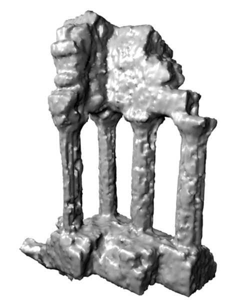
143 142 Chapter 5: The Gradient of the Reprojection Error Figure 5.10: First row: some of the input images of the temple dataset. Second row: surface evolution for the temple sparse ring dataset. Third row: final reconstruction for the temple sparse ring dataset. Forth row: final reconstruction for the dino sparse ring dataset.

144 5.8 Experiments 143 templering templesparsering accu. (mm) compl. (%) accu. (mm) compl. (%) Lambertian specular median worst best dinoring dinosparsering accu. (mm) compl. (%) accu. (mm) compl. (%) Lambertian specular median worst best Table 5.2: Results for the temple and dino datasets. For each dataset, accuracy and completeness scores are given for Lambertian model and for the model estimating a specular component. The median, the worst and the best scores submitted to the evaluation are given for comparison purposes. surface is trying to reconstruct the bench onto which the temple is standing. This is because we assume the background to be black, and the bench is dark, but not black. In the following section we present a simple extension of the model that palliates these two problems. In order to test the possibility of using the level set representation to reconstruct high-resolution models, we tested the algorithm on the Leuven dataset. The data set contains 7 high-resolution images (3000x2000 pixels) of a corner of the Leuven s City Hall. The resolution of the level set grid should be on a par with the resolution of the images, thus we downsampled the images. At the finest level of resolution, we used the images downsampled at 1500x1000 pixels and a voxel grid of 500x500x750 voxels. To avoid the memory cost of storing all these voxels, we used the Hierarchical Run Length Encoding sparse data structure [68] to store only the voxels in a narrowband arrown the surface. We also manually masked some parts of the images in order to reconstruct only the central part of the scene. Figure 5.11 shows the input images and the reconstructed model.

145 144 Chapter 5: The Gradient of the Reprojection Error Figure 5.11: The seven manually segmented input images of the Leuven s City Hall (top), and two renderings of the reconstructed surface.

146 5.8 Experiments Dealing with Non-Lambertian Effects Most real world scenes are not Lambertian. Even the temple and the dino objects, which were intentionally chosen for being Lambertian, exhibit a certain amount of specular reflection. In this section, we present a modification of the Lambertian model (5.54) to take into account deviations from the constant brightness assumption without explicitly modeling the reflectance properties of the scene. The idea is to consider that the predicted images are the sum of the images that would be produced by a Lambertian object, plus a specular component, and try to estimate both the Lambertian color C and the specular components of the images S : I R 3. In order to constrain the problem, we assume that the specular component will be smooth. Another issue with the previous model, is that the background was assumed to have a constant color. In the temple and dino images, this is clearly not the case. Ideally, we would have the images of the background without the object, but sometimes we don t. To solve this, we will also estimate the background images, F : I R 3, under the single assumption that these images are smooth. The predicted image is then I (u) = { (u)) + S(u) if π 1 Γ (u) Γ F(u) if π 1 Γ (u) B. (5.72) C(π 1 Γ The energy to be minimized for every image is E(Γ, C, S,F) = 1 ( I(u) I (u) ) 2 du 2 I + λ S 2 dx + λ F 2 du. 2 R 2 3 I (5.73) The minimization can be done by gradient descent on the surface Γ, the specular component S, and the background images B. The optimal Lambertian color C can still be computed directly as in the previous model, but removing the specular component from the input images first. The gradient of the energy with respect to the specular component, S, is ( I C S ) f λ S (5.74) where the foreground indicator function, f : I {0, 1}, is defined as f(u) = { 1 if π 1 Γ (u) Γ 0 if π 1 Γ (u) B. (5.75)

147 146 Chapter 5: The Gradient of the Reprojection Error Figure 5.12: Reconstruction obtained for the temple ring and dino ring datasets, while estimating the specular component and the background. The gradient with respect to the background image, F, is ( I F ) (1 f) λ F (5.76) We executed the minimization on the temple and dino datasets, to see whether the model improves the results. The accuracy and completeness scores appear in Table 5.2 under the label specular. All the scores improved very significantly with respect to the ones obtained without estimating the specular component (Lambertian label). Figure 5.12 shows the reconstructed models, where we can see, for example, that the stairs of the temple are better reconstructed, and that this time the bench is not recunstructed. Figure 5.13 we show some of the estimated specular and background images.

148 5.9 Conclusion 147 We observe that the estimated specular component, has a characteristic pattern in all the images: one side of the image is green while, the other is magenta. The green side always correspond to the upper part of the camera s sensor, and the magenta to the lower part. We think that this must be due to some chromatic aberration of the camera itself and not due to the reflectance properties of the objects. Thus, although the specular component estimation was added to deal with specularities, it turned out to be useful for correcting camera s errors. The estimated background images globally correspond to the real background. Near the silhouette of the objects a bit of foreground color is being estimated as background. This did apparently not affect the results. 5.9 Conclusion In this chapter we compute the derivative of the reprojection error functional. The difficult part has been to correctly take into account the visibility changes that occur while the surface moves, which is one of the most challenging problems in surface reconstruction from images. The reward is that it is now possible to minimize the reprojection error via surface evolution. The benefit of this minimization is that the reconstructed surface is the one that best reproduces the observed images. In particular, as demonstrated in the experiments, the evolution moves the contour generators of the surface so that the apparent contours appear at their correct location in the images. This is a direct consequence of the correct minimization of the reprojection error itself. Therefore, current methods using additional silhouettes or apparent contour constraints can now be understood and justified by the single criterion of the reprojection error.

149 148 Chapter 5: The Gradient of the Reprojection Error Figure 5.13: From left to right: the input image, the projection of the estimated Lambertian color, the estimated specular component, and the estimated background. The values of the specular and the background images are scaled for better visualization.