Rendering the Teapot 1

Transcription

1 Rendering the Teapot 1

2 Utah Teapot 2 Angel and Shreiner: Interactive Computer Graphics 7E Addison-Wesley 2015

3 vertices.js var numteapotvertices = 306; var vertices = [ vec3(1.4, 0.0, 2.4), vec3(1.4, , 2.4), vec3(0.784, -1.4, 2.4), vec3(0.0, -1.4, 2.4), vec3(1.3375, 0.0, ),... ]; 3

4 patches.js var numteapotpatches = 32; var indices = new Array(numTeapotPatches); indices[0] = [0, 1, 2, 3, 4, 5, 6, 7, 8, 9, 10, 11, 12, 13, 14, 15 ]; indices[1] = [3, 16, 17, 18,.. ]; 4

5 Evaluation of Polynomials 5

6 Modeling

7 Topics Introduce types of curves and surfaces Explicit Implicit Parametric Discuss Modeling and Approximations

8 Escaping Flatland Lines and flat polygons Fit well with graphics hardware Mathematically simple But world is not flat Need curves and curved surfaces At least at the application level Render them approximately with flat primitives

9 Modeling with Curves data points approximating curve interpolating data point 9

10 Good Representation? Properties Stable Smooth Easy to evaluate Must we interpolate or can we just come close to data? Do we need derivatives?

11 Explicit Representation Function y=f(x) Cannot represent all curves Vertical lines Circles Extension to 3D y=f(x), z=g(x) The form z = f(x,y) defines a surface y z x y x

12 Implicit Representation Two dimensional curve(s) g(x,y)=0 Much more robust All lines ax+by+c=0 Circles x 2 +y 2 -r 2 =0 Three dimensions g(x,y,z)=0 defines a surface Intersect two surface to get a curve

13 Algebraic Surface i j k x i y j z k = 0 Quadric surface 2 i+j+k At most 10 terms 13

14 Parametric Curves Separate equation for each spatial variable x=x(u) y=y(u) z=z(u) For u max u u min we trace out a curve in two or three dimensions p(u min ) p(u) p(u)=[x(u), y(u), z(u)] T p(u max ) 14

15 Parametric Lines We can normalize u to be over the interval (0,1) Line connecting two points p 0 and p 1 p(1)= p 1 p(u)=(1-u)p 0 +up 1 Ray from p 0 in the direction d p(u)=p 0 +ud p(0) = p 0 d p(0) = p 0 p(1)= p 0 +d 15

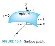
16 Parametric Surfaces Surfaces require 2 parameters x=x(u,v) y=y(u,v) z=z(u,v) p(u,v) = [x(u,v), y(u,v), z(u,v)] T Want same properties as curves: Smoothness Differentiability Ease of evaluation y p(u,1) p(0,v) x z p(u,0) p(1,v) 16

17 17 Normals We can differentiate with respect to u and v to obtain the normal at any point p = u v u u v u u v u u v u ) /, z( ) /, y( ) /, x( ), p( = v v u v v u v v u v v u ) /, z( ) /, y( ) /, x( ), p( v v u u v u = ), ( ), p( p n

18 Curve Segments p(u) join point p(1) = q(0) p(0) q(u) q(1) 18

19 Parametric Polynomial Curves N i j x( u) = cxi u y( u) = cyj u z( u) = czk u i= 0 M j= 0 If N=M=L, we need to determine 3(N+1) coefficients L k = 0 Curves for x, y and z are independent, we can define each independently in an identical manner k We will use the form where p can be any of x, y, z p( u) = L k = 0 c k u k 19

20 Why Polynomials Easy to evaluate Continuous and differentiable everywhere Continuity at join points including continuity of derivatives p(u) q(u) join point p(1) = q(0) but p (1) q (0)

21 Cubic Polynomials N=M=L=3, p( u) = 3 k = 0 c k u k Four coefficients to determine for each of x, y and z Seek four independent conditions for various values of u resulting in 4 equations in 4 unknowns for each of x, y and z Conditions are a mixture of continuity requirements at the join points and conditions for fitting the data

22 22 Matrix-Vector Form u c u k k k = = 3 0 ) p( = c c c c c = u u u u define u c c u T T u = = ) p( then

23 Interpolating Curve p 1 p 3 p 0 p 2 Given four data (control) points p 0, p 1,p 2, p 3 determine cubic p(u) which passes through them Must find c 0,c 1,c 2, c 3 23 p( u) = T 3 k = 0 c p( u ) = u c = k u c T k u

24 24 Interpolation Equations apply the interpolating conditions at u=0, 1/3, 2/3, 1 p 0 =p(0)=c 0 p 1 =p(1/3)=c 0 +(1/3)c 1 +(1/3) 2 c 2 +(1/3) 3 c 2 p 2 =p(2/3)=c 0 +(2/3)c 1 +(2/3) 2 c 2 +(2/3) 3 c 2 p 3 =p(1)=c 0 +c 1 +c 2 +c 2 or in matrix form with p = [p 0 p 1 p 2 p 3 ] T p=ac = A

25 Interpolation Matrix Solving for c we find the interpolation matrix MI = 1 A = c=m I p Note that M I does not depend on input data and can be used for each segment in x, y, and z 25

26 Interpolating Multiple Segments use p = [p 0 p 1 p 2 p 3 ] T use p = [p 3 p 4 p 5 p 6 ] T Get continuity at join points but not continuity of derivatives 26

27 Blending Functions Rewriting the equation for p(u) p(u)=u T c=u T M I p = b(u) T p where b(u) = [b 0 (u) b 1 (u) b 2 (u) b 3 (u)] T is an array of blending polynomials such that p(u) = b 0 (u)p 0 + b 1 (u)p 1 + b 2 (u)p 2 + b 3 (u)p 3 b 0 (u) = -4.5(u-1/3)(u-2/3)(u-1) b 1 (u) = 13.5u (u-2/3)(u-1) b 2 (u) = -13.5u (u-1/3)(u-1) b 3 (u) = 4.5u (u-1/3)(u-2/3) 27

28 Blending Functions NOT GOOD b 0 (u) = -4.5(u-1/3)(u-2/3)(u-1) b 1 (u) = 13.5u (u-2/3)(u-1) b 2 (u) = -13.5u (u-1/3)(u-1) b 3 (u) = 4.5u (u-1/3)(u-2/3) 28

29 As Opposed to

30 Parametric Surface

31 Cubic Polynomial Surfaces p(u,v)=[x(u,v), y(u,v), z(u,v)] T where p( u, v) = 3 3 ciju i= 0 j= 0 i v j p is any of x, y or z Need 48 coefficients ( 3 independent sets of 16) to determine a surface patch 31

32 Interpolating Patch p( u, v) = 3 i= o 3 j= 0 c ij u i v j Need 16 conditions to determine the 16 coefficients c ij Choose at u,v = 0, 1/3, 2/3, 1 32

33 Matrix Form Define v = [1 v v 2 v 3 ] T C = [c ij ] P = [p ij ] p(u,v) = u T Cv If we observe that for constant u (v), we obtain interpolating curve in v (u), we can show C=M I PM I p(u,v) = u T M I PM IT v 33

34 34 Blending Patches p v b u b v u p ij j j i o i ) ( ) ( ), ( = = = Each b i (u)b j (v) is a blending patch Shows that we can build and analyze surfaces from our knowledge of curves

35 Bezier and Spline Curves and Surfaces

36 Bezier

37 Bezier Surface Patches

38 Utah Teapot Bezier Avatar Available as a list of 306 3D vertices and the indices that define 32 Bezier patches 38

39 Bezier Do not usually have derivative data Bezier suggested using the same 4 data points as with the cubic interpolating curve to approximate the derivatives 39

40 Approximating Derivatives p 1 located at u=1/3 p 1 p 2 p 2 located at u=2/3 p p0 p'(0) 1/ 3 1 p p2 p'(1) 1/ 3 3 slope p (0) slope p (1) p 0 u p 3 40 Angel and Shreiner: Interactive Computer Graphics 7E Addison-Wesley 2015

41 Equations Interpolating conditions are the same p(0) = p 0 = c 0 p(1) = p 3 = c 0 +c 1 +c 2 +c 3 Approximating derivative conditions p (0) = 3(p 1 - p 0 ) = c 0 p (1) = 3(p 3 - p 2 ) = c 1 +2c 2 +3c 3 Solve four linear equations for c=m B p 41 Angel and Shreiner: Interactive Computer Graphics 7E Addison-Wesley 2015

42 42 Bezier Matrix = MB p(u) = u T M B p = b(u) T p blending functions

43 Blending Functions # 3 (1 u) & % 2( 3u(1 u) b(u) = % ( % 3u 2 (1 u) ( % ( $ ' 3 u Note that all zeros are at 0 and 1 which forces the functions to be smooth over (0,1) 43

44 Bernstein Polynomials b kd ( u) = d! k!( d u k)! k (1 u) d k Blending polynomials for any degree d All zeros at 0 and 1 For any degree they all sum to 1 They are all between 0 and 1 inside (0,1) 44

45 Rendering Curves and Surfaces 45

46 Evaluation of Polynomials 46

47 Evaluating Polynomials Polynomial curve evaluate polynomial at many points and form an approximating polyline Surfaces approximating mesh of triangles or quadrilaterals 47

48 Evaluate without Computation?

49 Convex Hull Property Bezier curves lie in the convex hull of their control points Do not interpolate all the data; cannot be too far away p 1 p 2 Bezier curve convex hull p 0 p 3 49

50 decasteljau Recursion Use convex hull property to obtain an efficient recursive method that does not require any function evaluations Uses only the values at the control points Based on the idea that any polynomial and any part of a polynomial is a Bezier polynomial for properly chosen control data 50

51 Splitting a Cubic Bezier p 0, p 1, p 2, p 3 determine a cubic Bezier polynomial and its convex hull Consider left half l(u) and right half r(u)

52 l(u) and r(u) Since l(u) and r(u) are Bezier curves, we should be able to find two sets of control points {l 0, l 1, l 2, l 3 } and {r 0, r 1, r 2, r 3 } that determine them

53 Convex Hulls {l 0, l 1, l 2, l 3 } and {r 0, r 1, r 2, r 3 }each have a convex hull that that is closer to p(u) than the convex hull of {p 0, p 1, p 2, p 3 } This is known as the variation diminishing property. The polyline from l 0 to l 3 (= r 0 ) to r 3 is an approximation to p(u). Repeating recursively we get better approximations.

54 Efficient Form l 0 = p 0 r 3 = p 3 l 1 = ½(p 0 + p 1 ) r 1 = ½(p 2 + p 3 ) l 2 = ½(l 1 + ½( p 1 + p 2 )) r 1 = ½(r 2 + ½( p 1 + p 2 )) l 3 = r 0 = ½(l 2 + r 1 ) Requires only shifts and adds! 54

55 Bezier in general Bezier Interpolating B Spline 55

56 Bezier Patches Using same data array P=[p ij ] as with interpolating form p( u, v) 3 3 = i= 0 j= 0 bi( u) b j ( v) p ij = u T M B PM T B v Patch lies in convex hull

57 Evaluation of Polynomials 57

58 decasteljau Recursion 58 Angel and Shreiner: Interactive Computer Graphics 7E Addison-Wesley 2015

59 Surfaces Recall that for a Bezier patch curves of constant u (or v) are Bezier curves in u (or v) First subdivide in u Process creates new points Some of the original points are discarded original and discarded original and kept new

60 Second Subdivision 16 final points for 1 of 4 patches created 60

61 Angel s Gifts Chapter 11, 7e vertices.js: three versions of the data vertex data patches.js: teapot patch data teapot1: wire frame teapot by recursive subdivision of Bezier curves teapot2: wire frame teapot using polynomial evaluation teapot3: same as teapot2 with rotation teapot4: shaded teapot using polynomial evaluation and exact normals teapot5: shaded teapot using polynomial evaluation and normals computed for each triangle

62 vertices.js var numteapotvertices = 306; var vertices = [ vec3(1.4, 0.0, 2.4), vec3(1.4, , 2.4), vec3(0.784, -1.4, 2.4), vec3(0.0, -1.4, 2.4), vec3(1.3375, 0.0, ),... ]; 62

63 patches.js var numteapotpatches = 32; var indices = new Array(numTeapotPatches); indices[0] = [0, 1, 2, 3, 4, 5, 6, 7, 8, 9, 10, 11, 12, 13, 14, 15 ]; indices[1] = [3, 16, 17, 18,.. ];

64 Patch Reader patchreader.js

65 Bezier Function Teapot 2 bezier = function(u) { var b = []; var a = 1-u; b.push(u*u*u); b.push(3*a*u*u); b.push(3*a*a*u); b.push(a*a*a); return b; } 65

66 Patch Indices to Data var h = 1.0/numDivisions; patch = new Array(numTeapotPatches); for(var i=0; i<numteapotpatches; i++) patch[i] = new Array(16); for(var i=0; i<numteapotpatches; i++) for(j=0; j<16; j++) { patch[i][j] = vec4([vertices[indices[i][j]][0], vertices[indices[i][j]][2], vertices[indices[i][j]][1], 1.0]); } 66

67 Vertex Data for ( var n = 0; n < numteapotpatches; n++ ) { var data = new Array(numDivisions+1); for(var j = 0; j<= numdivisions; j++) data[j] = new Array(numDivisions+1); for(var i=0; i<=numdivisions; i++) for(var j=0; j<= numdivisions; j++) { data[i][j] = vec4(0,0,0,1); var u = i*h; var v = j*h; var t = new Array(4); for(var ii=0; ii<4; ii++) t[ii]=new Array(4); for(var ii=0; ii<4; ii++) for(var jj=0; jj<4; jj++) t[ii][jj] = bezier(u)[ii]*bezier(v)[jj]; for(var ii=0; ii<4; ii++) for(var jj=0; jj<4; jj++) { temp = vec4(patch[n][4*ii+jj]); temp = scale( t[ii][jj], temp); data[i][j] = add(data[i][j], temp); } }

68 Quads for(var i=0; i<numdivisions; i++) for(var j =0; j<numdivisions; j++) { points.push(data[i][j]); points.push(data[i+1][j]); points.push(data[i+1][j+1]); points.push(data[i][j]); points.push(data[i+1][j+1]); points.push(data[i][j+1]); index += 6; } }

69 Recursive Subdivision 69 Angel and Shreiner: Interactive Computer Graphics 7E Addison-Wesley 2015

70 Divide Curve dividecurve = function( c, r, l){ // divides c into left (l) and right ( r ) curve data var mid = mix(c[1], c[2], 0.5); l[0] = vec4(c[0]); l[1] = mix(c[0], c[1], 0.5 ); l[2] = mix(l[1], mid, 0.5 ); r[3] = vec4(c[3]); r[2] = mix(c[2], c[3], 0.5 ); r[1] = mix( mid, r[2], 0.5 ); r[0] = mix(l[2], r[1], 0.5 ); l[3] = vec4(r[0]); return; }

71 Divide Patch dividepatch = function (p, count ) { if ( count > 0 ) { var a = mat4(); var b = mat4(); var t = mat4(); var q = mat4(); var r = mat4(); var s = mat4(); // subdivide curves in u direction, transpose results, divide // in u direction again (equivalent to subdivision in v) for ( var k = 0; k < 4; ++k ) { var pp = p[k]; var aa = vec4(); var bb = vec4(); 71

72 Divide Patch dividecurve( pp, aa, bb ); a[k] = vec4(aa); b[k] = vec4(bb); } a = transpose( a ); b = transpose( b ); for ( var k = 0; k < 4; ++k ) { var pp = vec4(a[k]); var aa = vec4(); var bb = vec4(); dividecurve( pp, aa, bb ); q[k] = vec4(aa); r[k] = vec4(bb); } for ( var k = 0; k < 4; ++k ) { var pp = vec4(b[k]); var aa = vec4(); 72

73 Divide Patch var bb = vec4(); dividecurve( pp, aa, bb ); t[k] = vec4(bb); } // recursive division of 4 resulting patches dividepatch( q, count - 1 ); dividepatch( r, count - 1 ); dividepatch( s, count - 1 ); dividepatch( t, count - 1 ); } else { drawpatch( p ); } return; } 73

74 Draw Patch drawpatch = function(p) { // Draw the quad (as two triangles) bounded by // corners of the Bezier patch points.push(p[0][0]); points.push(p[0][3]); points.push(p[3][3]); points.push(p[0][0]); points.push(p[3][3]); points.push(p[3][0]); index+=6; return; } 74 Angel and Shreiner: Interactive Computer Graphics 7E Addison-Wesley 2015

75 Vertex Shader <script id="vertex-shader" type="xshader/x-vertex"> attribute vec4 vposition; void main() { mat4 scale = mat4( 0.3, 0.0, 0.0, 0.0, 0.0, 0.3, 0.0, 0.0, 0.0, 0.0, 0.3, 0.0, 0.0, 0.0, 0.0, 1.0 ); gl_position = scale*vposition; } </script>

76 Fragment Shader <script id="fragment-shader" type="x-shader/x-fragment"> precision mediump float; void main() { gl_fragcolor = vec4(1.0, 0.0, 0.0, 1.0);; } </script>

77 Adding Shading WebGL/7E/11/teapot4.html Face Normals /teapot5.html 77 Angel and Shreiner: Interactive Computer Graphics 7E Addison-Wesley 2015

78 Using Face Normals var t1 = subtract(data[i+1][j], data[i][j]); var t2 =subtract(data[i+1][j+1], data[i][j]); var normal = cross(t1, t2); normal = normalize(normal); normal[3] = 0; points.push(data[i][j]); normals.push(normal); points.push(data[i+1][j]); normals.push(normal); points.push(data[i+1][j+1]); normals.push(normal); points.push(data[i][j]); normals.push(normal); points.push(data[i+1][j+1]); normals.push(normal); points.push(data[i][j+1]); normals.push(normal); index+= 6; 78

79 Exact Normals nbezier = function(u) { var b = []; b.push(3*u*u); b.push(3*u*(2-3*u)); b.push(3*(1-4*u+3*u*u)); b.push(-3*(1-u)*(1-u)); return b; }

80 Vertex Shader <script id="vertex-shader" type="x-shader/x-vertex > attribute vec4 vposition; attribute vec4 vnormal; varying vec4 fcolor; uniform vec4 ambientproduct, diffuseproduct, specularproduct; uniform mat4 modelviewmatrix; uniform mat4 projectionmatrix; uniform vec4 lightposition; uniform float shininess; uniform mat3 normalmatrix; void main() { vec3 pos = (modelviewmatrix * vposition).xyz; vec3 light = lightposition.xyz; vec3 L = normalize( light - pos ); vec3 E = normalize( -pos ); vec3 H = normalize( L + E ); // Transform vertex normal into eye coordinates vec3 N = normalize( normalmatrix*vnormal.xyz); // Compute terms in the illumination equation vec4 ambient = ambientproduct; float Kd = max( dot(l, N), 0.0 ); vec4 diffuse = Kd*diffuseProduct; float Ks = pow( max(dot(n, H), 0.0), shininess ); vec4 specular = Ks * specularproduct; if( dot(l, N) < 0.0 ) { specular = vec4(0.0, 0.0, 0.0, 1.0); } gl_position = projectionmatrix * modelviewmatrix * vposition; fcolor = ambient + diffuse +specular; fcolor.a = 1.0; } </script>

81 Fragment Shader <script id="fragment-shader" type="x-shader/xfragment"> precision mediump float; varying vec4 fcolor; void main() { gl_fragcolor = fcolor; } </script>

82 Post Geometry Shaders

83 Pipeline Polygon Soup

84 Pipeline

85 Topics Clipping Scan conversion

86 Clipping

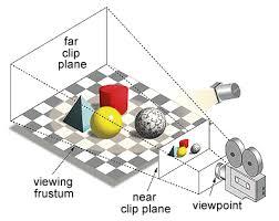
87 Clipping After geometric stage vertices assembled into primitives Must clip primitives that are outside view frustum

88 Clipping

89 Scan Conversion Which pixels can be affected by each primitive Fragment generation Rasterization or scan conversion

90 Additional Tasks Some tasks deferred until fragment processing Hidden surface removal Antialiasing

91 Clipping

92 Contexts 2D against clipping window 3D against clipping volume

93 2D Line Segments Brute force: compute intersections with all sides of clipping window Inefficient

94 Cohen-Sutherland Algorithm Eliminate cases without computing intersections Start with four lines of clipping window y = y max x = x min x = x max y = y min

95 The Cases Case 1: both endpoints of line segment inside all four lines Draw (accept) line segment as is y = y max x = x min x = x max y = y min Case 2: both endpoints outside all lines and on same side of a line Discard (reject) the line segment

96 The Cases Case 3: One endpoint inside, one outside Must do at least one intersection Case 4: Both outside May have part inside Must do at least one intersection y = y max x = x min x = x max

97 Defining Outcodes For each endpoint, define an outcode b 0 b 1 b 2 b 3 b 0 = 1 if y > y max, 0 otherwise b 1 = 1 if y < y min, 0 otherwise b 2 = 1 if x > x max, 0 otherwise b 3 = 1 if x < x min, 0 otherwise Outcodes divide space into 9 regions Computation of outcode requires at most 4 comparisons

98 Using Outcodes Consider the 5 cases below AB: outcode(a) = outcode(b) = 0 Accept line segment

99 Using Outcodes CD: outcode (C) = 0, outcode(d) 0 Compute intersection Location of 1 in outcode(d) marks edge to intersect with

100 Using Outcodes If there were a segment from A to a point in a region with 2 ones in outcode, we might have to do two intersections

101 Using Outcodes EF: outcode(e) logically ANDed with outcode(f) (bitwise) 0 Both outcodes have a 1 bit in the same place Line segment is outside clipping window reject

102 Using Outcodes GH and IJ same outcodes, neither zero but logical AND yields zero Shorten line by intersecting with sides of window Compute outcode of intersection new endpoint of shortened line segment Recurse algorithm

103 Cohen Sutherland in 3D Use 6-bit outcodes When needed, clip line segment against planes

104 Liang-Barsky Clipping Consider parametric form of a line segment p(α) = (1-α)p 1 + αp 2 1 α 0 p 1 p 2 Intersect with parallel slabs Pair for Y Pair for X Pair for Z

105 Liang-Barsky Clipping In (a): a 4 > a 3 > a 2 > a 1 Intersect right, top, left, bottom: shorten In (b): a 4 > a 2 > a 3 > a 1 Intersect right, left, top, bottom: reject

106 Advantages Can accept/reject as easily as with Cohen- Sutherland Using values of α, we do not have to use algorithm recursively as with C-S Extends to 3D

107 Polygon Clipping Not as simple as line segment clipping Clipping a line segment yields at most one line segment Clipping a polygon can yield multiple polygons Convex polygon is cool J 107

108 Fixes

109 Tessellation and Convexity Replace nonconvex (concave) polygons with triangular polygons (a tessellation) 109

110 Clipping as a Black Box Line segment clipping - takes in two vertices and produces either no vertices or vertices of a clipped segment 110

111 Pipeline Clipping - Line Segments Clipping side of window is independent of other sides Can use four independent clippers in a pipeline 111

112 Pipeline Clipping of Polygons Three dimensions: add front and back clippers Small increase in latency 112

113 Bounding Boxes Ue an axis-aligned bounding box or extent Smallest rectangle aligned with axes that encloses the polygon Simple to compute: max and min of x and y 113

114 Bounding boxes Can usually determine accept/reject based only on bounding box reject accept requires detailed clipping 114

115 Clipping vs. Visibility Clipping similar to hidden-surface removal Remove objects that are not visible to the camera Use visibility or occlusion testing early in the process to eliminate as many polygons as possible before going through the entire pipeline 115

116 Clipping

117 Hidden Surface Removal Object-space approach: use pairwise testing between polygons (objects) partially obscuring can draw independently Worst case complexity O(n 2 ) for n polygons 117

118 Better Still

119 Better Still

120 Painter s Algorithm Render polygons a back to front order so that polygons behind others are simply painted over B behind A as seen by viewer Fill B then A 120

121 Depth Sort Requires ordering of polygons first O(n log n) calculation for ordering Not all polygons front or behind all other polygons Order polygons and deal with easy cases first, harder later Polygons sorted by distance from COP 121

122 Easy Cases A lies behind all other polygons Can render Polygons overlap in z but not in either x or y Can render independently 122

123 Hard Cases Overlap in all directions but can one is fully on one side of the other cyclic overlap penetration 123

124 Back-Face Removal (Culling) face is visible iff 90 θ -90 equivalently cos θ 0 or v n 0 θ - plane of face has form ax + by +cz +d =0 - After normalization n = ( ) T + Need only test the sign of c - Will not work correctly if we have nonconvex objects 124

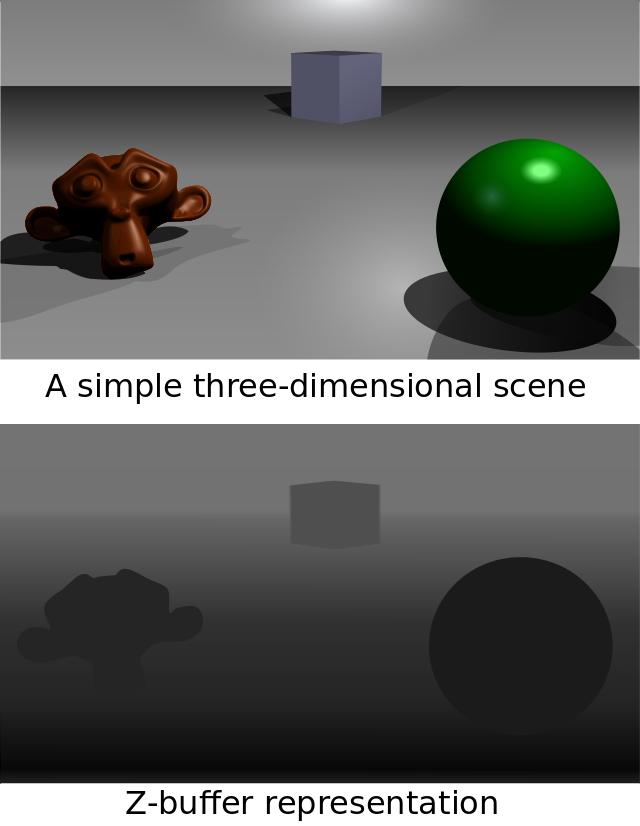
125 Image Space Approach Look at each ray (nm for an n x m frame buffer) Find closest of k polygons Complexity O(nmk) Ray tracing z-buffer 125

126 z-buffer Algorithm Use a buffer called z or depth buffer to store depth of closest object at each pixel found so far As we render each polygon, compare the depth of each pixel to depth in z buffer If less, place shade of pixel in color buffer and update z buffer 126

127 z-buffer for(each polygon P in the polygon list) do{ for(each pixel(x,y) that intersects P) do{ Calculate z-depth of P at (x,y) If (z-depth < z-buffer[x,y]) then{ z-buffer[x,y]=z-depth; COLOR(x,y)=Intensity of P at(x,y); } #If-programming-for alpha compositing: Else if (COLOR(x,y).opacity < 100%) then{ COLOR(x,y)=Superimpose COLOR(x,y) in front of Intensity of P at(x,y); } #Endif-programming-for } } display COLOR array.

128

129 Efficiency - Scanline As we move across a scan line, the depth changes satisfy aδx+bδy+cδz=0 Along scan line Δy = 0 Δz = - a c Δx In screen space Δx = 1 129

130 Scan-Line Algorithm Combine shading and hsr through scan line algorithm scan line i: no need for depth information, can only be in no or one polygon scan line j: need depth information only when in more than one polygon 130

131 Implementation Need a data structure to store Flag for each polygon (inside/outside) Incremental structure for scan lines that stores which edges are encountered Parameters for planes 131

132 Rasterization Rasterization (scan conversion) Determine which pixels that are inside primitive specified by a set of vertices Produces a set of fragments Fragments have a location (pixel location) and other attributes such color and texture coordinates that are determined by interpolating values at vertices Pixel colors determined later using color, texture, and other vertex properties

133 Scan-Line Rasterization

134 ScanConversion -Line Segments Start with line segment in window coordinates with integer values for endpoints Assume implementation has a write_pixel function Δy m = Δ x y = mx + h

135 DDA Algorithm Digital Differential Analyzer Line y=mx+ h satisfies differential equation dy/dx = m = Dy/Dx = y 2 -y 1 /x 2 -x 1 Along scan line Dx = 1 For(x=x1; x<=x2,ix++) { y+=m; display (x, round(y), line_color) }

136 Problem DDA = for each x plot pixel at closest y Problems for steep lines

137 Bresenham s Algorithm DDA requires one floating point addition per step Eliminate computations through Bresenham s algorithm Consider only 1 m 0 Other cases by symmetry Assume pixel centers are at half integers

138 Main Premise If we start at a pixel that has been written, there are only two candidates for the next pixel to be written into the frame buffer

139 Candidate Pixels 1 m 0 candidates last pixel Note that line could have passed through any part of this pixel

140 Decision Variable d = Δx(b-a) d is an integer d > 0 use upper pixel d < 0 use lower pixel -

141 Incremental Form Inspect d k at x = k d k+1 = d k 2Dy, if d k <0 d k+1 = d k 2(Dy- Dx), otherwise For each x, we need do only an integer addition and test Single instruction on graphics chips

142 Polygon Scan Conversion Scan Conversion = Fill How to tell inside from outside Convex easy Nonsimple difficult Odd even test Count edge crossings

143 Filling in the Frame Buffer Fill at end of pipeline Convex Polygons only Nonconvex polygons assumed to have been tessellated Shades (colors) have been computed for vertices (Gouraud shading) Combine with z-buffer algorithm March across scan lines interpolating shades Incremental work small

144 Using Interpolation C 1 C 2 C 3 specified by vertex shading C 4 determined by interpolating between C 1 and C 2 C 5 determined by interpolating between C 2 and C 3 interpolate between C 4 and C 5 along span C 1 scan line C 4 C 2 C 5 C 3 span

145 Scan Line Fill Can also fill by maintaining a data structure of all intersections of polygons with scan lines Sort by scan line Fill each span vertex order generated by vertex list desired order E. Angel and D. Shreiner: Interactive Computer Graphics 6E Addison-Wesley 2012

146 Data Structure

147 Aliasing Ideal rasterized line should be 1 pixel wide Choosing best y for each x (or visa versa) produces aliased raster lines E. Angel and D. Shreiner: Interactive Computer Graphics 6E Addison-Wesley 2012

148 Antialiasing by Area Averaging Color multiple pixels for each x depending on coverage by ideal line original antialiased magnified

149 Polygon Aliasing Aliasing problems can be serious for polygons Jaggedness of edges Small polygons neglected Need compositing so color of one polygon does not totally determine color of pixel All three polygons should contribute to color