Compression of Hyperspectral Images. A dissertation presented to. the faculty of. In partial fulfillment. of the requirements for the degree

Transcription

1 Compression of Hyperspectral Images A dissertation presented to the faculty of the Russ College of Engineering and Technology of Ohio University In partial fulfillment of the requirements for the degree Doctor of Philosophy Kai-Jen Cheng December Kai-Jen Cheng. All Rights Reserved.

2 2 This dissertation titled Compression of Hyperspectral Images by KAI-JEN CHENG has been approved for the School of Electrical Engineering and Computer Science and the Russ College of Engineering and Technology by Jeffrey C. Dill Professor of Electrical Engineering and Computer Science Dennis Irwin Dean, Russ College of Engineering and Technology

3 3 ABSTRACT CHENG, KAI-JEN, Ph.D., December 2013, Electrical Engineering Compression of Hyperspectral Images Director of Dissertation: Jeffrey C. Dill Hyperspectral images contain a wealth of spectral data, and occupy hundreds of megabytes, which makes the transmission to remote reception sites more challenging and difficult. Thus, compression schemes oriented to the task of remote transmission are becoming increasingly of interest in hyperspectral applications. In this dissertation, we develop a transform-based coding for high-dimensional hyperspectral images. We study Shapiro s EZW algorithm according to multiple modifications and the results show that the asymmetric transform and tree design have best performance in compression; in addition, the data dependent algorithm results in more compact outputs. We also present the performance of hybrid transforms, including the discrete wavelet transform and Karhunen-Loève transform, and the new asymmetric spatial-spectral tree structure. The results also show that the hybrid transform results in optimal energy distribution in spatial and spectral dimensions; moreover, the long spatial-spectral tree makes compression more efficient. We propose a Binary Embedded Zerotrees Wavelet (BEZW) algorithm for hyperspectral images. The zerotree quantization strategy of the BEZW is designed for the hybrid transformed images and the dual tree structures are defined in order to predict the insignificant pixels. For lossy hyperspectral image compression, the suitable quality criteria have to consider spectral information and reflect spectral loss. In this research we list spectral distortion measurements, examined distortion on lossy compression, and

4 4 compare their abilities to accurately characterize compression fidelity in end user applications, such as unsupervised classification of image pixels. Finally, we cover the lossy and lossless results of the BEZW algorithm on AVIRIS datasets and comparisons of the conventional transform-based coders and the best predictive coders in terms of the complexity and distortion criteria. The BEZW algorithm is competitive with the best predictive algorithms and also is an efficient computational method which is comparable to transform-based algorithms.

5 5 ACKNOWLEDGMENTS I would like to express my deepest appreciation to all those who provided me the possibility to complete this dissertation. I would like to offer my special thanks to my committee chair Professor Jeffrey Dill for his valuable and constructive suggestions during the planning and development of this research work without his guidance and persistent help this dissertation would not have been possible. I would also like to extend my thanks to my committee members, Professor Chris Bartone, Professor Bryan Riley, Professor Jundong Liu, Professor Sergio Lopez- Permouth, and Professor Martin J. Mohlenkamp for serving in this committee and providing me good suggestions on this dissertation work. Finally, I wish to thank Ya-ting Shih for her love, kindness and support during these years. Furthermore, I would like express my sincerely thanks to my parents, and my sisters for their support and encouragement.

6 6 TABLE OF CONTENTS Page Abstract...3 Acknowledgments...5 List of Tables...8 List of Figures Chapter 1 : Introduction The Scope of Remote Sensing Hyperspectral Imagery AVIRIS, CCSDS, and Hyperion Hyperspectral Imagery Compression Tradeoff Dissertation Objectives Dissertation Contribution Chapter 2 : Literature Review Predictive Coding Transform-Based Coding Vector Quantization Chapter 3 : One-Dimensional Mathematical Transforms Fourier Transform Discrete Cosine Transform (DCT) Wavelet Transform (WT) Continuous Wavelet Transform (CWT) Discrete Wavelet Transform (DWT) Lifting Scheme Karhunen-Loève Transform (KLT) Integer KLT Chapter 4 : Conventional Transform-Based Coding Zerotree-Based Coding Embedded Zerotree Wavelet (EZW) Set Partitioning In Hierarchical Trees (SPIHT)... 83

7 7 4.2 Zeroblocks-Based Coding Set Partitioned Embedded block (SPECK) Embedded ZeroBlock Coder (EZBC) Chapter 5 : Quality Criteria for Lossy Image Compression Chapter 6 : Compression Algorithm for Hyperspectral Images Symmetric Transform Asymmetric Transform Simulations and Performance Hybrid Transforms Binary EZW Algorithm (BEZW) Asymmetric Tree Structures Coding Sign Bits Separately Coding Magnitudes Lossless Compression Performance Lossy Compression Performance Chapter 7 : Conclusions and Future Work References

8 8 LIST OF TABLES Page Table 1 Research and Commercial imaging spectrometers [6] Table 2 Standard AVIRIS dataset [4] Table 3 CCSDS dataset [7] Table 4 Hyperion dataset [7] Table 5 Computational complexity of KLT and IKLT [55] Table 6 Pseudo-code of the EZW algorithm [36] Table 7 Pseudo-code of the SPIHT algorithm [42] Table 8 Pseudo-code of the SPECK algorithm [52] Table 9 Pseudo-code of the EZBC algorithm [51] Table 10 Main properties of wavelet families Table 11 Lossless compression results (bpppbs) of the EZW algorithm using various wavelet filters Table 12 Observing lossless compression results (bpppbs) of the EZW algorithm using bior2.4 under different levels of decomposition Table 13 Lossy compression results (PSNR in db) of the EZW algorithm using various wavelet filters Table 14 Lossless compression results (bpppbs) of the EZW algorithm under the wavelet packet transform Table 15 Lossless compression results (bpppbs) of the EZW algorithm under the adaptive wavelet packet transform

9 9 Table 16 Lossless compression results (bpppbs) of the EZW algorithm using Christophe asymmetric tree based on the wavelet packet transform Table 17 Examples of coded symbols generated by EZW algorithm for tree (b) and (d) Table 18 Numbers of coded symbols from the EZW algorithm with PZR/NZT and without PZR/NZT, using the bior-2.4 filter on Jasper Table 19 Numbers of coded symbols from the EZW algorithm with PZR/NZT and without PZR/NZT, using the bior-2.4 filter on Moffett Table 20 Lossless compression results (bpppbs) of the EZW algorithm with PZR/NZT Table 21 Lossless compression results (bpppbs) of the EZW algorithm using hybrid transform Table 22 Lossless compression results (bpppbs) of the EZW algorithm using Dragotti s asymmetric trees based on the hybrid transform Table 23 Lossless compression results (bpppbs) of the EZW algorithm using new 3D asymmetric trees based on hybrid transform Table 24 Lossless compression results for EZW algorithm with PZT/NZT using new 3D asymmetric trees based on the hybrid transform Table 25 A study of the bit rates generated by the EZW algorithm using new 3D asymmetric trees and the hybrid transform Table 26 Lossless compression results (bpppbs) of the residual EZW algorithm using new 3D asymmetric trees and hybrid transform

10 10 Table 27 Lossless compression results (bpppbs) of the residual EZW algorithm with PZT/NZT using new 3D asymmetric trees and hybrid transform Table 28 Sign bit distribution of the transformed image (Moffett01 with size 512x512x224) over a range of lossy threshold values Table 29 Results of two sign coding methods, arithmetic coding (AC) and EZW, in bit per pixel per band (bpppb), encoding Moffett01 (512x512x224) Table 30 The pseudocode for the BEZW algorithm Table 31 Lossless compression results (bpppbs) of the BEZW algorithm using new 3D asymmetric trees and hybrid transform Table 32 Comparison of bpppbs for transform-based algorithms on AVIRIS images Table 33 Lossless Compression results in bpppbs for 16 bits calibrated AVIRIS images Table 34 Lossless compression results in bpppbs for 16 bits uncalibrated CCSDS images Table 35 Compression results in bpppbs for 16 bits calibrated CCSDS AVIRIS images Table 36 Lossless compression results in bpppbs for 12 bits raw CCSDS AVIRIS images Table 37 Lossless compression results in bpppbs for 12 bits Hyperion Hyperspectral Images

11 11 Table 38 Quality criteria of MSS, MSA, MSID and AC (%) on AVIRIS hyperspectral images. On MSS, MSA and MSID less is better Table 39 Quality criteria of MSS, MSA, MSID and AC (%) on CCSDS hyperspectral images

12 12 LIST OF FIGURES Page Figure 1. Perspective of AVIRIS hyperspectral image cube of spatial data(x and y) and spectral data (z) [4]. Each continuous spectral trace for each image pixel is unique Figure 2. Classic AVIRIS dataset used for compression algorithm evaluation [4] Figure 3. False-color CCSDS dataset used for compression algorithm evaluation [7] Figure 4. False-color Hyperion dataset used for compression algorithm evaluation [7].. 28 Figure 5. Examples of mother wavelets [77] Figure 6. Two-channel analysis and synthesis filter bank [38] Figure 7. Three-level dyadic wavelet decomposition [38] Figure 8. Subbands and energy distribution after 2-level DWT decomposition Figure 9. Diagram of the forward wavelet transform by use of lifting [87] Figure level DWT wavelet decomposition using the lifting scheme [87] Figure 11. Formation of a vector from corresponding pixels in a hyperspectral image Figure 12. Distributions of energy (db) of each original image band and KLT band for Moffett01 and Jasper Figure 13. Lifting scheme of the forward IKLT for 4-Band image [90] Figure 14. Lifting scheme of the backward IKLT for 4-Band image [90] Figure 15. Bitplane representation Figure 16. Raster and Morton Scan Orders [38] Figure 17. Illustration of wavelet decomposition and 2D quad-tree structure... 79

13 13 Figure 18. Illustration of wavelet decomposition and SPIHT tree structure. denotes offspring set. denotes grand-descendant set. denotes full descendant set Figure 19. Partitioning of image into set S 0 and I [52] Figure 20. Partitioning of set S 0 [52] Figure 21. Partitioning of set I [52] Figure 22. Illustration of quad-tree [51] Figure 23. (a) Classical two-level 3D dyadic wavelet decomposition and (b) symmetric 3D quad-tree Figure 24. Subbands of a 2-level wavelet packet transform and Christophe s asymmetric 3D tree structure [9] Figure 25. Line wavelet transform in the spectral dimensions [38] Figure 26. (a) Uniform wavelet transform. (b) Adaptive wavelet packet transform [38] Figure 27 The spatial shift of Bior 4.4, Db6 and Sym Figure 28. Explanation of (a) ZRT (b) POS/NEG (c) IZ and (d) PZT/NZT Figure 29. Each IKLT band is decomposed to 7 subbands with 2D-IDWT for 2 levels. 120 Figure 30. Asymmetric tree structure Figure 31. Subband parent-children relationships for 224 bands after a two-level 2D- IDWT Figure 32. System diagram Figure 33. Percentages of energy in Ea1, Eh1, Ed1, and Ev1 on each transformed IKLT band for (a) Moffett01, (b) Jasper01, and (c) LowAltitude01 with 1 level 2D-IDWT

14 14 Figure 34. Perspective of asymmetrical dual-tree (a) Upper Tree: Parent-children relationships for top M bands after a two-level 2D-IDWT and (b) Lower Tree: Parentchildren relations between Band M+1 and the last band Figure 35. The rate-distortion performance of 3D-BEZW on comparison with the different transform-based methods [53] carrying on standard AVIRIS images Figure 36. Quality evaluations of 3D-BEZW and 3DSPIHT on Moffett scene01 in terms of MSA, MSS, and MSID

15 15 CHAPTER 1 : INTRODUCTION 1.1 The Scope of Remote Sensing Remote sensing is the science of deriving information about the earth s surface from a great distance using optical sensors without physical contact with the object. The evolution of the science is strongly related to the practice of photography [1]. In 1858, the first aerial photos were taken by Gaspard-Félix Tournachon from a tethered balloon over Paris, France. Other pioneer photographers also used rockets, kites and pigeons to carry their cameras. In the early stage of aerial photography, managing the cameras on these carriers was very difficult and unreliable. In the early 1900s, the airplane was invented. In 1909, Wilbur Wright took the first aerial photos from an airplane under controlled speed, altitude, and direction. During World War I, the role of aerial photography became more important. Many applications of aerial photography were used in military reconnaissance and surveillance. Specially designed cameras and relevant aerial instruments for aircrafts were developed and devised by the U.S. government. Following the end of war, some pioneering civilian companies converted these military applications of aerial photography into non-military applications such as geologic mapping or a series of soil, forest, and agricultural surveys. In World War II, the significance of aerial intelligence was increased greatly, because the expansion of aerial reconnaissance reached deeper within enemy territory to capture valuable information such as military deployment, as well as industrial and transportation infrastructures. After the war, many experienced pilots, camera operators, and photo-interpreters, who were trained by the government or the military, applied their

16 16 valuable skills and experiences to civilian companies, and where they flourished in the remote sensing industry. In the 1960s, there were significant changes and improvements in the history of remote sensing. The first successful and dedicated low Earth orbital weather satellite (Television Infrared Observation Satellite, or TIROS-1) was launched by NASA on April 1, 1960 [2]. It was first designed for climatological and meteorological observation of Earth and provided the basis for the later development of land observation satellites. TIROS-1 carried infrared radiometers observing Earth's heat distribution and brought the aerial photography into the infrared and microwave regions. Since new forms of images were collected using radiation outside the visible region of the spectrum, the term, aerial photography, was no longer suitable to describe the new form of imagery. The new term, remote sensing, emerged and began to be used in At that time, many classified remote sensing techniques and instruments released by the military accelerated the growth of remote sensing in scientific and civilian applications. The Earth-orbiting satellite, Landsat 1, originally named "Earth Resources Technology Satellite 1", was launched on July 23, 1972 [3]. Landsat program was initiated for the study of the Earth s surface and resources. Its space-based sensor, called a multispectral scanner (MSS), allowed it to acquire four-band multispectral imagery on agricultural and forestry resources, geology and mineral resources, hydrology and water resources, geography and marine resources, and meteorological phenomena. Besides its space-based sensor, the Landsat 1 s most important contribution was providing the standard digital format of multispectral images. That digital format facilitated in precise

17 17 processing, acquisition, reproduction, and distribution of remotely sensed images; moreover, this standard digital format encouraged the growth of the digital image processing field. Landsat 1 paved the way for the other satellites in the Landsat program, which is longest-running space program until the present. Two new MSS systems, Thematic Mapper (TM) and Enhanced Thematic Plus (ETM+) were installed on later Landsat series. The commercial Earth observation satellite, IKONOS, was first operated for civilian applications and had available high-spatial resolution of multispectral and panchromatic imagery at 1-m and 4-m resolutions [1]. The IKONOS imagery is suitable for applications requiring a high level of detail and accuracy, such as mapping, and urban planning. In the 1980s, the Jet Propulsion Laboratory (JPL), developed the hyperspectral spectrometer, began the era of hyperspectral remote sensing [4]. The advanced Airborne Visible/Infrared Imaging Spectrometer (AVIRIS) has been flown on four aircraft platforms: NASA's ER-2 jet, Twin Otter International's turboprop, Scaled Composites' Proteus, and NASA's WB-57.The spectrometer produces up to 224 spectral bands about 10nm wide, over the spectrum from 400 to 2500 nanometers (nm). With such high spectral resolution, many subtle objects and materials can be identified. It has been used in terrain classification, environmental monitoring, agricultural monitoring, geological exploration and surveillance.

18 18 HYperspectral Digital Imagery Collection Experiment (HYDICE) was one of the airborne hyperspectral instruments used at relatively low altitudes. It was operated in 1994 and produces 210 spectral bands between 400 and 2500 nm [1]. Hyperion was on NASA s Earth-Observing 1 (EO 1) satellite as the first civilian hyperspectral satellite system operated in It has provided images in 220 spectral bands over the range 400 to 2500 nm [2]. Global remote sensing acquires and monitors the broad-scale observation of the land surface and surrounding coastal regions for global change research, regional environmental change studies and other civil and commercial purposes. On December 1999, NASA launched Terra-1, the first satellite of a system specifically designed to acquire global coverage to provide the foundations for documenting environmental changes during recent decades [5]. The Terra-1 satellite carries five modern instruments that take coincident measurements of the Earth s system: Advanced Spaceborne Thermal Emission and Reflection Radiometer (ASTER), Clouds and Earth's Radiant Energy System (CERES), Measurements Of Pollution In The Troposphere (MOPITT), MODerate-resolution Imaging Spectroradiometer (MODIS), and Multi-angle Imaging SpectroRadiometer (MISR). In contemporary remote sensors, improvements have focused on sensor size, swath width, signal-to-noise ratio, radiometric and spectral calibration accuracy, and spectral channels. Some examples of airborne and spaceborne sensors [6] are shown below in Table 1.

19 19 Table 1 Research and Commercial imaging spectrometers [6] AIRBORNE SENSOR Explanation of Acronym NUMBER OF BANDS WAVELENGTH RANGE ( ) AVIRIS Airborne Visible/InfraRed Imaging Spectrometer AHI Airborne Hyperspectral Imager ARCHER Airborne Real-time Cueing Hyperspectral Enhanced Reconnaissance AISA Airborne Imaging Spectrometer for Application CASI Compact Airborne Spectrographic Imager COMPASS COMPact Airborne Spectral Sensor HYDICE HYperspectral Digital Imagery Collection Experiment HyMap SPACEBORNE NUMBER WAVELENGTH STAND FOR SENSOR OF BANDS RANGE ( ) Hyperion FTHSI Fourier Transform Hyperspectral Imager Hyperspectral Imagery Three available hyperspectral datasets are represented and discussed in this section. In general, a hyperspectral spectrometer analyzes and interprets the measurement of electromagnetic radiations that are reflected from or emitted by targets on Earth s land, ocean or desert to produce hyperspectral images. Basically, a spectrometer mounted on an aircraft or satellite disperses the light into hundreds of narrow and adjacent spectra. Meanwhile, hundreds of sensors inside the spectrometer detector have individually corresponding spectrum, and they plot a digital hyperspectral image cube with hundreds

20 20 of contiguous spectral bands, as depicted in Figure 1. Each image cube is comprised of a three-dimensional array of pixels. A pixel is described by the intensity value and location in the three-dimensional image. The intensity value of a pixel represents the average value of a measured physical signal such as the solar radiance, emitted infrared radiation, or backscattered radar intensity reflected from the whole ground area. The intensity of a pixel is digitized and recorded as a digital number AVIRIS, CCSDS, and Hyperion Airborne Visible/InfraRed Imaging Spectrometer (AVIRIS) was acquired by the NASA Jet Propulsion Laboratory (JPL) in AVIRIS images provide more accurate and detailed information than other types of spectral data because of AVIRIS s abundant spectral information. AVIRIS was carried on a NASA ER-2 airplane over an altitude of approximately 20 km at about 730 km/hr. AVIRIS was the first image spectrometer to analyze the solar reflected radiance in 224 contiguous spectral bands with wavelengths from 400 to 2500nm. In an AVIRS image, each pixel resolution is called a scene corresponding to an area of approximately 11 km 10 km on the ground. Onboard storage saves all collected scenes along with navigation and engineering data and the readings from the AVIRIS onboard calibrator. When all data are processed and stored on the ground, each scene yields approximately 140 Megabytes (MB). An AVIRIS hyperspectral image can be regarded as a three-dimensional (3D) image cube with spatial dimensions formed by x and y axes and the spectral dimension (z). Figure 1 shows an AVIRIS image cube covering an area over Moffett Field, California, at the southern end of the San Francisco Bay. The cube displays a stack of 224 contiguous spectral bands

21 21 from the top of the visible region (400 nm) to the bottom of the infrared (2500 nm). The sides are in pseudo-color, ranging from black and blue (low frequency) to red (high frequency). Continuous spectral traces are also shown in Figure 1 and formed by observing a pixel column along the z direction. Three unique spectral traces represent urban, water and land, and it is possible to identify or distinguish different materials by comparing the spectral trace with the given spectral database Pixel Spectrum 2500 Pixel Spectrum radiance radiance Number of Band Number of Band 3500 Pixel Spectrum Spectral (z) radiance Spatial (y) Spatial (x) Number of Band Figure 1. Perspective of AVIRIS hyperspectral image cube of spatial data(x and y) and spectral data (z) [4]. Each continuous spectral trace for each image pixel is unique.

22 22 Table 2 lists the features of the five available calibrated AVIRIS images, Moffett Field, Jasper Ridge, Cuprite, Lunar Lake and Low Altitude. This is a standard dataset and is widely used in other published articles and methods. These data are made available on JPL s webpage [4]. The entire image contains 614 samples, 224 bands and lines are indicated in Table 2 and are stored as 16-bit signed integers. Each image is divided into multiple scenes with 512 lines and the last scene may be less than 512. To calculate the number of lines the file size must be divided by 275,072 bytes per line. The raw data size of a hyperspectral image is very large. Image compression is the best and most necessary solution to alleviate the pressure from the transmission, processing, and archiving of these large datasets. A Quick-look at these images is presented in Figure 2. Moffett Field and Jasper Ridge are a mix of urban area, water, and vegetation. Cuprite and Lunar Lake are more geologic features. Low Altitude represents a high spatial correlative structure in an urban area. Table 2 Standard AVIRIS dataset [4] Image Names Size (samples x/lines y/bands z) Features Moffett Field 614x2031x224 Vegetation, urban, water Jasper Ridge 614x2586x224 Vegetation Cuprite 614x2206x224 Geological features Lunar Lake 614x1431x224 Calibration Low Altitude 614x1087x224 High spatial resolution This newer set of AVIRIS images, which contains both calibrated and raw (uncalibrated) images, is made available for compression experiments and testing in

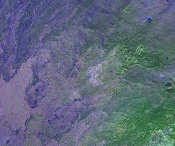
23 23 Table 3 and it is available on the JPL [7]. The dataset, provided by the Consultative Committee for Space Data System (CCSDS), has calibrated and raw 16-bit images from Yellowstone, Wyoming and two raw 12-bit images from Hawaii and Maine. Each image is a 512-line scene with 224 spectral bands and samples are indicated in Table 3. The quick-look also can be seen in Figure 3. Table 3 CCSDS dataset [7] Image Size Bit Scene number Names (samples/lines/bands) depth Type Yellowstone 677x512x224 0,3,10,11,18 16 Calibrated Yellowstone 680x512x224 0,3,10,11,18 16 Uncalibrated Hawaii 614 x512x Uncalibrated Maine 680 x512x Uncalibrated These Hyperion raw images are provided by the EO-1 Mission, NASA/USGS, and are also available on the JPL website [7] in Table 4. Each image has a width of 256 samples and, 242 spectral channels, and the lines are indicated in the below table. The Hyperion imager produces 12-bit data. Each pixel is stored as a 2-byte unsigned integer in Band Interleaved by Pixel (BIP) order. The false-color browse images are in Figure 4. Table 4 Hyperion dataset [7] Image Names Size (samples/lines/bands) Scene number Bit depth Type Lake Monona 256x3176x Vegetation, urban, water Mt. St. Helens 256x3242x Vegetation Erta Ale 256x3187x Vegetation, urban, water

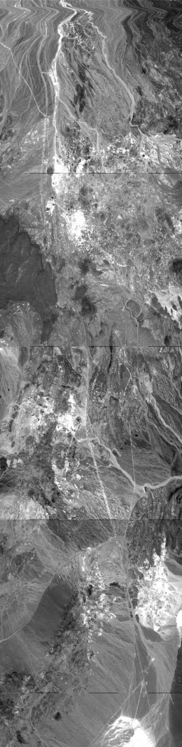
24 Moffett Jasper Ridge Cuprite 24

25 25 Lunar Lake Low Altitude Figure 2. Classic AVIRIS dataset used for compression algorithm evaluation [4].

26 26 1. Yellowstone Scene 0 (calibrated). 2. Yellowstone Scene 3 (calibrated) 3. Yellowstone Scene 10 (calibrated) 4 Yellowstone Scene 11 (calibrated) 5. Yellowstone Scene 18 (calibrated) 6 Hawaii Scene 1 (uncalibrated)

27 27 7. Maine Scene 10 (uncalibrated) Figure 3. False-color CCSDS dataset used for compression algorithm evaluation [7].

28 28 Mt. St. Helens Lake Monona Erta Ale Figure 4. False-color Hyperion dataset used for compression algorithm evaluation [7].

29 Hyperspectral Imagery Compression Tradeoff The benefits of compressing hyperspectral images [8] are: a) the reduction of transmission channel bandwidth; b) the reduction of the buffering and storage requirement; c) the reduction of data transmission time at a given rate. Because of the limited available resources and processing capabilities in spaceborne and airborne platforms, onboard encoding complexity is an important issue in hyperspectral compressions. Compression considers the tradeoff among these factors: processing capabilities, end-user applications and data quality (lossless or lossy), and constraints (memory and hardware) of spaceborne and airborne instruments. The greatest challenges are addressed on onboard image compression. First at all, due to the large amount of data collected and the limited transmission capacity, there is no doubt that the data have to be stored on the satellite or aircraft. However, this onboard storage is limited. The data have to be processed on the fly as they are acquired. The image compression algorithm has to be executed on the fly, that is, they have to start being compressed as images are acquired. Moreover, the compression has to be a low-complexity algorithm and have constant throughput because of the limited processing capability. Image compression is a technique for removing redundancy. Inherently image compression techniques are categorized into two groups: lossless and lossy compression. Lossless compression has no impact on the original image. The most recent publications show that the lossless compression ratio can be up to 4:1. However, it may not be sufficient to meet the constraint for onboard applications. On the contrary, lossy compression introduces small distortions in the original image and can reach much higher

30 30 compression ratio while discarding more information. The compromise of lossy compression is the ability to collect more images on the limited onboard storage. The effects of distortion on collected images differ from one case to another. The analysis and understanding of the distortion could be indicated by either subjective or objective image quality evaluation. Subjective evaluation uses human subjects to evaluate, compare or assess the quality of images. Objective evaluation assesses qualities by taking statistical measurements on test images. Other important properties of hyperspectral image compression include random access, progressive decoding, resolution scalability, standard format, and flexibility. The property of random access is to encode and decode selected portions of interest in a hyperspectral image. Since a small portion is encoded instead of the entire image, it reaches a high compression ratio without sacrificing any information in the image and can be reconstructed at high quality. The feature of progressive decoding is that the reconstruction fidelity is improved as more information is regained. Resolution scalability enables the generation of a low-resolution or coarse image for a quick preview of the entire image. If necessary, the low resolution image can be improved (less distortion) when more data are recovered. 1.4 Dissertation Objectives The current trend of airborne sensors is towards an increase in spatial resolution, spectral channels, and radiometric calibration accuracy, leading to a larger image size. It will greatly increase the computer processing requirements for image analysis and processing. In addition, since hyperspectral images are collected on remote acquisition

31 31 platforms such as satellites and aircrafts, the transmission of such data to remote reception sites can be a critical issue. Thus, compression schemes oriented to the task of remote transmission are becoming increasingly of interest in hyperspectral applications. A number of approaches have been proposed for compressing hyperspectral images in recently years. These approaches can be grouped into predictive coding, vector quantization and transform-based coding. The most popular method is predictive coding because of its superior lossless performance. Predictive coding requires complicated calculations and relies on sided information to implement the sophisticated predictors that produce the optimal differences between predicted and actual values. However, the high complexity of the optimal coding method might not be feasible onboard. On the contrary, the transform-based coding compresses a transformed image without requiring any prior information and complicated mathematics. In addition, transform-based coding is more efficient and simpler because of the useful properties of energy compaction and decorrelated data in the transformed image. Overall, transform-based coding is a good candidate for onboard hyperspectral data. Now, the leading transform-based coding algorithm (called the Set Partitioning In Hierarchical Trees, or SPIHT) is currently flying towards the 67P/Churyumov-Gerasimenko comet and is targeted to reach it in 2014 (Rosetta mission). This modified version of SPIHT is used to compress the hyperspectral data of the Visible and Infrared Thermal Imaging Spectrometer (VIRTIS) instrument [9]. A majority of the papers on transform-based coding recommend the use of symmetric 3D wavelet transform for hyperspectral images. However, some papers [10-13] have discussed that an asymmetric wavelet transform is more suitable for hyperspectral

32 32 images. Among these asymmetric transforms, few papers discuss the performance of the hybrid asymmetric transforms that combine the wavelet transform and principal component analysis (PCA). In this dissertation, implementation of the hybrid transform will be investigated in order to provide the optimal energy distribution and to study its performance. Our proposed image compression is inspired by Shapiro s Embedded Zerotrees Wavelet (EZW) algorithm. The proposed algorithm compresses the image by taking advantage of novel tree structures. In order to compress the new structure of the transformed images, the image compression needs to solve the following questions: 1) Can the tree structure strategy be applied to the hybrid transformed images? 2) If so, how can the tree structure be defined in order to predict the insignificant pixels? These questions will be examined in this dissertation. Image compression can be lossless and lossy; however, there is no universal quality evaluation or distortion measure that corresponds well to the impact of degradation on end user applications. The common criteria found in other papers are: signal to noise ratio (SNR), peak SNR and mean square error (MSE). However, for hyperspectral images, the suitable quality criteria have to consider spectral information, and reflect spectral loss. In this research we will examine a number of proposed measures of distortion, and compare their ability to accurately characterize compression fidelity in end-user applications, such as the unsupervised classification of image pixels.

33 Dissertation Contribution During the period of this dissertation work, the following papers have been published. 1. K. Cheng and J. Dill, "Hyperspectral images lossless compression using the 3D binary EZW algorithm," Image Processing: Algorithms and Systems XI, SPIE conference, pp , February 19, K. Cheng and J. Dill, "Lossless to lossy compression for hyperspectral imagery based on wavelet and 3D binary EZW," Defense, Security, and Sensing, SPIE conference, Baltimore, MD, April 29, K. Cheng and J. Dill, Efficient Lossless Compression for Hyperspectral Data Based on Integer Wavelets and 3D Binary EZW Algorithm," ASPRS Conference, Baltimore, MD, March 24, K. Cheng and J. Dill, An Improved EZW Hyperspectral Image Compression, 2nd International Conference on Signal and Image Processing (CSIP 2014), Shenzhen, China, January 12, K. Cheng and J. Dill, Lossless to Lossy Dual-Tree BEZW Compression for Hyperspectral Images", in IEEE Transactions on Geoscience and remote sensing

34 34 CHAPTER 2 : LITERATURE REVIEW A great variety of compression techniques have been proposed in the past few years while researchers consider the possible relations between larger volume of spatial and spectral information. In general, these image compression techniques are categorized into three groups: predictive coding, vector quantization, and transform-based coding. The following sections introduce the literature relevant to the compressions of hyperspectral images. 2.1 Predictive Coding The preferred method for lossless compressions of hyperspectral images is predictive coding. In its first step, single or multiple predictors are computed and used to create the residual errors and remove redundancy in the image. These errors are then encoded by entropy coding (Huffman coding, Rice coding, or arithmetic coding). Previous works have shown that the algorithm exploring the spectral correlation in hyperspectral images can compute the optimal predictors to reduce more redundancy in an image and results in high compression ratios. Note that in this discussion, all compression ratios are fundamentally data dependent, and will vary somewhat from image to image for the same compression algorithm. Roger and Cavenor [14] first studied Adaptive Differential Pulse-Code Modulation (ADPCM) for the lossless compression of AVIRIS hyperspectral images in They experimented on hyperspectral images with five sets of linear spatial, spectral and spatial-spectral predictors. Residual values are encoded by a Variable-Length Coding (VLC) algorithm. The compression ratio is stated in terms of bits per pixel per band

35 35 (bpppb), that is, the number of output bit stream is averaged over the entire image volume. Their lossless compression ratios for AVIRIS images are in the range :1. Rizzo et al. [15] proposed the lossless compression of hyperspectral image via Linear Prediction (LP). The simple spectral LP predicts the current pixel by its causal neighbor data set in the current band and previous band. Rizzo et al. s second method was called Spectral Least-SQuare (SLSQ) predictor, the optimal coefficients of which are determined by the Least Square (LS) algorithm. The algorithm exploring spectral correlations of hyperspectral image achieves better performance. Each pixel in each band was predicted by its own optimal SLSQ predictors such that the compression ratio was improved in the higher range 2-3:1, but the memory requirement was larger. Several researchers, who will be discussed in the following paragraphs, attempted to find optimized coefficients for predictors based on a group of pixels with similar properties. Aiazzi et al. contributed research focused on the optimized coefficient predictors by classification techniques [16-18]. In [16] a spatial and spectral Fuzzy DPCM is introduced. The 3D neighborhood (jointly spatial and spectral) for each pixel is defined and grouped into M clusters by Fuzzy C Means (FCM) [19]. Coefficients of predictor for each cluster are computed by the LS algorithm. The final estimate is computed as the weighted sum of all the outputs of predictors, where the weights are the similarity degrees. The prediction residuals are then encoded by the context-based arithmetic coding (CBAC). Aiazzi et al. stated that the compression of the AVIRIS data is about 20% better than that of a lossless Joint Photographic Experts Group (JPEG) [20]. After further development, Aiazzi et al. in [17, 18] introduced the lossless and near-

36 36 lossless classified predictions for optical data and discussed their distortion measurements. The improved algorithm in [18] computes all predictors for each 1D spectral neighborhood spanning up to 20 previous bands, and clusters these predictors by FCM as initialization for a training procedure. These predictors are recalculated in the process of Relaxation Labeled Prediction (RLP) and Fuzzy Matching Pursuit (FMP). However, the performance of RLP and FMP cannot be improved significantly by increasing the number and length of predictors, because the overhead is increased, too. Mielikainen and Tovainen [21] presented the Cluster DPCM (C-DPCM). The spectral data are clustered into 16 groups by means of the Linde-Buzo-Gray (LBG) method. Coefficients of 20-order linear predictors inside each cluster are optimized by minimizing Mean Square Error (MSE) and prediction errors are encoded by a range coder. The compression ratio is improved by 42% compared with JPEG-LS. Mielikainen [22] also introduced the C-DPCM along with Adaptive Prediction Length (C-DPCM APL). In the clustering stage, the spectral bands are clustered into 16 groups. Next, linear predictors for each band are found in the sense of minimizing the mean-squared error (MSE) inside each cluster. The length of the predictor is selected from the range 10 to 200, and the one is selected that results in the minimum residual value. For AVIRIS hyperspectral images, there are 224 predictors with different lengths, and the results show that the C-DPCM-APL has a 3% average improvement over C-DPCM. Alternatively, the idea of reordering bands of hyperspectral images is to maximize the correlation of adjacent bands and optimize the predictors [23][24]. In [23], there are two steps to complete the adaptive spectral-band-reordering algorithm. All bands are first

37 37 grouped into n subsets based on the spectral correlation factor in the adaptive spectralband-regrouping stage and then the bands in each subset are reordered in order of increasing correlation in the spectral band reordering stage. Compared with the original order and the reorder of band, the algorithm using the reordering band outperforms the one using the original ordering band. Huo et al. [24] set up their band ordering in the form of tree structures; that is, a father-band is connected to n son-bands, which are determined based on the strength of the spectral correlation between bands. In the same manner, each son-band also can be extended to its own son-band and the tree structure branches. Because of the strong correlation, the optimal linear predictor for the father-band is computed from its sonbands and the predictive performance is improved when the size of the son-band is increased. In Huo et al. s experiment, 4 son-bands were chosen to tradeoff between prediction performance and computation complexity. However, the band reordering method has never been given much attention for onboard compression, because there is not enough memory for storing the optimal ordering. Slyz and Zhang [25] proposed a block-based inter-band compressor called BH. Each band of the hyperspectral image is partitioned into square blocks. Next, the blocks are predicted based on the corresponding block in the previous band. However, the drawback of compression through classified DPCM and band ordering algorithm is that in order to achieve pre-classifying data and optimal adjustment of the number of clusters and the length of predictors, all bands are required during coding. The non-causal predictors result in the high computational complexity and

38 38 memory demand. Causal means that only previously encoded/decoded or examined pixels on the current and previous bands may be used for predicting the current pixel value. This strategy is more effective and feasible for hyperspectral images. Wu and Memon [26] proposed the 2D Context-based Adaptive Lossless Image Coding (2D-CALIC), which explores the spatial neighborhood context in an image and the method is causal. In other words, a given pixel generally has a value close to one of its neighbors (horizontal or vertical edges). Similarly, the neighborhood is extended to 3D images and the predictors are causal; that is, the reference pixels are recoded before a current pixel in the same band or in the previous bands. Therefore, 3D-CALIC [27] extended 2D-CALIC for hyperspectral images. Four important components in this 3D- CALIC are Gradient Adjusted Prediction (GAP), context modeling and quantization, bias cancellation and entropy coding. The GAP decides intra-band or inter-band predictors according to the dependence in the causal neighborhood. The predicted value is further refined via the bias cancellation procedure that involves the sample error mean within the context modeling. Since no classification and band reordering involved, there is no extra memory demand, and it is suitable to spacecraft onboard implementation. However, the predictor coefficients and thresholds given in [26] [27] were empirically chosen. Multiband-CALIC (M-CALIC) [28] only uses the inter-band (spectral) predictor, but coefficients and thresholds are optimized for hyperspectral images such that M-CALIC outperforms the 3D-CALIC. The calibration-induced artifacts are introduced during the radiometric calibration which multiplies digital number (DN) values by a band- and image-dependent factor that

39 39 is larger than one. It causes some pixels to appear at a high frequency in each band of AVIRIS hyperspectral images. Some image compression approaches achieve significant improvement by exploring the calibration-induced artifacts [29-33]. The Lookup Table (LUT)-based hyperspectral image compression is proposed in [29-31] and it is also a causal method. Lookup Table Nearest Neighbor (LUT-NN) is proposed by Mielikainen [29]. LUT-NN predicts a current pixel by searching the nearest neighbor pixel in the previous band that has the same value of the pixel located in the same spatial location of the current pixel in the previous bands. The estimated pixel is at the matching location of the NN pixel in the current band. All the search results are recoded in the lookup table to replace the time-consuming search procedure. To enhance the performance of LUT, two LUTs recode the near two neighbor pixels and the guide for selection is based on the measurement of Locally Averaged Inter-band Scaling (LAIS) [30]. Considering the LUT and LAIS-LUT method, [31] designs the multiple LUTs for multiband images. Hence, in this extended method, the N previous bands are used to generate the M number of LUTs; therefore, there are NM different predictors to choose from. Mielikainen also showed that the LUT-based method couples with spectral-rlp (S-RLP) and spectral-fmp (S-FMP) can outperforms LAIS-LUT up to 20%. The main drawback of using LUTs is that all tables need to be available for decompression and extra memory is needed. In order to reduce the memory for storing these tables, these values in the LUTs are uniformly quantized. The performance of the LUTs-based algorithm is very impressive especially for AVIRIS images, but because of

40 40 the lack of calibration-induced artifacts in CCSDS images, they do not have a performance advantage. In [32], the detail of the calibration procedure and the phenomenon of the calibration induced artifacts were further discussed. It also proposed the Two Stage Prediction (TSP) using a Fast Lossless (FL) compressor for initial prediction. The final prediction is obtained by searching for pixels in the current band that maximize the product of a weight function and a function recoding the counts of the prediction residues from the first stage. Two types of weight function are defined by taking advantage of calibration-induced data structure. Third-order inter-band (IP3)-Backward Pixel Search (BPS) [33] is a similar method aimed at exploiting calibration-induced data. The first stage uses an IP3 linear inter-band predictor whose coefficients are solved by the Wiener- Hopf equation to provide the initial prediction value. The BPS method is inspired by the search model of the LUTs-based algorithm. Unlike the LUTs, the BPS method searches the casual pixels of the current pixel in the current band for finding the best match for the prediction value from the first stage. The threshold values are used to decide the best matching pixel and also alleviate the search efforts. In this compression result of IP3- BPS, the compression ratio for the AVIRIS standard image reaches a very low value that is about 3.76 bits per pixel against the uncompressed 16 bits. However, the new AVIRIS images (from 2006) have no conspicuous calibration artifacts that give the specially designed compression no advantage and these new AVIRIS images (from 2006) exhibit fairly poor performance.

41 41 Wang et al. presented the lossless compression method consisting of Contextbased Conditional Average Prediction (CCAP) followed by Golomb-Rice coding. Its main goal is to develop a lossless compression for real time application. Similar to IP3- BPS there are two stage compressions. The first stage selects between an inter-band linear prediction similar to IP3-BPS and an intra-band median prediction defined in JPEG-LS [20] based on the correlation coefficient and which generates a residual value. In the second stage, the residual value is further refined by CCAP. The optimal estimate of the residual value, given its neighboring pixels, is its conditional expected value, but it is simplified by a context-match method derived by the correlation between adjacent bands. Based on the previous discussions, we can conclude that the most efficient predictive coding of hyperspectral image compression should investigate both intra-band and inter-band redundancy. In general, the spectral correlation of hyperspectral images is relatively stronger than the spatial correlation such that these algorithms using pure interband predictors or adaptive switching between inter- and intra-predictors leads to stateof-the-art coding performance. The limitations of the predictive coding are that they are implemented in series; that is, before encoding the image, the pre-process, pre-classification, has to be completed. Therefore, it is difficult to parallelize processing in order to improve the speed of coding processing. Second, they have worse performance when used for lossy compression. That is because they do not implement the rate scalability, recovering partial results. If the rate

42 42 scalability is implemented, that will result in the mismatches between the predictors at the encoder and decoder and cause the degradation in the reconstruction quality. 2.2 Transform-Based Coding Transform-based signal compression is the second popular method for compressing hyperspectral images due to its excellent performance for lossy compression at a low bit rate. The coding process in general takes place in the image that is mapped from the time domain into another space to exemplify the statistical properties in the samples that can be better understood, exploited, and removed. Instead of exploiting the redundancy of intra and inter-bands, the compression techniques rely more heavily on the properties of transform such as multi-resolution analysis and energy compactness. Examples of transforms include Karhunen-Loève Transform (KLT), Discrete Fourier Transform (DFT), Discrete Cosine Transform (DCT) and Discrete Wavelet Transform (DWT). The commercially successful industrial standards for image compression (JPEG standard) and video compression (MPEG standard) [34] belong to transform-based signal compression. JPEG uses 8x8 DCT and the later JPEG2000 uses 2D DWT. In general, these transform-based compression techniques are implemented in three major steps: transformation of signal samples, quantization of transform coefficients, and entropy coding of quantized coefficients. The attractive features of the transform-based coding are reversible compression, resolution scalability, progressive transmission, random access to the bit stream, and Region-Of-Interest (ROI) coding. Lee et al. [35] employed several different transform methods such as DCT, DWT, DPCM and KLT to reduce the redundancy of the spectral data of hyperspectral image and

43 43 the compression was conducted by JPEG Their results were compared in terms of the Peak Signal to Noise Ratio (PSNR). Since the KLT results in better spectral decorrelation, the KLT causes slightly higher PSNR values compared to the DCT. The JPEG-2000 is not the best choice for compressing hyperspectral images because it is not designed for high dimensional images. Shapiro [36] introduced his transform-based signal compression called embedded image coding using Embedded Zerotrees of Wavelet coefficients (EZW). The EZW algorithm successively quantizes and encodes the signals incorporating the characteristics of the wavelet coefficients, primarily compact distribution and multi-resolution analysis. These properties facilitate the compression and result in better performance and efficiency. Zerotree refers to a tree structure of insignificant coefficients. The compression could be lossy or lossless depending on the application. The common way to implement a reversible integer-to-integer Discrete Wavelet Transform (DWT) is the lifting scheme [37]. The advantage of lifting scheme is that it allows a fully in-place calculation to reach a fast implementation of DWT and it saves storage; meanwhile, it is implemented in the time domain. A common decomposition of the DWT is the symmetric dyadic DWT. For implementing the 3D-DWT on hyperspectral images, it is performed by three separate 1D dyadic wavelet decompositions along each dimension. The statistical properties of the transformed image are usually assumed to be symmetric. Other possible decompositions include uniform wavelet decomposition, and adaptive wavelet packets [38]. Similar to the dyadic DWT the uniform wavelet decomposition is carried out in such a way that each direction of the image is evenly decomposed by 1D-

44 44 full WT and it offers more subbands than symmetrical DWT. The idea of the adaptive wavelet packet is to omit the subbands produced by uniform wavelets that do not contribute significantly to energy compaction. The main problem of adaptive wavelet decomposition is finding an efficient cost function that will determine which subband splits can be skipped (also called a basis selection algorithm). The suggested simple algorithm uses entropy calculations [38]. Bilgin et al. [39] compressed hyperspectral images by the symmetrical integer 3D-DWT decomposition and 3D-EZW, which simply extended Shapiro s 2D EZW by defining the 3D zerotrees. Since the symmetrical statistic was assumed, the author used the similar symmetric zerotree as Shapiro defined. Christophe et al. [40] removed the search model that identifies the locations of significant pixels within an image so that the EZW algorithm was simplified and did not require extra storage. But the lossy results were about 2 db degradation when compared with the conventional EZW algorithm after the image had been transformed using the wavelet transform. Zhu et al. [41] applied DPCM to the transformed image before applying the EZW algorithm. The purpose of the DPCM is to centralize the energies of the transformed image and save time searching for significant pixels. Overall, the performance is improved but more complexities are added because of the DPCM algorithm. Said and Pearlman [42] extended Shapiro s EZW and introduced an algorithm with better performance, Set Partitioning In Hierarchical Trees (SPIHT), which efficiently encodes the image or videos after they have been transformed by any wavelet filter. The SPIHT is an embedded, progressive, and bit-plane image compression coder

45 45 and produces excellent results for all types of images. Cho and Pearlman [43] state that the SPIHT has better performance than the EZW because it utilizes high-degree zerotrees and generates more compact binary results. The SPIHT algorithm based on the adaptive wavelet packet are presented in [44-46]. It is straightforward to construct a hierarchical zerotree for the symmetric WT due to the pyramid structure. The basis-selection of the adaptive wavelet packet is data dependent; therefore, the zerotree should be adapted to gain better performance. [44] proposed the Markov chain-based cost function that estimates the quantized coefficients also provides rules for generating the compatible zerotrees. However, these rules for building zerotrees under the adaptive wavelet packet are too complicated in the hyperspectral image. Kim and Pearlman [47, 48] considered 3D-SPIHT for low bit rate scalable video coding. Because of 3D-SPIHT s excellent performance when applied to 2D images and videos, Sohn and Lee [49] applied the 3D-SPIHT algorithm based on symmetrical 3D- DWT to hyperspectral images and showed that 3D-SPIHT can be successfully applied to compress hyperspectral images. Tang and Pearlman [50] provided the suggested results that the 3D-SPIHT yields 6.94 bit per pixel when compressing the AVIRIS Moffett image. The two previously discussed methods are based on zerotree structure, so they are called zerotree-based coding. The Embedded ZeroBlock Coding and context modeling (EZBC) algorithm [51] and Set Partitioned Embedded block (SPECK) [52] are zeroblock-based coding. Their advantages include progressive transmission, random access to the bit stream, and region-

46 46 of-interest (ROI) coding. A zeroblock-based algorithm treats each subband, partitioned by DWT, as a block. The block will be split into sub-blocks recursively to find the significant coefficients. Unlike zerotrees each zeroblock is defined in each block (or subband). Therefore, the algorithm allows random access to some parts of the image and achieves region-of-interest (ROI) coding. If all coefficients in a block are insignificant, the block is called a zeroblock. The difference between EZBC and SPECK is that the scan order of EZBC is fixed. Tang and Pearlman [50] presented the lossy to lossless block-based compression, 3D-SPECK algorithm, for hyperspectral images and 3D- SPECK outperforms the benchmark JPEG2000 by decreasing 22.0% in the size of the AVIRIS Moffett and Jasper images, respectively. The lossy 3D-SPECK compression of Jasper at a very low bit rate (0.2 bppp) still holds the higher percentages of classification accuracy around 97%. Hou and Liu [53] proposed the lossy-to-lossless compression coder using the 3D EZBC algorithm and showed that integer-based lossy compression performances using 5/3 integer filters clearly outperform those using 5/11-A, 13/7-C and 13/7-T integer filters at the medium and high bit rates. One potential advantage using a symmetrical tree structure is that it can be more easily applied to different dimensions. But the asymmetrical tree structure is better than the symmetrical one because it is longer and can cover a larger cluster of coefficients along the spectral dimension. [10-13] studied the asymmetrical 3D-DWT decomposition that causes the asymmetrical statistics of the transformed hyperspectral image; thus the asymmetrical tree structure is more suitable for describing the transformed hyperspectral image. The transform-based methods, along with the asymmetrical trees (AT), have AT-

47 47 3DSPIHT, AT-3DSPECK, and AT-3DEZBC. Christophe et al [11] applied the anisotropic 3D-DWT to the 3D-SPIHT and 3D-EZW algorithms and concluded that the 3D asymmetric tree structure using both spectral and spatial relationships of coefficients is more efficient and uses fewer symbols for coding. Their results show that the 3D asymmetrical tree structure achieved 0.5 to 1.0 db improvements in PSNR over the 3D- SPIHT (using a symmetric tree). In [10], the authors implemented the three levels of spatial decomposition and the four levels along the spectral direction to generate the asymmetric 3D-DWT decomposition and evaluated the performance of AT-3DSPIHT, 3D-SPIHT, and 3D-SPECK. Results show that AT-3DSPIHT achieved a much larger coding gain over 3D-SPIHT and 3D-SPECK. Wu et al.[54] proposed the AT-3DSPECK algorithm based on the same asymmetric 3D-DWT as [10] for lossy to lossless compression of hyperspectral images. When comparing the AT-3DSPECK to other 3-D coders such as AT-3DSPIHT and 3DSPECK, AT-3DSPECK gave good results of lossy compression at any bit rate, especially at the higher bit rates. Hou and Liu [53] presented the AT-3DEZBC for compressing hyperspectral images and evaluated the lossy-tolossless compression performance using the following integer wavelet transforms, such as S+P(B), (2+2,2), 5/3, and so on. Their coder outperforms other state-of-the-art wavelet-based algorithms (3D-SPECK, 3D-SPIHT, AT-3DSPIHT, and JPEG2000-MC) in the integer-based lossy mode by 0.2 ~ 1.3 db on average, and lossless coding performance of 3D- EZBC is about 5 % ~ 7 % better than that of 3D-SPECK, 3D-SPIHT, and AT-3D SPIHT.

48 48 Recently, there has been increasing interests in hyperspectral image compression using the 3D transform including spectral KLT because KLT can achieve higher spectral energy compaction. Hao and Shi [55] presented an integer reversible KLT incorporating with part 2 of JPEG2000 for multiple component image compression. In general KLT is used in the spectral dimension followed by 2D discrete wavelet transform (2D-DWT) in the spatial dimension, and these schemes can significantly outperform the schemes based on asymmetrical 3D-DWT [56-58]. Penna [59] proposed a low complexity version of KLT in order to reduce the computation of the covariance matrix. Hao and Shi [60] presented the reversible integer mapping of KLT by the matrix factorizations [61] and discussed the energy distribution in spectral and spatial dimensions while using the hybrid transforms, KLT and 2D-DWT, and the asymmetric tree structure designed for the hybrid transform proposed in [62]. Cheng and Dill [63] introduced a lossless to lossy three-dimensional binary embedded zerotree wavelet (3D-BEZW) algorithm based on the integer Karhunen-Loève transform (IKLT) and the integer discrete wavelet transform (IDWT). For efficiently encoding hyperspectral volumetric images, the new type of asymmetric tree structure is defined to adapt the optimal hybrid transform. Its lossless compression ratio is close to predictive coding methods but the computational complexity of the 3D-BEZW algorithm is moderate. Therefore, it is a novel and efficient lossless to lossy compression algorithm for hyperspectral images. When dealing with lossy compression, a proper distortion measure or quality criterion should be defined, and it should be able to quantify the information loss. However, few papers discussed the suitable quality criteria adapted to lossy compression

49 49 of hyperspectral images. Christophe et al. [64] suggested several classic quality criteria, such as MSE, root MSE, Maximum Absolute Difference (MAD), Mean Absolute Error (MAE), SNR, and PSNR, for analyzing noise constrained hyperspectral images. Aiazzi et al. [65] concluded that near-lossless techniques outperform lossy algorithms as measured by the Spectral Angle Mapper (SAM) and Spectral Information Divergence (SID). The alternative to the statistical measures is the classification accuracy. The classification, that, Kaarna et al. [66] used, was unsupervised K-means clustering combined with spectral matching, which included Euclidean distance, Spectral Similarity Value (SSV), and SAM. Kaarna et al. s method, PCA used together with JPEG2000, achieved a classification accuracy of 99.3% at a low bit ratio. However, there is no universal distortion measure because the quantitative analysis is application-dependent. Since 1982, the Consultative Committee for Space Data Systems (CCSDS) presents has been actively developing recommendations for data- and informationsystems standards to promote interoperability and cross support among cooperating space agencies. The CCSDS presented the recommendation for satellite image compression including a wavelet transform module and a bit-plane encoder (BPE) in its 2007 green book (CCSDS B-1). It recommended the image compression [8]. 2.3 Vector Quantization The four stages of vector quantization (VQ) are vector formation, training set generation, codebook generation, and quantization. The first step of VQ is to group the image into a set of vectors or blocks (also called block coding). The second step is to choose a subset of the input vectors as a training set. In the third step, a codebook is

50 50 generated from the training set, normally with the use of the Generalized Lloyd Algorithm (GLA), Linde-Buzo-Gray (LBG) and Lattice Vector Quantization (LVQ) [34]. Code vectors in the codebook are assigned a binary index. Finally, the output vector is the closest code vector in the codebook compared with input vector. Codewords and codebooks are transmitted. However, offline codebook training and online quantization index searching make VQ computationally expensive; meanwhile, the size of the VQ codebook grows exponentially with the image size. In practice, the hyperspectral image compression based on VQ is forced to use small vectors; thereby for the statistical dependencies only a small number of pixels and/or spectral bands are exploited. Overall, VQ is not well-suited for real-time and onboard applications. The volumetric hyperspectral image causes the high computation cost when using the GLA. Hence, most of the VQ-based algorithms simplify the step of codebook generation to relax the complexity. Ryan and Arnold [67] proposed mean-normalized vector quantification (M-NVQ) for lossless compression. The VQ operates on purely spectral blocks, thus neglecting any spatial correlation. Each block of an image is converted to a vector with zero mean and unit standard deviation for reducing the dynamic range. In [68], Pickering and Ryan applied the M-NVQ algorithm to hyperspectral images. Then, the discrete cosine transform (DCT) was applied to the residual values of the M-NVQ algorithm in both spatial and spectral domains. In [69], Motta et al. partitioned the hyperspectral image into two or more consecutive sub-vectors with non-regular shapes and sizes and each VQ codebook of sub-

51 51 vectors was generated by the Generalized Lloyd Algorithm (GLA). The algorithm using the GLA can select the best available code vector after comparing a given input vector against all available code vectors in the codebook. The sub-vectors are then quantized using their own codebook. The previous method is further optimized in [70] by minimizing the distortion caused by local partition boundaries. The optimized scheme is called LPVQ. Some researchers considered combining the VQ quantization with transformbased coding such as EZW, SPIHT, and SPECK. In [71], the authors present the successive approximation wavelet VQ (SA-W-VQ) with EZW. In [72] Silva et al. has ModLVQ with SPIHT and included a modified lattice codebook. SPECK using vector quantization is presented in [73], with different VQ techniques including tree-structured vector quantization (TSVQ) and entropy constrained vector quantization (ECVQ).

52 52 CHAPTER 3 : ONE-DIMENSIONAL MATHEMATICAL TRANSFORMS The principal idea of using mathematical transforms in image compressions is to map signal pixels from the spatial/spectral domain into another space whose statistical properties includes lower entropy (highly decorrelated data), multi-resolution analysis and energy compactness. In the following sections, four different transforms for image compression will be introduced. We refer to the transformed pixels as coefficients. 3.1 Fourier Transform One popular and common way to analyze the frequency component of a stationary signal is the Fourier transform (FT). However, from the mathematic expression we know the main frequency components are computed by integrating a signal, which is multiplied with an exponential function at certain frequencies, from negative infinite time to positive infinite time. ( ) ( ) (1) (1) illustrates that the main frequency components exist over the whole time axis and cannot distinguish at what instant a particular frequency rises. Therefore, FT is more suitable for a stationary signal which stays at a constant frequency. Imagery is a nonstationary signal. An alternative version of the Fourier transform is called short-time Fourier transform (STFT) [74]. It uses a sliding window to find a spectrogram that provides the information of both time and frequency. The short-time Fourier transform seems to be a suitable tool to analyze non-stationary signals that have varying frequencies at different times. But the dilemma is choosing the width of the window. The width of the

53 53 window is known as the support of the window. If the support of the window is narrow, the Fourier transform gives good time resolution and poor frequency resolution. On the other hand, the wider we make the window, the better the frequency resolution, but the poorer the time frequency resolution. The STFT limits both resolutions in frequency and time. 3.2 Discrete Cosine Transform (DCT) In 1974, Ahmed, Natarajan, and Rao [75] developed the Discrete Cosine Transform (DCT) which can be regarded as a discrete time version of the Fourier transform (FT). Unlike the Discrete Fourier Transform (DFT), DCT is real-valued and offers a better energy compaction within fewer coefficients. It is used in two international image/video compression standards, namely JPEG and MPEG. The basic process of applying DCT is that an image is divided into a series of blocks of pixels; from left to right, and top to bottom, the DCT is applied to each block; each block is compressed by quantization. This degradation in blocking artifacts occurs along the edges of these blocks when the image is blocked into sub-blocks and each block in transformed individually. The ( ) entry of the DCT of an image is shown in (2) ( ) ( ) ( ) ( ) [ ( ) ] [ ( ) ] ( ) { } (2) where ( ) is the intensity of the pixel in row x and column y and ( ) is the DCT coefficient in row i and column j of the DCT matrix. The size of the sub-block is

54 54. For the block that the JPEG uses, the N and M are both 8 and x and y are in a range from 0 to Wavelet Transform (WT) The motivation for developing the Wavelet Transform (WT) is to interpret the transient signals with abrupt changes or the non-stationary signals with various frequencies that are poorly imitated by the Fourier Transform (FT). Many scientists in the mathematic, physics and signal processing communities have tried to use the WT to solve their particular problems in their fields. In 1909, the first simple orthogonal Haar wavelet was proposed by Hungarian mathematician, Alfréd Haar [76]. The Haar wavelet is the simplest and shortest wavelet, and the first one discovered for digital signals. The short anti-symmetric Haar wavelet with a linear phase is excellent for edge detection, matching binary pulses, and very short phenomenon [77]. However, it is not smooth. For a reconstructed image application, it causes jagged lines. Jean Morlet was the pioneer in the field of wavelet theory in the mid-1980s. In 1984, Morlet and Grossmann [78] were the first to develop the continuous wavelet. The continuous wavelet transform decomposes a signal into pieces that could be described in terms of time-frequency domain and could also be described in terms of stretched and shifted wavelets. Morlet also proposed the well-known Morlet wavelets. They are symmetric, smooth, and periodic and are good for periodic signals. The continuous wavelet transform (CWT) is especially well suited for analyzing local differentiability and detecting its possible singularities.

55 55 Yves F. Meyer [79], a French mathematician and scientist, is regarded as one of the pioneers of wavelet theory because he constructed the second orthogonal Meyer wavelet transform. Stéphane Mallat [80, 81] provided a new framework for understanding and computing orthogonal wavelet transform in Mallat implemented the orthogonal multi-resolution decomposition by a pyramidal algorithm based on convolutions with quadrature mirror filters. Mallat s implementation is also linked to the image processing community s versions of wavelets which considers implementation in terms of filter banks, including multiple low and high filters. Since filter banks involve sampling techniques, they are also referred to as a multi-rate systems or multi-resolution analyses. In 1988 Ingrid Daubechies, a physicist and mathematician, found a systematic method to construct the compact support orthogonal wavelet [82]. Her Daubechies wavelets, such as Daub-4 or Daub-20, are a set of orthonormal, compactly supported functions where consecutive members of filter coefficients are increasingly smoother. The number of vanishing moments in a Daubechies wavelet is half of the number of the wavelet. The longer wavelet provides better frequency resolution at the expense of decreased time resolution and is well suited to speech, fractals, and image processing. [83, 84] further discussed the relations between wavelets, filter banks, and multiresolution signal processing and gave the discrete wavelet transform by implementation of the perfect reconstruction filter banks. The lifting scheme [85, 86] designed for orthogonal and biorthogonal is the so called second-generation wavelets because secondgeneration wavelets abandon the ideas of translation and dilation and give extra

56 56 flexibility and computational efficiency. Therefore, second-generation wavelets have been applied to other technical applications including image compression, denoising, numerical integration, and pattern recognition. Many different versions of wavelets were constructed based on these previous theories. Families of wavelets include: Continuous wavelets (Gaussian, Morlet, Mexican Hat) Daubechies Maxflat wavelets Symlets Coifets Biorthogonal spline wavelets Complex wavelets Haar Symlet 4 Daubechies 2 Biorthogonal Coiflet Morlet Figure 5. Examples of mother wavelets [77].

57 57 The main benefit of wavelet transform for image compression is to make the transformed signals have the properties of energy packing and self-similarity. The phenomenon of energy packing means that the majority of signal energy is packed into a few of the transformed coefficients. A wavelet coefficient in a higher level subband and all wavelet coefficients at the same spatial orientation in lower level subbands have certain similar properties. As a wavelet transform is applied to an image, it causes a large number of zero and near-zero coefficients. In other words, the distribution of transformed coefficients is more compact than that of the original image. The more compact the distributions, the more easily the entropy coding compresses the image Continuous Wavelet Transform (CWT) Continuous wavelet transform (CWT) is an alternative approach to solving for the dilemma of STFT. The CWT is computed as the inner product of signals with a stretched and shifted version of a mother wavelet. ( ) ( ) ( ) (3) where ( ) is a signal, ( ) represents the mother wavelet and a is a scaling (or a dilation) parameter. Values a> 1 stretch the wavelet, while values 0 <a< 1, shrunk the wavelet is. b shifts the wavelet along the time axis. For the sake of convenience, the wavelet is stretched from a = 1 and will continue for increasing values of a. It means that the analysis will start from high frequencies to low frequencies. The CWT is going to correlate the signal with various shifted and stretched Mother wavelets. As the mother wavelet is shifted to line up with the signal and is

58 58 stretched at the matched frequency (Scale), the CWT will yield the largest correlation value. Meanwhile, as the signal has a good match with a particular wavelet, the shape of this signal could be predicted. We can conclude that, unlike the STFT which has a constant resolution at all times and frequencies, the CWT has a good time and poor frequency resolution at high frequencies (small scale) and good frequency and poor time resolution at low frequencies (large scale). The mother wavelet ( ) can be any real or complex continuous function that satisfies the following properties [38]. First, it must be a waveform with limited duration and the average of that waveform under that duration must be zero (4). ( ) (4) Second, the waveform must be square integrable, i.e. ( ) (5) Discrete Wavelet Transform (DWT) In practice, instead of stretching (scaling) the wavelet for all possible scales, the discrete wavelet transform (DWT) uses only those dyadic scales that are a power of 2, i.e., 2, 4, 8 and 12 and so on. In the DWT terminology, each scale refers to a level that is ( ). The DWT can be defined as (3) but ( ). The main advantage of the DWT over the CWT is the ability to reduce the amount of data. At the output of decomposition, the computer storage required for the coefficients is roughly the same as that required for the signals.

59 59 Figure 6 shows the block diagram of a two-channel analysis and synthesis filter bank of one-level DWT. The left half of DWT is called the analysis (or decomposition) portion and is the forward transform. The right half of DWT is called the synthesis (or reconstruction) portion and is the inverse transform. Input X H 2 2 H cd1 D Output Xˆ G 2 2 G ca1 Figure 6. Two-channel analysis and synthesis filter bank [38]. A Taking the Haar filter as an example, the decomposition or analysis highpass filter are H = [ ] and H = [ ] and the reconstruction or synthesis lowpass filter are G = [ ] and G = [ ]. On the upper path, a discrete-time signal x is first correlated by the highpass decomposition filter H and downsampled by 2 to produce the Details (cd1). On the reconstruction portion, cd1 is upsampled by 2 and correlated by the highpass reconstruction filter H to produce the Details (D). The same signal is also correlated on the lower path by the lowpass decomposition filter G and downsampled by 2 to produce Approximation (ca1). Next, ca1 is upsampled by 2 and correlated by the lowpass reconstruction filter G to produce the Approximation (A). If we add A and D, we have the perfectly reconstructed signal. The operations of downsampling and upsampling may introduce aliasing. If the coefficients of filters are carefully designed according to the alias cancellation condition

60 60 [38], we can achieve the perfect reconstruction. Details are the residual noise after the highpass filter. Approximations in wavelets are the smoothed signals generated by all the lowpass filters. The conditions for perfect reconstruction are given in the Z domain: ( ) ( ) ( ) ( ) ( ) ( ) ( ) ( ) (6) The coefficients ca1 can be further decomposed to generate coefficients in higher levels shown in Figure 7. Level 1 Level 2 Level 3 H 2 cd1 G 2 ca1 H 2 H 2 G 2 G 2 Figure 7. Three-level dyadic wavelet decomposition [38]. The DWT can decompose any high-dimensional image by implementing one dimensional DWT on each dimension separately. Figure 8 illustrates operations of twolevel dyadic DWT applied to the famous standard image called Lena and its distribution of pixel values. One level of the wavelet transform decomposes the image into four subbands: the top-left subband contains approximation (LL1), the top-right subband contains horizontal details (LH1), the bottom-left subband contains vertical details (HL1), and the bottom-right one contains the diagonal details (HH1). The second level of

61 61 decomposition continuously takes place at approximation (LL1) and computes more four subbands (LL2, LH2, HL2 and HH2). This example also demonstrates the energy compactness of DWT, the majority of energy located in the lowest subband (LL2). The main benefit of transform to data compression is from its property of energy compactness. Figure 8. Subbands and energy distribution after 2-level DWT decomposition.

62 Lifting Scheme In 1998, the lifting scheme was dveloped by I. Daubechies and W. Sweldens [85] to reduce the complexity of implementation of the discrete wavelet transform. It has the following advantages: Allows a fast implementation of the discrete wavelet transform (DWT) Allows a fully in-place calculation of the wavelet transform to save storage. Allows for inverse discrete wavelet transform to be easily determined by undoing the operation of the forward discrete wavelet transform. Allows for implementation of the discrete wavelet transform in the time domain. Three components complete one lifting step as follows: Split: The input discrete signals [ ] are sorted into the even and the odd samples, i.e. [ ] [ ] and [ ] [ ]. Splitting into evens and odds is called lazy wavelet transform. After splitting, each lifting step processes only two components. Prediction P: If the signal has a local correlation structure, it is reasonable to exploit some nearest neighbors to predict a sample. Here, the even samples are used to predict the odd ones and then calculate the difference between this prediction and the actual odd sample at the next step. Update U: This step is used to maintain some global properties of the original signal such that the signals at the highest level subband have the same average value as the original signal. The even sample is replaced with an average. In general, prediction and update can be expressed as

63 63 [ ] [ ] [ ] [ ] [n] = d 1 [n] [k] s 1[n k] k (7) [ ] and [ ] are the outputs of the pair of P and U. [k] and [ ] are parameters of P and U and are computed by use of the factorization of a polyphase matrix. The detail of conversion between filters and the lifting scheme is described in [87]. Figure 9 illustrates the process with m pairs of predictions and updates. S0[ n] S 1[ n] S m [n] x + + x x X [n] Split P1 U1 Pm Um x - - d 0[ n] d 1[ n] d m [n] x x x 1/K K S d Figure 9. Diagram of the forward wavelet transform by use of lifting [87]. Another important advantage of the lifting scheme is that it can realize lossless compression by making the integer DWT invertible. [39] introduced the discrete wavelet transform that maps integers to integers by taking advantage of the lifting scheme. They modified the (7) by rounding-off the results of prediction and update before adding or subtracting like the results in (8). In our experiments, the integer discrete wavelet transform will be implemented by the lifting scheme. [ ] [ ] [ ] [ ] [ ] [ ] [ ] [ ] (8)

64 64 Note that, without rounding-off the results, even if the inputs are integers, the outputs could be non-integers because the parameters [k] and [ ] are not necessarily integers. In Figure 10, we can continuously use the S j [ ] as an input for one more lifting step for the 2-level dyadic DWT decomposition using lifting. 1 n X [n] S 0 [ n] Split d 1 [ n] P - + U S j 1 [ n] d j 1 [ n] Split P - + U S j 2 [ n] d j 2 [ n] Figure level DWT wavelet decomposition using the lifting scheme [87]. 3.4 Karhunen-Loève Transform (KLT) The Karhunen-Loève Transform is also called the principal component analysis (PCA) and is a useful statistical technique that has applications in fields such as recognition, classification, and image data compression. It is a data-dependent transform whose matrix consists of the eigenvectors derived from the covariance matrix of data. The KLT is the optimal linear orthogonal transform that provides higher decorrelation and energy compaction than wavelet transform. In this research, the KLT is used to modify the hyperspectral image such that it is more compressible (highly decorrelated). A hyperspectral image is composed of 224 contiguous spectral bands that are highly correlated and convey redundant information. The KLT is used to transform the image to

65 65 remove the redundancy within a set of bands. When the KLT is applied, the highest coefficient is located at the first band and the lowest coefficient is located at the last band. In other words, there is energy compacted in the spectral dimension. Referring to a hyperspectral image with m by n spatial dimensions one of its image vectors is expressed as [ ] with magnitudes of pixels at the i th band and. The image matrix, denoted by, consists of all these image vectors and its size is where N is the total number of bands of the hyperspectral image, namely N=224. Figure 11 demonstrates the perspective of the 1D image vector in the hyperspectral image. m row Band N N band X Y Z X 1,..., a1,1, a a Band 1 1,2 1 M n column Band 2 Band 3 Figure 11. Formation of a vector from corresponding pixels in a hyperspectral image. The covariance matrix is approximated from the pixel vectors as follows: ( )( ) (9) where T is the transpose and is the expected value. The covariance matrix is real and symmetric square matrix. It is straightforward to calculate the eigenvectors and

66 66 eigenvalues of this covariance matrix [88]. Once the eigenvectors and eigenvalues are found, the next step is to order the eigenvectors in decreasing order, that is, the first row of eigenvectors corresponds to the largest eigenvalue, and the second row corresponds to the second largest eigenvalue and so on. As the final step in the KLT, we simply transpose the ordered eigenvector and multiply it with the image vectors. After the KLT, these transformed bands are called KLT bands. The energy compaction of KLT bands can be defined as [ ] [ ] [ ] (10) where is the eigenvector matrix, contains all eigenvectors stored in descending order corresponding to their eigenvalues. And the image matrix is with the average values removed. After the KLT, the image is completely decorrelated, i.e., the variance between any two components and. Before applying, image compression, the transformed image matrix,, should be reshaped back to the original size of a 3D image. Observing energy distribution among the KLT bands, the energy compaction is presented in the spectral dimensions so that the largest energy is located at the first band and the energy declines monotonically from the second band to the bottom. Accordingly, the high magnitude KLT coefficients are clustered in the top few bands, which makes progressive coding more efficient during compression. The phenomenon is represented in Figure 12. Energy (db) for each band of hyperspectral images (Moffett01 and Jasper01) is the red solid line. The blue dotted line represents the energies (db) of KLT bands.

67 Energy (db) for each band of Jasper01 Image bands KLT bands Energy (db) Number of Band Energy (db) for each band of Moffett01 Image bands KLT bands Energy (db) Number of Band Figure 12. Distributions of energy (db) of each original image band and KLT band for Moffett01 and Jasper01.

68 Integer KLT In order to realize perfect reconstruction, the integer KLT, the approximation of KLT, is implemented based on matrix factorization to avoid the loss of information caused by rounding arithmetic. The eigenvector matrix can be recursively factorized because it is nonsingular with a determinant of [60]. Accordingly, for AVIRIS images, its eigenvector matrix is factorized into four 224x224 matrices; that is, reversible permutation matrix P, upper triangular U, and lower triangular L and S. The three matrices, U, L, and S, are called triangular elementary reversible matrices (TERMs) whose diagonal elements are unit factors. Here, P defines the row interchanges to guarantee diagonal elements that are not zero. S makes diagonal elements equal to 1. L is the elementary Gauss matrix to reduce the matrix to triangular form. U is the upper TERM of the eigenvector matrix. A brief description of the factorization of a nonsingular matrix in [60] is presented ( ) here, and it is similar to a LU factorization. We start with the eigenvector matrix where the first step. Then, a permutation matrix for row interchange results in ( ) having the first element in the N th column that is not zero; that is, the rowinterchanged matrix D is ( ) ( ) ( ) ( ) ( ) [ ( ) ( ) ( ) ( ) ( ) ( ) ] (11) with ( ). If we define

69 69 [ ] (12) and set ( ( ) ) ( ). Then we have ( ) ( ) ( ) [ ( ) ( ) ( ) ( ) ( ) ( ) ( ) ( ) ] (13) In (13) the first element of the first column has been reduced to value 1. The processes from (11) to (13) now complete the elementary Gauss method and we can define the elementary Gauss matrix as ( ) ( ) [ ( ) ( ) ] (14) After the first step, the first ( ) ( ) should like this ( ) ( ) ( ) [ ( ) ( ) ( ) ( ) ] (15) The same manner continues for all rows ( ) and we can get and ( ) is in the upper TERM form ( ) = ( ) (16)

70 70 ( ) ( ) ( ) [ ( ) ] (17) Continuing the factorization completes the row interchange to guarantee that ( ). convert the diagonal elements ( ) into 1s, where ( ( ) ) ( ) and records the row multipliers used for the Gaussian elimination of column k. The end of the factorization concludes the four matrices, that is, ( ) ( ) ( ) ( ) The factorization of matrix is In (10), the transpose of eigenvector matrix is replaced by =. The hyperspectral image matrix, denoted as B, starts with matrix S (bottom to top) followed by U (top to bottom), L (bottom to top) and finally P for permutation operation. For upper TERM (top to bottom), its reversible integer transform can be implemented in-place for ( ) element in an N-band hyperspectral image. (18) { where is the upper TERM, is an image matrix, and denotes the floor function.

71 71 For the low TERM (bottom to top), its reversible integer transform can also be implemented in-place for ( ) element (19) { where is the lower TERM, and these integer reversible transforms can be implemented in a series of lifting steps including operations of multiplication, addition and rounding up shown in Figure 13 and Figure 14. In addition, different selections of the rows in a permutation matrix will affect the performance of integer approximation. [89] demonstrated that better performance is based on quasi-complete pivoting. The matrix is defined in (20). The method finds the minimum module at the row i and the column j in the matrix. [( ( ) ) ( ) ] ( [ ( ( ) ( ) ) ( ) ) ( ) ( ( ( ) ( ) ) ( ) ) ( ) ] (20) Permutation matrix exchanges the k th row with the i th row and ( ( ) ) ( ) in the position ( ). This method also guarantees that the k th principle component of ( ) is still equal to 1. The S matrix is still a lower unit TERM but different from the previous method.

72 72 These factorized matrices must be recorded as overhead information for the reverse transform. The computational complexity and overhead information is discussed in [55] for partial pivoting. We utilized the quasi-complete pivoting suggested by [89] in the process of matrix factorization. For an N-band image, using R-bit floating point numbers for TERMs and 8-bit integer numbers for permutation, the overhead is ( ) bits per image. Taking a image with 224 bands and R=32 bits as an example, the theoretically uncompressed overhead data should be ( ( ) ) ( ) bits per pixel per band (bpppb). The results presented in Section 6.4 include the overhead for four factorized coefficient matrices. We experimented with further arithmetic coding of this overhead, and found only marginal improvement, due to the inherently high entropy of the factorized matrix coefficients. Thus, we do not apply further compression to the overhead data in this paper. The advantages of the reversible integer KLT are: (1) best approximation of linear transform; (2) lossless transform; (3) in-place calculation along with the lifting scheme; (4) simple inverse transform; (5) acceptable computation complexity (6) high energy compaction.

73 73 b ( x, y b ( x, y b ( x, y b ( x, y,1),2),3),4) S 4,1 S 4, 2 S 4, 3 + S 3,1 S 3, S 2, U U 1,2 1, 3 U 1,4 U 2,3 + + U 2,4 + L 4,1 L L 4, 2 4, 3 + L 3,1 L 3, L 2,1 + U 3,4 + S U L + P ( x, y,1) y ( x, y ( x, y,2) y,3) y ( x, y,4) y Figure 13. Lifting scheme of the forward IKLT for 4-Band image [90].

74 74 S 4,1 S 4, 2 S 4, 3 + S 3,1 S 3, S 2, U 1,2 U 1, 3 U 1,4 U 2,3 + + U 2,4 + L 4,1 L 4, L 2 4, 3 + L 3,1 L 3, L 2,1,1) y ( x, y,2) y ( x, y + U 3,4 + S U L + P 1 b b ( x, y ( x, y,1),3) b b ( x, y ( x, y,2 ),4) Figure 14. Lifting scheme of the backward IKLT for 4-Band image [90].,3) y ( x, y,4) y ( x, y

75 75 For a signal of length N, the complexity of fast FT (FFT) is ( ) operations [91]. For a image, the overall complexity of the FFT offers is ( ) [92]. Operation here refers to multiplication and addition. The DCT is closely related to the discrete Fourier transform (DFT), which is computed by FFT, and the fast N-point DCT can be computed in multiplications [93]. In addition, the computational complexity of DWT is ( ) for the N-length of signal in contrast to ( ) wavelet packet transform. For a image, the 2D-DWT is implemented by using 1D-DWT in a separable decomposition, the computational complexity of the 2D-DWT is ( ) [92]. Penna et al [56] stated that KLT transform is dominated by calculating the covariance matrix. Suppose that a hyperspectral image has pixels in L spectral bands, the complexity of the covariance matrix is ( ). For an N by N transform matrix, the comparison of complexity between KLT and IKLT is given in Table 5. Table 5 Computational complexity of KLT and IKLT [55] Transform Adds Multiplies Rounds Permutations KLT N No RKLT Needed

76 76 CHAPTER 4 : CONVENTIONAL TRANSFORM-BASED CODING The chapter presents an overview of four transformed-based methods. In general, the compression schemes can be classified as zerotree-based coding and zeroblock-based coding. Both coding schemes utilize hierarchical tree structures to exploit correlations and similarities to bundle and partition coefficients across the entire image. Mainly, if the tree structure considers the inter-subband correlations over the entire image, it is called a zerotree-based scheme. Zerotree means the coefficients in that tree are all not significant. Otherwise, if the tree structure considers the correlations within a subband, it is called a zeroblock-based scheme. All coefficients in that subband are all insignificant; the tree is called a zeroblock. In addition, the best tree to be designed for hyperspectral images should be a longer spatial and spectral tree covering more spectral information. 4.1 Zerotree-Based Coding The two most widely used transform-based coding algorithms, Embedded Zerotree Wavelet (EZW) and Set Partition In Hierarchical Tree (SPIHT), are both progressive, embedded image compressions based on the zerotree structure. Details can be found in [36] and [11]. Progressive bitplane encoding regards each image as bitplanes in Figure 15 and visits samples in a certain scan order to find out the significance ( in other words, identifying the binary one) from the most significant bitplane (MSB) to the lowest significant bitplane (LSB). As a result, less significant bits are embedded behind the higher significant bits. It is an important feature that the progressive bitplane encoding results in quickly displaying a low quality image at the decoder and the image quality improves as more bits are received (also called resolution scalability).

77 77 Furthermore, it is conveniently modified to achieve lossy compression by simply discarding some bits on lower bands. Sign Bitplane T 0 MSB Bitplane T 1 T n LSB Bitplane Figure 15. Bitplane representation Embedded Zerotree Wavelet (EZW) The idea of the Embedded Zerotree Wavelet (EZW) algorithm, introduced by Shapiro in 1993 [36], is to scan the training image multiple times and find out the significant pixels with respect to multiple thresholds. Then, the magnitudes and locations of these significant pixels are encoded. However, it is not efficient to search pixel by pixel in an image. An efficient algorithm needs to know which pixels need to be searched and which do not. Therefore, certain properties of the wavelet transform must be understood before implementing the tree structure before implementing the coding.

78 78 Essentially, the wavelet transform provides two good and important time-frequency characteristics for constructing these crucial components and making the coding simpler and more efficient. They are: 1) Energy compactness: When an image is wavelet transformed, the transformed image has energy packing; that is, the wavelet coefficients will, on average, be larger in higher-level subbands than that in lower-level subbands. 2) Self-similarity: A wavelet coefficient in a higher-level subband and all wavelet coefficients at the same spatial orientation in lower-level subbands have certain similar properties. First at all, the scan order has to be chosen such that both decoder and encoder implicitly know the order. The most common scanning paths are depicted in Figure 16. Raster scan Morton scan Figure 16. Raster and Morton Scan Orders [38]. The predefined scanning order always starts from the higher-level subband to the lower one (top left corner to lower right corner) because of energy compactness. In

79 79 addition, the larger coefficients are more important and need to be encoded before the lower ones. Furthermore, encoder and decoder both know what scanning order is used such that the information of the locations does not need to be stored in the overhead of the transmitted information. Second, the tree structure for the EZW algorithm must be introduced. The symmetric 2D quad-tree defined for the EZW algorithm is depicted in Figure 17 and interpolates the relations among wavelet coefficients across different subbands based on the self-similarity. In this quad-tree, a root node in a higher level subband connects four immediate nodes (called children) in the next level subband (like parent-children relation) and each of those children also has four descendants in the next subband. In such way, this quad-tree will branch out as long as it does not have any next child nodes or reach the boundary of the image. root Figure 17. Illustration of wavelet decomposition and 2D quad-tree structure.

80 80 The definition of the quad-tree structure is that any pixel at ( ), where x is row index and y is column index, has four immediate child nodes at ( ) ( ) ( ) and ( ). All pixels at the top left corner (all lowpassfilter subband outputs), are root coefficients such that a root coefficient will have three immediate children nodes at horizontal, vertical and diagonal subbands. Third, given a threshold value the EZW algorithm visits each coefficient and makes the following decisions about its significance and the quad-tree to which it belongs. 1. Significant and Positive (POS) or Negative (NEG): If a root coefficient, in absolute value, is larger than the threshold, then it implies that one of coefficients in this tree could also be significant (self-similarity). 2. Isolated Zerotree (IZ): If a root coefficient is insignificant but has some significant descendants, then it is called an isolated zerotree. 3. Zerotree Root (ZTR): If the root coefficient itself and its descendants are all insignificant, then the root is deemed a zerotree root. It implies that these descendants do not have to be examined in the current iteration. The definitions of these components, in sum, are sufficient to adequately describe the EZW algorithm. An iteration includes a dominant pass followed by a subordinate pass. At the first iteration, the initial threshold is set as: (21)

81 81 where and is the largest wavelet coefficient. Set the thresholds to the largest power of two in the binary representation is more efficient because of rapid decreases and fewer passes. The threshold is reduced to half in the next iteration. In the dominant pass, in order to keep track of the search for significant coefficients, the dominant list contains the coordinates of the coefficients that have not been determined to be significant at the current threshold. The dominant list is initialized with the coordinates of root coefficients in the lowest frequency subband. When a root coefficient is found to be significant, it will be encoded POS or NEG to denote its sign, and its four immediate children will be added to the end of the dominant list. When the significant coefficients are identified, they cannot be immediately output, and instead are stored in the subordinate list, which contains the magnitudes of those coefficients that are identified as significant. Otherwise, when a root coefficient is found to be an IZ, its child coefficients are moved to the dominant list as well. When the dominant pass list is exhausted, the so-called dominant pass is then completed Next, each coefficient in the subordinate list is quantized to an additional bit of precision during the subordinate pass. For the next iteration, the threshold becomes and, the two passes are also executed in the same way. This encoding processing is repeated until all wavelet coefficients are coded at (lossless compression) or the bit budget is exhausted (lossy compression). The EZW algorithm results in the encoded symbols stream that contains a sequence of mixture symbols (POS, NEG, ZTR and IZ) and a sequence of quantization bits 1 or 0.

82 82 Those two results are then encoded by entropy coding, such as the arithmetic coding, to generate a binary sequence and are then transmitted. The advantage of the EZW algorithm is that the encoding process can be terminated at any point in order to achieve a target bit rate or meet different bandwidth and storage capacity requirements. This feature can benefit many applications such as the internet, multimedia application, medical imaging applications and image databases. The pseudo-code of EZW is in Table 6. Table 6 Pseudo-code of the EZW algorithm [36] Initialization ( ( ( ))) ; ; Dominant List = [all coefficients. in approximation subband] Subordinate List =[]; Dominant Pass for each coefficient (x) in the Dominant List If If Send symbol POS; Put on the subordinate List ; Remove x from the Dominant List; else Send symbol NEG; Put on the subordinate List ; Remove x from the Dominant List; endif elseif x is root of a zerotree Send symbol ZTR; else Send symbols IZ; endif

83 83 Table 6 Continued Subordinate Pass for each entry in Subordinate List If entry is belong to [ ] Output 0 ; else Output 1 ; endif Update ; ; Go to Dominant Pass Set Partitioning In Hierarchical Trees (SPIHT) The SPIHT algorithm was devised by Said and Pearlman [42] in 1996 and is an efficient and advanced implementation of the EZW algorithm through partitioning the hierarchical tree structure. Some characteristics of the SPIHT algorithm: (1) form partitions in the tree structure with a set partitioning algorithm, (2) compute refinement binary bits in bit plane transmission, and (3) exploit self-similarity across different subbands in the wavelet transformed image. Like the EZW algorithm, the SPIHT algorithm implements progressive bitplane coding that sends out all currently significant bits at the same bitplane together and continues sending other results for the next significant bitplane until reaching the least significant bitplanes. As a result, output bit streams are in order of the importance such that the reconstruction fidelity depends on how many bit streams are recovered (progressive transmission).

84 84 In fact, the SPIHT uses the same tree structure as the EZW algorithm. But, its tree is partitioned into two sets, the offspring set and the grand-descendant set in Figure 18. The set of four nodes descending from a single node is called an offspring set. The set of all descendants from nodes in the offspring set is called the grand-descendant set. The set partitioning sorting algorithm uses the following four sets: 1. Offspring set ( ) : The set of coordinates of the four offspring of the node ( ). Example, ( ) ( ) ( ) ( ) ( ) 2. Full descendant set ( ): The set of coordinates of the descendants of node ( ). 3. Grand-descendant set ( ): The difference set ( ) ( ). This set contains all the descendants of the node ( ), except its four offspring. There are some additional important notations, as follows: 1. List of Insignificant Sets (LIS): This list contains the sets ( ) and ( ), instead of individual coefficients. 2. List of Insignificant Pixels (LIP): This list contains the coordinates of individual coefficients that are considered as insignificant in the previous iteration. 3. List of Significant Pixels (LSP): This list contains the coordinates of the individual significant coefficients in the current iteration.

85 85 root O set D set L set (a) Figure 18. Illustration of wavelet decomposition and SPIHT tree structure. denotes offspring set. denotes grand-descendant set. denotes full descendant set. The rules of the partitioning are described below. 1. The initial set is ( ). The initial coordinate of coefficient is ( ) in the LIP and empty in the LSP. 2. If ( ) is significant and ( ), then ( ) is partitioned into its other descendants ( ) and its four offspring of the ( ). 3. If ( ) is significant, then it is partitioned into the four sets ( ) where the ( ) are offspring of the ( ). The significance test is formalized as the following function ( ) { ( ) { } (22) The significance test of any transformed pixel { } located at ( ), in a set s. Table 7 is the pseudo-code for the SPIHT algorithm. Its first pass is called the sorting pass

86 86 because transformed pixels and sets are sorted into one of these lists, LIP, LIS, and LSP. The LIP contains all insignificant coefficients that are identified in the previous iteration and they will be tested in the current iteration. This is a very clever design because the EZW algorithm always scans the training image from the top left corner to the bottom right corner until all significances are found for each iteration. On the other hand, the SPIHT algorithm starts where it left off in the previous iteration, which means the resulting scan is faster and more efficient. Hence, in the current pass if they are significant, they will be moved to the LSP. Otherwise, they are kept in the LIP to wait for the next testing. In a similar way, all sets in the LIS are tested in sequential order. Once the set is identified as significant, it will be removed from the LIS and is partitioned into the new sets according to the partitioning rules. The new sets will be put back in the LIS for later testing. The second pass is called the refinement pass because the previously significant coefficients are refined by the current outputs; that is, the refinement pass transmits the n th most significant bit of the entries in the LSP. Other differences should be noted with the EZW algorithm. First, the SPIHT algorithm generates compact binary outputs. Second, because of the advanced scan method, it makes the scan order more dependent on the data. Third, different types of zerotree are used. They are called the degree-1 and degree-2 zerotrees. The degree-1 zerotree indicates every coefficient except the root coefficient is insignificant. The degree-2 zerotree indicates every coefficient except the root coefficient and offspring set

87 87 are insignificant. The higher the degree of zerotrees that are used, the better coding performance is realized. However, complexity is also increased. Table 7 Pseudo-code of the SPIHT algorithm [42] Initialization ( ( ( ))) ; ; LIS={D(0,0)} LIP={(0,0)} LSP={}; Sorting Pass for each entry ( ) in the LIP do: output ( ); if ( )= 1, move ( )to the LSP and output the sign of ; for each entry in the LIS do: if the entry is ( )type, then output ( ( )); if ( ( )),then for each ( ) ( )do: output ( )); if ( )) = 1, add ( ) to the LSP, output the sign of ; if ( ))= 0, append ( ) to the LIP; if ( ), move ( )to the end of the LIS; remove entry ( ) from the LIS; if the entry is ( ) type, then output ( ( )); if ( ( )) = 1, then append each ( ) where ( ) ( ) to the LIS; remove ( ) from the LIS; Refinement Pass for each entry in the LSP If entry is belong to [ ] Output 0 ; else Output 1 ; Update ; ; Go to Sorting Pass

88 Zeroblocks-Based Coding subband sizes In general, a square image that has been transformed by DWT will yield, where l is the number of levels of decomposition and the statistics of the transformed images are various from one spatial subband/block to another. The principle of the zeroblocks-based coding views these statistics in the form of blocks and encodes these blocks independently. The advantages of zeroblocks-based coding include Random access to the bit stream or encoding parts of the image separately provides the ability to use different compression parameters for different parts of the image. Region-of-interest (ROI) codes can be used to discard unwanted portions of the image. Transmission errors have a more limited effect in the limited portion of the image. Memory is reduced because the coder is executed only on one part of the image once. In addition, it also inherits the important features from the zerotree-based coding such as resolution scalability, embeddedness and progressive transmission Set Partitioned Embedded block (SPECK) Islam and Pearlman [52] investigated some features of the EZW, SPIHT, SWEET [94] and Alphabet and Group Partitioning (AGP) [95] algorithms to invent a fully embedded block-based coder called the SPECK algorithm in The AGP and

89 89 SWEET coding algorithms are block-based coders that through the coding process by grouping the transformed image into a set of blocks. The AGP algorithm partitions the source alphabet into sets to bring about high-energy areas that are recursively and adaptively grouped in small sets; whereas low-energy areas are grouped together into large seats for reducing the computational complexity. In a similar manner, the AGP divides regions of high-energy wavelet coefficients into small blocks by using the adaptive quad-tree partitioning. The SWEET algorithm uses the octave-band partitioning based on the pyramidal structure of the transformed image, and fully codes subbands in order of increasing frequency; in other words, lower-frequency subbands are fully coded before higher-frequency subbands, and they are independent of each other. But the AGP and SWEET algorithms are not embedded or progressively transmitted. The SPECK algorithm employs octave-band partitioning of SWEET to efficiently exploit the hierarchical pyramidal structure of the subbands and also takes advantage of the AGP to make use of the adaptive quad-tree splitting scheme to speed up the significant testing operation of high-energy areas. In addition, the SPECK algorithm uses the significance testing of EZW and SPIHT to code the image successively in decreasing bitplane order. Next, we give a brief description of the SPECK coding scheme and an explanation of its terminology. It keeps the same components of the SPIHT algorithm such as the same way to decide the initial threshold, maintaining two lists: LSP and LIS and running the sorting pass and the refinement pass. The pseudo-code of the SPECK algorithm is presented in Table 8. The initial threshold value is defined as in (21). The

90 90 algorithm starts by partitioning the image into two sets: set S, which is the root of the pyramid and set I which is the rest of image except S in Figure 19. The initial set S is the top left subband so ( ), which initializes the LIS and leaves the LIP empty. The notations means that ( ) is (, where l is the number of levels of decomposition) set with ( ) upper left corner coordination. In the sorting pass, four functions, ProcessS(), CodeS(), ProcessI(), and CodeI(), are called successively. In the ProcessS(), if S is the significant set, it is partitioned into four subsets ( ) and each size is one fourth of the parent set S in Figure 20. In the CodeS(), the subsets ( ) are tested for significance for the same threshold. If it is significant, it will be partitioned once more. Therefore, via ProcessS() and CodeS() the significant set will be recursively partitioned and searched until the significant coefficients are located and encoded. Other insignificant pixels or sets are recorded in the LIS and wait for the next lower threshold. S 0 X I Figure 19. Partitioning of image into set S 0 and I [52].

91 O( s) S S 00, S01, S02, S S S 0 S02 S03 Figure 20. Partitioning of set S 0 [52]. The set I is tested next. In the ProcessI(), if set I is found significant, the set I will be partitioned into four sets: three S and one I in the CodeI(). The partitioning of set I is called the octave band partitioning, which is illustrated in Figure 21. The idea behind the band partitioning is that the energy is most likely located at the top levels of the pyramidal structure. Therefore, if the next set I is significant, it is highly possible that the larger coefficients are located in the top left region of I. That is why three sets of type S are delivered for the next processing in the ProcessS(). In this way, significant pixels are grounded into relatively smaller sets and processed first; otherwise, other coefficients are grouped into a larger set (relative to the AGP algorithm).

92 92 S 1 I S 2 S 3 New I S 1 S 2 S 3 Figure 21. Partitioning of set I [52]. Once all sets and coefficients have been processed under the current threshold, the refinement pass quantizes all significant coefficients in the LSB. The threshold is lowered and the same process will continue until the n is 0 in (21) or the bit budget is reached. Table 8 Pseudo-code of the SPECK algorithm [52] Initialization Partition transformed image X into two sets: root and (see Figure 19 ) ( ( ( ))) ; ; LIS={ } LSP={}; Sorting Pass for each set ProcessS(S); ProcessI(); Refinement Pass for each entry in the LSP If entry is belong to [ ]; Output 0 ; else Output 1 ; Quantization Step ;, and go to sorting pass

93 93 Table 8 Continued ProcessS(S) { output ( ); if ( ) if S is a pixel, output sign of S and add S to LSP; else if else CodeS(S); if, remove S from LIS;, add S to LIS; } CodeS(S) { Partition S into four equal subsets ( )(see Figure 20); for each ( ); output ( ( )) if ( ( )) if O(S) is a pixel, output sign of ( ) and add ( ) to LSP; else CodeS( ( )); else add ( ) to LIS; } ProcessI() { output ( ) if ( ) CodeI(); } CodeI() { Partition I into four sets three S and one I (see Figure 21) ; for each of the three sets S ; ProcessS(S); ProcessI(); } Embedded ZeroBlock Coder (EZBC) The EZBC was proposed by Hsiang [51] in It is inspired by the SPECK algorithm and shares many of its characteristics. The EZBC algorithm uses the SPECK algorithm to complete the significant testing, and magnitude refinement, but then uses

94 94 context-based adaptive, arithmetic coding. Besides, it replaces the zerotree across the subbands by a separate quad-tree within each subband to indicate the significance of the coefficients. This permits random access to the bit stream, region-of-interest (ROI) coding and progressive transmission by coding bitplanes in decreasing order. Before executing the EZBC algorithm, the quad-tree structure within the hierarchical pyramidal subband must be established. Figure 22 demonstrates the D depth of the quad-tree at the k th subband where D denotes the set partitioning level and is defined by for a subband with size. The corresponding nodes at the quad-tree level D-1 of top quad-tree node [ ]( ) at position ( ), quad-tree level D and subband k are [ ]( ) [ ]( ) [ ]( ) and [ ]( ) It uses the two lists to track the significant testing, similar to the SPIHT algorithm. They are 1. List of Insignificant Nodes ( ( ) ): This list contains coordinate of individual insignificant nodes at the k th subband. is the quad-tree depth of the k th subband with size and defined by. Otherwise, is the maximum depth of all subbands. 2. List of Significant pixels ( ): This list contains the coordinates of the individual coefficient from the k th subband. For the initialization, if an image is transformed into the K subband, then the ( ) ( ) list is created for each subband with the depth of the quad-tree where The initial threshold value is defined in (21). The EZBC algorithm will

95 95 process and maintains the two lists for each subband independently from the bottom quad-tree level to the maximum quad-tree level. The EZBC algorithm implements the embedded bitplane coding that encodes the coefficient from the Most Significant Bitplane (MSB) to the Least Significant Bitplane. (LSB) For each bitplane, the coordinates of all significant quad-tree nodes are successively added into corresponding and lists. Similar to the SPECK, if a quad-tree node [ ]( ) is found significant, it will be partitioned into four child nodes and then each child is tested and partitioned in the same manner until all significant coefficients are targeted and encoded. The partitioning process recursively executed from the bottom quad-tree level to the maximum quad-tree level. In the lists, they are quantized for the refinement pass. In Table 9, the detailed pseudo-code is listed. There are two loops executed in this pseudo-code. The first loop calls two functions: CodeLIN() and CodeDescendants() alternatively. In CodeLIN(), the quad-tree is tested for significance. If it is significant, the CodeDescendants() will continue the significance test for the next level of the quad-tree. The function will continue until the significant coefficients are found. Otherwise, if it is an insignificant quad-tree, it will be moved to the and then will wait for the next lower threshold. With the assistance of the list, it clearly itemizes the insignificant quadtrees at each level and in each subband in previous iterations. The EZBC does not need to scan individual pixel more than once during each bit-plane pass. However, a price is paid in the high memory usage.

96 96 Figure 22. Illustration of quad-tree [51]. Table 9 Pseudo-code of the EZBC algorithm [51] Initialization: ( ): { ( ) ; ( ( ( ))) ; Coding Step: for for for Update: ;, and go to coding step CodeLIN(k, l); CodeLSP(k)

97 97 Table 9 Continued CodeLIN(k, l){ for each entry (x, y) in ( ) code (( )); if (( )), node (x, y) remains in ( ) else if (l=0), then code sign bit and add (x, y) to else CodeDescendants (k, l, x, y) } CodeDescendants (k, l, i, j){ for each node (x, y) in ( ) ( ) ( ) ( ) of quad-tree level l-1, band k code (( )); if (( )), add (x, y) to ( ) else if (l=0), then code sign bit and add (x, y) to else CodeDescendants (k, l-1, x, y); } CodeLSP(k){ for each pixel (x, y) in code bit n of ( ) ; }

98 98 CHAPTER 5 : QUALITY CRITERIA FOR LOSSY IMAGE COMPRESSION The objective image distortion measures have been grouped in two categories. The first category includes measures that try to evaluate qualities from a statistical point of view, and the second includes measures directly linked to the output of classification processes. The measures included in the first category are [64]: Mean Square Error: ( ( ) ( )) (23) where ( ) denotes the pixel at location (x, y, z) and ( ) is a pixel in a reconstructed image. and are the number of row, column and bands. Signal to Noise Ratio (24) where is variance and mean of the image. ( ( )) Peak SNR ( ) (25) where b denotes the maximum bit dept. Here, b=16.

99 99 There are three more criteria that considering the spectral information of hyperspectral images. The notation ( ) ( ). In this case ( ) corresponds to a vector of components. Maximum Spectral Similarity { ( ( ) ( )) ( ( ( ) ( )) ) } (26) where ( ( ) ( )) ( ) ( ) ( ) ( ) MSS combines two separate measures: ( ( ) ( )) is a measure of spectral magnitude and ( ( ( ) ( )) ) is a measure of spectral shape or direction. The smaller MSS value means more similar spectra. Maximum Spectral Angle ( ) ( ) { ( ( ) ( ) )} The spectral angle calculates the angle between spectral vectors from original and reconstructed images. It is presented in degrees. The spectral angle only measures the shape of two spectra; it does not observe the difference in magnitudes. The smaller MSA value means more similar spectra. Maximum Spectral Information Divergence { ( ) ( )} (27)

100 100 where ( ( ) ) and ( ( ) ) MSID links to the concept of divergence in information theory and measures the discrepancy of probabilistic behaviors between the spectra vectors from original and reconstructed images. is similar to, when MSID is small. MSID is zeros as. On the second category, measures are based on the distortion between classification results. The common unsupervised clustering method, K-means, is used to partition spectral information in the hyperspectral image into 5 clusters by means of the spectral angle. Classification accuracy (AC) is the percentage of pixels in the reconstructed image that maintain the same cluster in the original image.

101 101 CHAPTER 6 : COMPRESSION ALGORITHM FOR HYPERSPECTRAL IMAGES The previous section has described in detail the 2D EZW algorithm, which progressively compresses the wavelet transformed 2D image and efficiently encodes the significant coefficients with respect to multiple thresholds based on the non-overlapping 2D tree structures across different scales of subbands. A similar method can be easily applied to a 3D hyperspectral image. However, there are various factors that will affect the performance of compression. In this chapter, the encoding algorithm and different configurations, such as the kinds of transform decomposition, the types of transform methods and the designs of tree structures, will be discussed. 6.1 Symmetric Transform The first section discusses the implements of transform decomposition. Figure 8 has demonstrated that the wavelet transform partitions a 2D image into several subbands by successively applying a 1D transform along the vertical and horizontal directions of the image. The same manner of decomposition also can be applied to a 3D hyperspectral image and literally transforms it with a 1D transform along the coordinate axes of the hyperspectral image. Any image decomposition can work with any set of wavelet filters, but only if the length of data in the subband is longer than the filter taps. For example, if a 12-tap Daubechies filter is used, the smallest size of subband is (subband sizes are powers of two). That is because the subband is too small to be filtered by the 12-taps filters and to be decomposed further.

102 102 This section discusses three kinds of decomposition for hyperspectral images resulting in numerous subbands with different energy compactions and different tree structure designs. The first one is the dyadic wavelet transform; in which all three directions of the image cube are alternatively decomposed and computed into subbands, as shown in Figure 23. Figure 23 is the symmetric transform. This figure shows that twolevel dyadic wavelet decomposition produces 15 subbands in the hierarchical pyramidal structure. The first-level decomposition is applied to the whole image and computes the 8 subband cubes. Then, the second-level decomposition is applied to the low-frequency subband (grey area) and produces another 8 subband cubes. The same process continues to the upper-left corner of the coefficient matrix (denoted by ), resulting in smooth coefficients. The solid and dashed lines denote the boundaries of the subbands. Implementation of this method is simple, and execution is fast. The extension of Shapiro s EZW algorithm in section to a 3D image is straightforward. The only difference is to specify the 3D quad-tree for fitting the 3D image. Figure 23 (b) illustrated the resulting symmetric tree in a two-level 3D wavelet transform. Each of coefficients branches to a block in the same spatial orientation in next higher frequency subband. If there is coefficient at (x, y, z), its relative leaves are: (2x, 2y, 2z), (2x+1, 2y, 2z), (2x, 2y+1, 2z), (2x, 2y, 2z+1), (2x+1, 2y+1, 2z), (2x+1, 2y, 2z+1), (2x,2y+1,2z+1), (2x+1, 2y+1, 2z+1)

103 103 (0,0,0) * Z X Y (x,y,z) (a) (b) Figure 23. (a) Classical two-level 3D dyadic wavelet decomposition and (b) symmetric 3D quad-tree. 6.2 Asymmetric Transform The second type of decomposition is asymmetric, anisotropic, or non-dyadic transform. In general, any non-dyadic wavelet transform is called a wavelet packet transform. The most popular one is introduced in this section and the perspective of the transform is shown in Figure 24. It is obvious that the arrangements of the subband cubes are no longer symmetric. The figure illustrates that the spatial dimensions are decomposed alternatively in x and y dimensions along z direction, resulting in x and y having the same size of subband (it looks like symmetric transform in a 2D image). Then, the spectral dimension is transformed by a line wavelet transform in Figure 25. The line transform is applied to each row of the image (x-z) along y direction, resulting in smooth coefficients on the left (subband cube L1) and detail coefficients on the right (subband cube H1). Subband cube L1 is then partitioned into L2 and H2, and the process is repeated until the leftmost column is smaller than the filters. The decomposition is a

104 104 relatively more expensive computation than the symmetric transform. The packet transform in Figure 24 depicts the two levels of spatial decomposition followed by twolevel of spectral decomposition and each of the 7 spatial subbands is decomposed into 3 spectral subbands. In other words, two-level of decompositions in spatial and spectral dimensions computes 21 subbands. Therefore, for the same number of decomposition in spatial and spectral dimensions, the wavelet packet transform produces more subbands than the dyadic transform. z y x * * * H1 Figure 24. Subbands of a 2-level wavelet packet transform and Christophe s asymmetric 3D tree structure [9]. L2 H2 x z Image L1 H1 L2 H2 H1 L3 H3 H2 H1 Figure 25. Line wavelet transform in the spectral dimensions [38].

105 105 There are many possible ways to constructs tree structures for the wavelet packet transform. Here, we adopt the tree structure, which Christophe s paper [9] proved to be the best for the packet transform. The tree is in Figure 24 and defined as follows: 1. For each group of pixel (grey blocks) located in the lowest spatial frequency subband within a spectral subband, the top-left corner pixel (denoted by *) connects to the block in the next higher spectral frequency subband. 2. The other seven pixels in the lowest spatial frequency subband branch to a group at the same spatial orientation in the next spatial subband within the same spectral subband (L2, H2 and H1). 3. For other pixels, all pixels in a group branch to their corresponding groups in the next high spatial frequency subband at the same spatial orientation within the same spectral subband (L2, H2 and H1). Christophe s asymmetric tree structure for the packet transform connects longer paths in the spectral dimension than does the symmetric tree structure. It may account for the better performance when used with coding algorithms. The last asymmetric transform is called an adaptive wavelet packet transform. This transform can compute more subbands than other types of transform; however, it has the highest computational cost. The adaptive wavelet packet transform is based on the socalled uniform wavelet transform in Figure 26(a) and skips the decompositions that do not contribute significantly to energy compaction. The uniform transform decomposes each subband with the same level of decomposition such that the top left subband (LLL) contains the smoothest coefficients and the other subbands contain detail coefficients.

106 106 Two-level of uniform decomposition in spatial and spectral dimensions is comprised of 64 subbands. Given these uniform transform results, the adaptive wavelet packet transform will decide which decomposition of subband cubes can be avoided to keep the optimal energy compaction in Figure 26(b), resulting in different levels of decomposition within subbands. The decision can be determined by calculating entropy (called cost function). The idea is that if the cost function of the current decomposition of the subband is larger than (or equal to) the cost function of the previous level of decomposition, then the previous level of decomposition replaces the current one [87]. The algorithm should identify all the splits that do not have to be performed, and it should identify as many of splits as possible and avoid unnecessary computations. Here, we do not introduce the specific tree structure for the adaptive transform, because it is too complicated in practice for a hyperspectral image, and there are no optimal rules to construct the tree. LLLL LLHL HLLL HLHL LLLH LLHH HLLH HLHH LHLL LHHL HHLL HHHL LHLH LHHH HHLH HHHH (a) (b) Figure 26. (a) Uniform wavelet transform. (b) Adaptive wavelet packet transform [38].

107 Simulations and Performance In the previous sections, three possible wavelet decompositions and two tree structures were introduced. In this section, the EZW algorithm is going to compress hyperspectral images incorporating with these decompositions and tree structures. Their performance will be studied in terms of bit per pixel per band (bpppb), that is, the compression results averaged by the size of the image. The sets of wavelet filter considered in this experiment are Daubechies wavelets (dbn), Symlets (symn), and Biorthogonal wavelets (biornr.nd), which can be found in the Matlab wavelet toolbox. Table 10 provides a survey of the main properties of these wavelet families. The Daubechies family has orthogonal and asymmetric wavelets with a non-linear phase. The smoothness increases with N. As the name implies, Symlet wavelets are more symmetric than the Daubechies family but are still nearly symmetric and have a linear phase. Biorthogonal family has perfect symmetry and a linear phase of wavelets and Nr and Nd orders are the associated filter lengths. Five training AVIRIS images, Jasper scene01, Cuprite scene01, Moffett scene01, Low Altitude scene01, and Lunar Lake scene01, are selected for compression. The dimensions of theses training images are trimmed to pixels, which are in the lower left corners of the images. Table 11 demonstrates the lossless performance of the EZW algorithm with various wavelet filters. Wavelet decomposition is three-level symmetric decomposition, and the tree structure is depicted in Figure 23. As a result, there is no the optimal wavelet filter for all testing images. General speaking, the biorthogonal symmetric wavelets are

108 108 more suitable for compressing images. Due to the symmetry in an image, image compression and denoising can be accomplished efficiently using the biorthogonal filters. Figure 27 depicts the phenomenon of the spatial shift while black and white indicate high positive and negative values in the original image. Non-linear phase of Db6 results in the spatial shift for different frequency subbands. This affects the performance of the transformed-based coding because the locations of significant coefficients in low subbands corresponding to the same spatial position of the significant coefficient in high subbands are shifted. As a result, they lead to more bits to identify these significant pixels. Otherwise, biorthogonal wavelets has no the spatial shift and advantageously improve the hierarchical wavelet decomposition structure increasing the efficiency of transformed based coding. Therefore, they lead to higher compression results than other families of wavelet. Table 10 Main properties of wavelet families Family Examples dbn symn biornr.nd db2 and db6 sym4 and sym6 bior1.5, bior4.4,bior2.4 and bior2.6 Compactly supported orthogonal Yes Yes No Compactly supported biorthogonal No No Yes Compact support Yes Yes Yes Support width 2N-1 2N-1 2Nr+1 for rec., 2Nd+1 for dec. Filters length 2N 2N max(2nr,2nd)+2 Symmetry No Near symmetry Yes Number of vanishing moments N N Nr

109 109 Original Image Image Selection Decomposition at level 2 Bior4.4 Original Image 2-level DWT using Bior 4.4 Image Selection Image Selection Decomposition at level 2 Decomposition at level 2 2-level DWT using Db6 2-level DWT using Sym6 Figure 27 The spatial shift of Bior 4.4, Db6 and Sym6

110 110 Table 11 Lossless compression results (bpppbs) of the EZW algorithm using various wavelet filters Wavelet Compression performance (bpppbs) Jasper Cuprite Moffett Low Altitude Lunar Lake Db Db Sym Sym Bior Bior Bior Bior Bior Bior In the same configuration, Table 12 observes the influence of different levels of decomposition with bior2.4 filters. It shows that the higher-level does not have obvious improvement on the performance of compression. That is because higher-level decomposition does not contribute obviously higher-energy compaction in the lowestfrequency subband. Hence, for the sake of convenience, all our simulations use the same three levels of decomposition on both the spatial and spectral dimensions. Table 12 Observing lossless compression results (bpppbs) of the EZW algorithm using bior2.4 under different levels of decomposition Levels Jasper Moffett Low Altitude

111 111 The performance of lossy compression for the five images is described in Peak Signal to Noise Ratio (PSNR) at 1 bpppb. As expected, the bior4.4 wavelet with 9/7 taps yields the best PSNR, compared to other filters in Table 13. Table 13 Lossy compression results (PSNR in db) of the EZW algorithm using various wavelet filters Wavelet Compression performance at 1 bpppb Jasper Cuprite Moffett Low Altitude Lunar Lake Db Db Sym Sym Bior Bior Bior Bior Bior Bior Table 14 and Table 15 display the performance, when the same configurations of the EZW algorithm compress the three-level wavelet packet and adaptive wavelet packet transformed images. The wavelet packet and adaptive wavelet packet decompositions are illustrated in Figure 24 and Figure 26(b) respectively. The main feature of the asymmetric transform is that it can create more subbands than symmetric transform, resulting in relatively higher energy compaction and uncorrelated information. In general, the adaptive wavelet packet has more subbands, shown in Figure 26(b), than other decompositions and also leads to better performance of compression in Table 15. The

112 112 better performance is spent at the cost of the higher computation complexity for completing the adaptive transform. Table 14 Lossless compression results (bpppbs) of the EZW algorithm under the wavelet packet transform Wavelet Compression performance (bpppbs) Jasper Cuprite Moffett Low Altitude Lunar Lake Db Db Sym Sym Bior Bior Bior Bior Bior Bior Table 15 Lossless compression results (bpppbs) of the EZW algorithm under the adaptive wavelet packet transform Wavelet Compression performance (bpppbs) Jasper Cuprite Moffett Low Altitude Lunar Lake Db Db Sym Sym Bior Bior Bior Bior Bior Bior

113 113 In fact, it is possible to avoid implementing the complex transform by applying an asymmetric tree structure. As mentioned before, the tree structure links coefficients in a transformed image. A well-design tree structure can quickly and efficiently target desired coefficients and reduces the number of symbols, resulting in a high compression. Table 16 illustrates the results of the EZW algorithm incorporating with the asymmetric tree structures in Figure 24 and then coding the three-level wavelet packet transformed images. The wavelet packet transform is implemented by full spatial (x-y) decomposition followed by spectral (z) decomposition using the line wavelet transform in Figure 25. Thus, the transformed image can be viewed as three individual cubes denoted as L2, H2, and H1 and significant searching takes place on each cube. Meanwhile, the links between cubes are the coefficients on the top left corner of these cubes, which is the main idea behind that Christophe s asymmetric tree. Table 16 Lossless compression results (bpppbs) of the EZW algorithm using Christophe asymmetric tree based on the wavelet packet transform Wavelet Compression performance (bpppbs) Jasper Cuprite Moffett Low Altitude Lunar Lake Bior Bior Bior Bior Bior Bior The results of the asymmetric transform and the asymmetric tree structure in Table 16 are better than that of the symmetric tree structures in Table 14 and the adaptive

114 114 wavelet transform in Table 15. The improvement comes from the asymmetric tree that helps to reduce the symbols for coding. Table 16 also demonstrates that the asymmetric transform is more suitable for hyperspectral images because the statistical properties of the hyperspectral images are asymmetric. Besides considering the implementations of the transform and tree structure, the next experiment seeks the improvement by exploring the different possible definitions of symbols. As we know, four symbols have been defined in the EZW algorithm: POS (positive significant), NEG (negative significant), ZTR (zerotree root), and IZ (isolated zerotree). The perspective of these symbols is illustrated in Figure 28 (a), (b) and (c). The 1 denotes the significant coefficient and each node branches into numbers of children nodes. The root and all its descendant coefficients are insignificant is belonged to ZTR in Figure 28 (a), which is also called degree-0 zerotree and is defined in [43]. POS and NEG are indicated when the root coefficient is significant and also imply their sign in Figure 28 (b). IZ means the root is insignificant but there is some significance in its tree in Figure 28 (c).

115 115 0 root 1 root All 0s (a) (b) 0 root 1 root All 0s (c) Figure 28. Explanation of (a) ZRT (b) POS/NEG (c) IZ and (d) PZT/NZT. (d) We proposed the fourth tree (d), which also belonged to the POS/NEG symbols. Moreover, the fourth tree (d), called Positive / Negative ZRT (PZT/NZT), is designated to save more symbols. This is a combination of POS/NEG and ZRT; that is, the root is

116 116 significant but there are no other significant coefficients in its tree. It is also called degree-1 zerotree in Figure 28 (d). Table 17 shows the coding results of tree (b) and (d) in Figure 28. Any significant coefficient should do further search on its children nodes such that there are eight more symbols generated for each POS/NEG symbol. If applied to the new PZT/NZT symbols, some redundancy symbols for coding tree (d) can be replaced by one PZT symbol, which saves extra eight symbols. This is the main advantage of adding extra symbols (PZT/NZT). Table 17 Examples of coded symbols generated by EZW algorithm for tree (b) and (d) Coding tree (b) Coding tree (d) Coding tree (d) EZW POS, POS, ZRT, ZRT, ZRT, ZRT, ZRT, ZRT, ZRT, ZRT, ZRT, ZRT, ZRT, ZRT, ZRT, ZRT, ZRT. POS, ZRT, ZRT, ZRT, ZRT, ZRT, ZRT, ZRT, ZRT PZT In Table 18 and Table 19, the EZW algorithm with and without PZR/NZT is studied according to the total numbers of outputs. Basically, the PZR/NZR is derived from the POS/NEG symbols. The total number of PZR/NZR and POS/NEG should be equal to the POS/NEG from the EZW algorithm without PZR/NZT, that is, = in Table 18. Compared with the numbers of ZRT symbol, adding extra symbols help to reduce 1,318,640 ZRT symbols in Table 18 and 1,245,064 ZRT symbols in Table 19. Overall, the total coded symbols are reduced and result in better compression ratios, as shown in Table 20.

117 117 Table 18 Numbers of coded symbols from the EZW algorithm with PZR/NZT and without PZR/NZT, using the bior-2.4 filter on Jasper Number of symbols EZW with PZR/NZT EZW without PZR/NZT Num of ZRT 9,265, Num of PZR NA Num of NZR NA Num of POS/NEG Num of IZ Table 19 Numbers of coded symbols from the EZW algorithm with PZR/NZT and without PZR/NZT, using the bior-2.4 filter on Moffett Number of symbols EZW with PZR/NZT EZW without PZR/NZT Num of ZTR Num of PZR NA Num of NZR NA Num of IZ Num of Pos/Neg Table 20 Lossless compression results (bpppbs) of the EZW algorithm with PZR/NZT Wavelet Compression performance (bpppb) Jasper Cuprite Moffett Low Altitude Lunar Lake Db Db Sym Sym Bior Bior Bior Bior Bior Bior

118 118 In previous experiments, the EZW algorithm coding hyperspectral images were studied according to different wavelet filters, different levels of decomposition, different structures of decomposition, different designs of tree structure, and modifications of the EZW algorithm. The experiments illustrated that the symmetry and linear phase of biorthogonal wavelets are more suitable for compressing hyperspectral images and the high level of decomposition may have a slight improvement in compression. A welldesign tree structure has to include the study of the energy compaction and self-similarity generated by different structures of wavelet decomposition. An asymmetric tree is better than a symmetric tree because the asymmetric tree is longer in spectral direction and covers more spectral information. In addition, it is possible to modify the coding algorithm to make it more efficiently. The idea of adding symbols is to reduce unnecessary symbols and make the output sequence more compact. Its results also prove that there are better improvements of compression than other methods. It is possible to add extra symbols in the coding algorithm, but the complexity of coding is also increased. Since these symbols are needed to be converted into binary sequence for arithmetic coding, the more symbols also mean a longer codeword. There is no any improvement from defining too many symbols. Therefore, the next section will discuss other potential methods for improving the compression of hyperspectral images based on the previous simulation results and discussions. 6.3 Hybrid Transforms This section studies the novel asymmetrical tree structures on the hybrid transform: integer Karhunen-Loève transform (IKLT) and 2D integer discrete wavelet

119 119 transform (2D-IDWT). It is also an asymmetric transform. The IKLT is applied to remove the correlations among the 224 contiguous highly correlated spectral bands of hyperspectral images. The implementation of IKLT on the hyperspectral image is discussed in section 3.4, and those IKLT transformed bands are called IKLT bands. 2D- IDWT is then applied to remove the spatial redundancies and to provide energy compaction in spatial dimensions. Integer transforms are guaranteed to realize perfect reconstruction. The 2D-IDWT achieves energy compaction and self-similarity in the two spatial dimensions. The 2D-IDWT transform is applied to each IKLT band, as illustrated in Figure 29. Each transformed IKLT band includes Eh, Ev and Ed corresponding to the horizontal, vertical and diagonal detailed subband with different levels decomposition. Moreover, Ea2 corresponds to the approximation at two-level decomposition. In Figure 29, two important properties are presented in spatial dimensions. First, the wavelet coefficients in higher level subbands (Eh2, Ed2, Ev2 and Ea2) will be statistically larger than those in the lower level subbands (energy compaction). Second, a wavelet coefficient at a higher-level subband (Ev2) and all wavelet coefficients of the same spatial orientation at lower-level subbands (Ev1) have certain predictable relationships called self-similarity. However, the self-similarity also happens in the spectral dimension; that is, Ev2 at Band1 will have similar properties with Ev2 at other bands (from Band2 to BandN). Consequently, the compact distribution of wavelet coefficients improves the efficiency of compression and the self-similarity helps to form the tree structure in both spatial and spectral dimensions.

120 120 IKLT Band1 Band2 Band3 Band4 Band5 Eh1 Eh2 Ed2 Ea2 Ev2 Ev1 Ed1 BandN Z Y X Figure 29. Each IKLT band is decomposed to 7 subbands with 2D-IDWT for 2 levels. The simulation in Table 21 displays the lossless results of the EZW algorithm based on the IKLT and three-level IDWT transforms. Table 21 Lossless compression results (bpppbs) of the EZW algorithm using hybrid transform Wavelet Compression performance (bpppb) Jasper Cuprite Moffett Low Altitude Lunar Lake Db Db Sym Sym Bior Bior Bior Bior Bior Bior

121 121 The optimal linear orthogonal IKLT attends to produce highly decorrelated spectral information and also causes a highly compact energy distribution in the spectral dimension shown in Figure 12. In addition, more subbands are computed in this asymmetric transform. The l-level decomposition of 2D-IDWT on an IKLT band computes ( ) subbands. Thus, K bands of hyperspectral image will totally compute ( ) subbands. 3-level IDWT decomposing the 224 bands of hyperspectral images computes ( ) subbands. Accordingly, the performance of the compression is better than the EZW algorithm with the symmetric wavelet decomposition. Table 21 shows the EZW algorithm based on the hybrid transform has higher compression than that based on the symmetric transform in Table 11, the wavelet packet transform in Table 14, and the adaptive wavelet packet transform in Table 15. The results in Table 21 also can be regarded as the performance of the symmetric tree structure for the hybrid transform. The asymmetric tree structure in Figure 30 was introduced by Dragotti et al. [57], which designed the simple tree also for the hybrid transform but ran the SPIHT algorithm. We will call it Dragotti s asymmetric tree, which illustrates that the root of a tree in the lowest spatial frequency subband for each spectral band branches to horizontal, vertical and diagonal directions in the next spatial subband and also connects the root node in the lower spectral band. The tree structure is quite simple because it can be thought of individual 2D quad-trees in Figure 17, in which each spectral band is linked together. Based on my simulation in Table 22, however, this tree structure does not

122 122 perform very well, because on the same bitplane, it generates more symbols than that shown in Table 21. z y x Figure 30. Asymmetric tree structure. Table 22 Lossless compression results (bpppbs) of the EZW algorithm using Dragotti s asymmetric trees based on the hybrid transform Wavelet Compression performance (bpppbs) Jasper Cuprite Moffett Low Altitude Lunar Lake Db Db Sym Sym Bior Bior Bior Bior Bior Bior Furthermore, we designed our own 3D asymmetrical tree structure along the spectral dimension for this hybrid asymmetrical transform. Figure 31 illustrates the new

123 123 3D tree structure in a hyperspectral image. The tree in the first band is the same as the 2D EZW tree structure in the spatial dimensions except that it branches along the spectral dimension. Figure 31 depicts the approximation subband is -by- with - level decomposition at the first band, while the spatial dimensions of the image are m-byn. Any root ( ) in the approximation section has four immediate children at ( ), ( ) ( ) and ( ) For the rest of coefficients, the definition is that if the root (x, y, 0) is at the first band, then it has four children located at the same spatial orientations (2x, 2y, 0), (2x+1, 2y, 0), (2x, 2y+1, 0), and (2x+1, 2y+1, 0) on the first band and one more child (x, y, 1) below it. Note that any pixel is not at the first band, it only has one child below it. The next experiment is to simulate the EZW algorithm based on the 3D asymmetric tree and the hybrid transform. Their compression ratios (bpppbs) are listed in Table 23. Z Y X Band Band2 Band 224 (a) Figure 31. Subband parent-children relationships for 224 bands after a two-level 2D- IDWT.

124 124 Both Table 16 and Table 23 explore the asymmetric transform and their own tree structures. Their simulations all show that their results are better than the symmetric manner on hyperspectral images. In Table 23, the images are highly compressed extra 1~2 bits than those images in Table 16. Table 23 Lossless compression results (bpppbs) of the EZW algorithm using new 3D asymmetric trees based on hybrid transform Wavelet Compression performance (bpppb) Jasper Cuprite Moffett Low Altitude Lunar Lake Db Db Sym Sym Bior Bior Bior Bior Bior Bior The previous section has discussed that using PZR/NZR symbols can help to remove redundancies and replace unnecessary symbols. The more compact symbol sequence accounts for its improvement. Also, we apply the symbols (PZR/NZR) in Figure 28(d) to the EZW algorithm with the new 3D asymmetric tree based on the hybrid transform. Similarly, the compact outputs contribute to extra reduction around 0.2 bits per pixels in Table 24 compared with Table 23.

125 125 Table 24 Lossless compression results for EZW algorithm with PZT/NZT using new 3D asymmetric trees based on the hybrid transform Wavelet Compression performance (bpppb) Jasper Cuprite Moffett Low Altitude Lunar Lake Db Db Sym Sym Bior Bior Bior Bior Bior Bior In the next experiment, we further modify the EZW algorithm. The modification will change the passes used in the coding algorithm. In section 4.1.1, it mentioned that the EZW algorithm used two passes: dominant pass and subordinate pass. The dominant pass looks for the significant coefficients for each bitplane, and the subordinate then quantizes these found significant coefficients. For lossless compression, the results from two passes must be stored for decoding. Therefore, the resulting compression ratio is a sum of the bit rates from the dominant and subordinate passes. Table 25 lists the bits generated from the dominant and subordinate passes and shows that the subordinate pass contributes averagely one-third of the total bit rate. In order to save more of the bit rate, we consider removing the subordinate pass. Unlike Shapiro s EZW, the subordinate pass is eliminated by coding residual values, using an alternative way to execute quantization. If a coefficient is recognized as a significant pixel, the coefficient is replaced by a residual value in the image.

126 126 where ( ) residual value at (x, y, z) ( ) ( ) (28) : Threshold at the iteration ( ) : Magnitude of a pixel at (x, y, z) Table 25 A study of the bit rates generated by the EZW algorithm using new 3D asymmetric trees and the hybrid transform Compression performance (bpppbs) Bior2.6 Jasper Cuprite Moffett Low Altitude Lunar Lake Dominant pass Subordinate pass Total bit rate This is a simple way to replace the subordinate pass, but still complete the job of quantizing coefficients. Observing the performance of the coding residual values in Table 26, there is further compression around 0.6 bits if compared with the best results in Table 23. We call the EZW algorithm coding residual values as the residual EZW algorithm. If we also apply the PZT/NZT symbols to the residual EZW algorithm with the new modification, it shows some implements, but they are not so obvious in Table 27. In the section, the hybrid transform was considered and its performance is better than the traditional 3D-DWT. The further improvement is achieved by the residual EZW and new 3D asymmetric tree structure.

127 127 Table 26 Lossless compression results (bpppbs) of the residual EZW algorithm using new 3D asymmetric trees and hybrid transform Wavelet Compression performance (bpppb) Jasper Cuprite Moffett Low Altitude Lunar Lake Db Db Sym Sym Bior Bior Bior Bior Bior Bior Table 27 Lossless compression results (bpppbs) of the residual EZW algorithm with PZT/NZT using new 3D asymmetric trees and hybrid transform Wavelet Compression performance (bpppb) Jasper Cuprite Moffett Low Altitude Lunar Lake Db Db Sym Sym Bior Bior Bior Bior Bior Bior Binary EZW Algorithm (BEZW) In this section, we want to present the new compression algorithm that gathers all the advantages form the previously discussed sections. That is called the Binary EZW (BEZW) algorithm in Figure 32. First at all, the algorithm also relies on the hybrid

128 128 transform (IKLT and IDWT) discussed in section 6.3. The whole system diagram is shown below. Hyperspectral Image IKLT IDWT sign Lossy No Yes Arithmetic coding Conventional EZW magnitude 3D-BEZW Arithmetic coding Figure 32. System diagram. Again, the IKLT is first used to modify the hyperspectral image to have useful properties in the spectral dimension for compression and then the 2D-IDWT is applied to these IKLT bands. Each of the transformed IKLT bands should maintain the energy compaction, which means the wavelet coefficients in higher-level subbands (Ea2, Ev2, Eh2 and Ed2) are larger than those in lower-level subbands in Figure 29. The phenomenon of the energy compaction with 1-level 2D-IDWT is shown in Figure 33 (a)- (c). From these figures, the percentage of energy in the approximation Ea1 (Blue dotted line) is compared with the percentages of total energy of the detail subbands (Eh1, Ed1 and Ev1) (red line) for three test images, Moffett01, Jasper01 and LowAltitude01. For each band, the entire amount of energy (red and blue) is 100%. Figure 33 is truncated to

129 129 illustrate the energy transition. If energy compaction exists, Ea should contain the larger portion of total energy. However, observing these results show that energy compaction does not exist below a certain band, for example, the band40 for Jasper01, the band40 for Moffett01 and the band28 for LowAltitude01. Namely, Ea contains lower energy than other detail subbands. It just tells us that it is not necessary to transform each IKLT band because lower bands still do not have energy compaction. Therefore, in this paper, only the top M bands are transformed by using the 2D-DWT to maintain energy compaction in the spatial dimensions. According to our experiments on the available datasets, the number of bands with significant energy compaction is typically the top 30 to 50 bands. With the exact number being data dependent, transforming additional bands results in insignificant performance improvement. Further, the additional compression achieved by performing the 2D-IDWT on additional bands in this range is negligible, and the determination of the optimal number of bands to transform is data dependent, with insignificant payoff in terms of additional compression. As a practical and computationally efficient compromise, we choose to perform the 2D-IDWT on only the top 40 bands for all images in this paper. The bands with or without energy compaction will determine the efficiency of image compression; therefore, the differences will be considered in the BEZW algorithm.

130 130 % energy of 1-level 2D wavelet decomposition for Jasper Eh+Ev+Ed Ea 80 Percentage of energy Band Number % energy of 1-level 2D wavelet decomposition for Moffett Eh+Ev+Ed 80 Ea Percentage of energy Band Number

131 131 % energy of 1-level 2D wavelet decomposition for LowAltitude Eh+Ev+Ed Ea Percentage of energy Band Number Figure 33. Percentages of energy in Ea1, Eh1, Ed1, and Ev1 on each transformed IKLT band for (a) Moffett01, (b) Jasper01, and (c) LowAltitude01 with 1 level 2D-IDWT Asymmetric Tree Structures First, the tree structure has to be designed for the new hybrid transform. Since the energy compaction of wavelet decomposition does not appear on lower bands of the hyperspectral images in Figure 33, the 3D-BEZW uses two different tree structures to explore these spectral bands. The first tree is responsible for the top M bands of hyperspectral images, which contain the energy compaction, and the second tree is responsible for the remaining bands defined in Figure 34. The first tree (upper tree) processes any coefficients located between the first band and the M th band and it is the same as that in Figure 31 except that the tree only serves the top M bands. The second tree (lower tree) is designed for any coefficients

132 132 located between the M+1 th band and the last band. Our hypothesis for the second tree is that the approximation subband at the M th band is the approximation of the M th band; accordingly, it also has spatial correlations in the M+1 th band. The process is that the spatial dimensions of image are m-by-n and its approximation subband is -by- with -level decomposition at the M th band. We segmented the M+1 th into same -by- blocks and spatial dimensions for each block are ( ) -by- ( ). Based on the sense of spatial correlation, a coefficient located at (x, y) th within the approximation subband at the M th band can be relative to the (x, y) th block at M+1 th band. For example, the children of the coefficient (x, y, M) th are (x ( ), y ( ), M+1), (x ( ) +1, y ( ), M+1), (x ( ), y ( ) +1, M+1), (x ( ) +1, y ( ) +1, M+1), (x ( ), y ( ), M+2) in that block. Furthermore, to find child coefficients for a coefficient located at (a, b, M+1) th we represent and where q can be referred to as the quotient and d as the divisor, while r as the remainder. ( ) and ( ). Therefore, its children are (( ) ( ) ) (( ) ( ) )

133 133 (( ) ( ) ) (( ) ( ) ) (a, b, M+2). Note that any coefficient below the band M+1 only has one child below it. All in all, we can see that the longer asymmetrical tree along the spectral dimension results in a larger cluster of coefficients and provides a higher compression ratio for hyperspectral images in Figure 34. Z Y X Band1 Band2 Band M Band M+1 Band M+2 (a) Figure 34. Perspective of asymmetrical dual-tree (a) Upper Tree: Parent-children relationships for top M bands after a two-level 2D-IDWT and (b) Lower Tree: Parentchildren relations between Band M+1 and the last band. (b) Coding Sign Bits Separately In Figure 32, signs and magnitudes of coefficients are managed separately. After transforming the image, positive and negative signs are fairly random. For the lossless case, the sign can be compressed somewhat using arithmetic coding. For lossy compression, it is different. When the lossy compression discards the information to

134 134 achieve a higher compression, the distribution of sign is no longer random. Here, two alternative methods are introduced to compress the signs: arithmetic coding and Shapiro s EZW. First, the arithmetic coding encodes all the sign bits of coefficients in the transformed image. Note that some coefficients are zeros, and we denote these zeros as positive signs. Lossy compression discards coefficients and replaces them with zeros resulting in more positive signs. Accordingly, the more coefficients that are discarded, the more the sign bit distribution is skewed. Table 28 presents an example of sign bit distribution under a range of thresholds of lossy compression. Furthermore, since all the sign bits are stored, we can reduce the magnitudes of all negative coefficients by a current threshold to gain additional compression. Table 28 Sign bit distribution of the transformed image (Moffett01 with size 512x512x224) over a range of lossy threshold values Thresholds Positive sign (%) Negative sign (%) Second, Shapiro s EZW computes a more compact bit stream. We use his dominant pass but only compute POS and NEG symbols for a certain threshold and store them in raster order. We do not require the subordinate pass when operating on sign bits. More importantly, this is reversible, because the signs are retrieved in the same scan order. Meanwhile, these ZTR and IZ symbols can also be regained because the

135 135 magnitudes are not changed. Table 29 illustrates the performance of two methods along with the BEZW algorithm Coding Magnitudes The magnitudes of coefficients are encoded through the Binary EZW (BEZW) algorithm based on the two asymmetric tree structures. The BEZW algorithm belongs to the progressive bitplane coding that encodes all currently significant bits at the same bitplane together and continues encoding others for the next significant bitplane until reaching the least significant bitplane. As a result, bit streams are in order of importance such that the reconstruction fidelity depends on how many bit planes are recovered. The 3D-BEZW algorithm only runs the dominant pass achieving the significant test and quantization at the same time. The dominant pass scans all magnitudes of coefficients in the raster order to find out the significance coefficients with respect to thresholds and computes residual values defined in (28) and binary sequences. Some notations defined below: 1. LIC List of insignificant coefficients: contains coefficients that are waiting for the next significance test. 2. ( ( )): Significant test on ( ) ( ( )) { ( ( )) ( ( )), where ( ) Set of the descendant of root node ( ) defined by upper tree or lower tree in Figure 35.

136 ( ) : A list of binary output at the iteration. If the root is from the upper tree, its outputs are saved in ( ). Otherwise, ( ). The 3D-BEZW algorithm is described below. Initial threshold is the highest power of 2 smaller than maximum absolute values of coefficients. The dominant pass will process as follows: if the coefficient is significant, a 1 is attached to the output bit stream and the coefficient is replaced by its residual value in the image. Meanwhile, if it has at least one significant descendant, one more 1 is attached to the output bit stream and child nodes based on the new tree structures are appended to the list of insignificant coefficients (LIC). Here, compute the residual value is used to quantize and replace the subordinate pass in Shapiro s EZW. The LIC keeps track of searching significant coefficients, and each member of the LIC will be removed from the list as it is tested. As a result, each tested coefficient has two binary outputs (analogous to adding the PZT/NZT symbols). The first binary symbol represents whether the magnitude of a coefficient is larger than the current threshold and the second represents whether descendent coefficients are significant. For the iteration, ( ) stores output symbols from these coefficients located above the M th band and ( ) stores output symbols from coefficients below the M th band. The lossless BEZW continues until the last threshold is 2, at which the residual image only contains binary values. For lossy compression, the algorithm is stopped at a predetermined threshold or when the bit budget is reached. The algorithm generates binary sequences that are more compact than that using quaternary symbols. Further

137 137 efficiency in compression is achieved through subsequent arithmetic coding of the binary sequences as a final step. Table 29 demonstrates the results of coding signs with arithmetic coding and Shapiro s EZW algorithm respectively. The lossy and lossless results are represented in terms of bpppbs with respective to thresholds. As can be seen in the table, the EZW coding yields improved performance for lossy compression, while simple arithmetic coding is preferable for lossless applications. Table 29 Results of two sign coding methods, arithmetic coding (AC) and EZW, in bit per pixel per band (bpppb), encoding Moffett01 (512x512x224) Thresholds Sign (AC) Magnitude Total Threshold Sign (EZW) Magnitude Total Overall, the 3D-BEZW algorithm combines the merits of the well-known EZW and SPIHT algorithms, and it is computationally simpler for compression. The BEZW is the same as the SPIHT using higher degree tree structures [43] and computing binary output. Based on partitioning in the tree, the BEZW algorithm generates binary sequences which are more compact than using symbols (like Shapiro s EZW). The compact binary sequence results from the longer asymmetric tree structure. One drawback of Shapiro s method is the additional memory required to store bits from the subordinate pass. The

138 138 BEZW removes the subordinate pass to alleviate the extra cost in memory, and makes the output more compact. Table 30 depicts the process of BEZW algorithm and some of the important notations. Table 30 The pseudocode for the BEZW algorithm LIC: List of insignificant coefficients, ( ) Set of the descendant of the node ( ) located in the approximation on the top M bands, ( ) Set of the descendant of the node ( ) located on the top M bands except those in the approximation, ( ): Set of the descendant of the node ( ) located below the band M, ( ) ( ( )): Significant test ( ( )) {, ( ) ( ) / ( ) : a list of binary output at the iteration. 1. Initialization: Set n to ( ( )). Scan order is the raster scan 2. Dominant pass: For For each entry ( ) in the LIC do % testing the magnitude I(x, y, z) if ( ) if z M ( ) ; else ( ) ; end Removed from LIP; Replace ( ) in the Image by ( ) else if z M ; else ; end Removed from LIP endif % testing the significance of descendant if ( ( )) % involve upper and lower tree

139 139 Table 30 Continued ( ) Add children of the ( ) to the end of LIC elseif ( ( )) % involve upper tree ( ) Add children of the ( ) to the end of LIC elseif ( ( )) % involve lower tree else endif endfor endfor ( ) Add children of the ( ( ) ) to the end of LIC Lossless Compression Performance AVIRIS images are selected, namely Jasper scene 01, Lunar Lake scene 01, Cuprite scene 01, and Low Altitude scene 01, and cut the lower left corner ( ). Each scene of these images is. The 3D-BEZW compresses the images under different wavelets and their results are presented in Table 31. For comparison of lossless transform-based compression, Table 32 presents the bit per pixel per band (bpppb) of the lossless performances of 3D-SPECK [50], 3D-SPIHT [48], AT-3DSPIHT [96] and JPEG2000 multi-component (JPEG2000-MC) [97] obtained from [53]. Four levels integer wavelet packet transform (WPT) with 5/3 filters are all used for 3D-SPIHT, AT-3DSPIHT, 3D-SPECK and JPEG2000 multi-component (JPEG2000 MC). Table 31 shows that the better performance of the 3D-BEZW happens at the bior2.6 or bior2.4. But for the sake of the fair comparison, the proposed 3D-BEZW uses four levels of IDWT with 4.4 biorthogonal filters and wavelet transforms the top 40 bands after the IKLT

140 140 transform. In Table 32, the asymmetric tree structure of 3D-SPIHT performs better than the original 3D-SPIHT and 3D-SPECK but is worse than the JPEG2000-MC. The JPEG2000-MC is an extension of JPEG2000 part 1 and is designed for hyperspectral and volumetric images. Our proposed algorithm outperforms the JPEG2000-MC by bits. Note that overhead information of IKLT mentioned in section is compressed by arithmetic coding. All bit rates in following tables includes these overhead information. Table 31 Lossless compression results (bpppbs) of the BEZW algorithm using new 3D asymmetric trees and hybrid transform Wavelet Compression performance (bpppb) Jasper Cuprite Moffett Low Altitude Lunar Lake Db Db Sym Sym Bior Bior Bior Bior Bior Bior Table 32 Comparison of bpppbs for transform-based algorithms on AVIRIS images Coding Methods 3D-BEZW 3D-SPIHT [53] AT-3DSPIHT [53] 3D-SPECK [53] JPEG2000-MC [53] Jasper Ridge Lunar Lake Cuprite Low Altitude

141 141 Table 33 shows the lossless performance of predictive coding and all methods are intended to compress the entirety of the images, listed in Table 2. The compared methods are JPEG-LS [20], C-DPCM [21], M-CALIC [28], LUT [29] and Locally Averaged Interband Scaling-LUT (LAIS-LUT) [98] and their results are obtained from [98]. LAIS- LUT is one of LUT-based methods and its predictors are based on calculating average of ratios between three neighboring causal pixels in the current and previous bands. Among these predictive algorithms, averagely, the LAIS-LUT has the best performance, followed by the C-DPCM algorithm. Mielikainen and Toivanen [21] claimed that the C-DPCM is about 20 times slower than differential JPEG-LS. Normalized the running time of JPEG-LS, Magli et al [28] concludes that the 2D-CALIC is about five to six times slower than JPEG-LS and 3D-CALIC doubles 2D-CALIC s complexity. Finally, M-CALIC was reported to require about a 10% complexity increase compared to 3D-CALIC. On the contrary, Mielikainen [29] summarized that the LUT-based algorithm is similar to JPEG-LS but the memory requirement for storing LUTs is about 4% 7% of the memory used by the image. The 3D-BEZW contains four components and the simulation time for each component averagely is that IKLT (10 sec.), DWT (0.4 sec.), BEZW (59.39 sec) and arithmetic coding (16 sec.). The total time is sec. Our simulation time of the 2D- CALIC is about sec. The 3D-BEZW is two times faster than the 2D-CALIC, as a result, it is also less complexity than M-CALIC, 3D-CALIC and C-DPCM.

142 142 Table 33 indicates that the overall performance of the 3D-BEZW is close to the best C-DPCM and LAIS-LUT methods but with lower computational cost and less memory requirement. Table 33 Lossless Compression results in bpppbs for 16 bits calibrated AVIRIS images Coding Method Jasper Lunar Cuprite Moffett Average JPEG-LS[98] D-CALIC[98] D-CALIC[98] M-CALIC[98] C-DPCM-20[98] LUT[98] LAIS-LUT[98] D-BEZW Table 34 to Table 36 depict the lossless compression results for CCSDS AVIRIS images in terms of bpppbs [98][29]. Here, different numbers of C-DPCM refer to the prediction lengths and also imply that higher lengths require more computational time and complexity. The newly calibrated CCSDS datasets lack the calibration-induced artifacts during radiometric calibration [32] such that LUT-based methods exploiting the calibration artifacts have no performance advantage on the CCSDS images. On the other hand, both C-DPCM and 3D-BEZW still achieve high compression results but the computational cost of 3D-BEZW is comparable to transform-based algorithms. The new raw Hyperion images are also compressed by the 3D-BEZW and the standard JPEG-LS listed in Table 37.

143 143 Table 34 Lossless compression results in bpppbs for 16 bits uncalibrated CCSDS images Coding Method Scene0 Scene3 Scene10 Scene11 Scene18 Average JPEG-LS[98] C-DPCM-20[98] C-DPCM-80[98] LUT[98] LAIS-LUT[98] D-BEZW Table 35 Compression results in bpppbs for 16 bits calibrated CCSDS AVIRIS images Coding Method Scene0 Scene3 Scene10 Scene11 Scene18 Average JPEG-LS[98] C-DPCM-20[98] C-DPCM-80[98] LUT[98] LAIS-LUT[98] D-BEZW Table 36 Lossless compression results in bpppbs for 12 bits raw CCSDS AVIRIS images Coding Method Hawaii Maine JPEG-LS[98] C-DPCM-20[98] C-DPCM-80[98] LUT[98] LAIS-LUT[98] D-BEZW Table 37 Lossless compression results in bpppbs for 12 bits Hyperion Hyperspectral Images Coding Method Lake Monona Mt St Helens Erta Ale JPEG-LS D-BEZW

144 Lossy Compression Performance Generally, predictive coding methods have better compression results but worse reconstructed image quality than those of transform-based coding. Thus, transform-based compression methods are more suitable for the lossy image compression. In this section, the rate-distortion performance of the proposed 3D-BEZW is compared with 3D-SPECK, 3D-SPIHT, AT-3DSPIHT and JPEG2000-MC. The rate-distortion is the signal to noise ratio (SNR) against various bit rates. The results of other algorithms used for comparison are acquired from [53]. Note that the lossy compression in [53] is based on the bit budget, whereas our 3D-BEZW is based on the threshold. The definition of SNR is that the average squared value of the original AVIRIS images is divided by the Mean Squared Error (MSE) defined in Chapter 5. Overall, Figure 35 shows that the lossy compression could reach the higher compression ratio and all transform-based coding methods provide better SNRs. Among these transforms, the 3D-BEZW provides the higher SNR. For the cuprite scene01, JPEG2000-MC is slightly better than our method at the higher degradation. The distortion measures, MSS, MSA, and MSID, evaluate the performance of compression by investigating spectral information and indicate the degree of the spectral similarity. Smaller value represents better similarity. MSA represents the angle between the original and reconstructed hyperspectral images and MSID investigates the divergence between the original and lossy hyperspectral images. A smaller value represents more similarity in the spectral signatures and it is gracefully degraded (or increased) while the level of distortion increases in Table 38. In Figure 35, the lossy

145 145 performance of 3D-SPIHT and 3D-BEZW are compared in terms of these three criteria. Relatively, our proposed 3D-BEZW could keep more similar spectral signatures under lossy compression. Generally, these criteria are mean distortion measures which only give a general indication of the distortion in the image. They do not provide any indication of the distortion in any particular spatial or spectral location in the image. A more promising approach is based on classification. The indication of classification is called Classification Accuracy (AC), which is the number of pixels that do not change assigned class as a result of lossy compression, expressed as a percentage. The distortions of lossy hyperspectral image can be observed by investigating the effect on classification accuracy or classification results. It is a more meaningful distortion measure. The classification tasks are robust when lossy compression is applied. Averagely, Table 38 illustrates that around 99% of pixels are still assigned in identical classes comparing with the original classification when compressed data rates at 1 bit per pixel (16:1). The same criteria also are applied to the new CCSDS dataset and their results are referred to Table 39.

146 Jasper01 (256x256x224) 60 SNR (db) DBEZW 3DSPIHT AT3DSPIHT 3DSPECK3D JPEG2000MC bpppb 65 Cuprite01 (256x256x224) 60 SNR (db) DBEZW 3DSPIHT AT3DSPIHT 3DSPECK3D JPEG2000MC bpppb

147 Low Altitude01 (256x256x224) SNR (db) DBEZW 3DSPIHT AT3DSPIHT 3DSPECK3D JPEG2000MC bpppb 65 Lunar Lake01 (256x256x224) SNR (db) DBEZW 3DSPIHT AT3DSPIHT 3DSPECK3D JPEG2000MC bpppb Figure 35. The rate-distortion performance of 3D-BEZW on comparison with the different transform-based methods [53] carrying on standard AVIRIS images.

148 Moffett01 (256x256x224) 3DSPIHT 3DBEZW 0.1 MSA o bpppb 150 Moffett01 (256x256x224) 3DSPIHT 3DBEZW 100 MSS bpppb

149 Moffett01 (256x256x224) 3DSPIHT 3DBEZW MSID (db) bpppb Figure 36. Quality evaluations of 3D-BEZW and 3DSPIHT on Moffett scene01 in terms of MSA, MSS, and MSID.

150 150 Table 38 Quality criteria of MSS, MSA, MSID and AC (%) on AVIRIS hyperspectral images. On MSS, MSA and MSID less is better Hyperspectral Images Moffett Criteria Thresholds bpppbs MSS MSA( ) MSID 1.040e e e e e-7 CA% Hyperspectral Images Jasper Criteria Thresholds bpppbs MSS MSA( ) MSID 6.181e e e e e-6 CA% Hyperspectral Images Cuprite Criteria Thresholds bpppbs MSS MSA( ) MSID 3.240e e e e e-4 CA% Hyperspectral Images LowAltitude Criteria Thresholds bpppbs MSS MSA( ) MSID 2.089e e e e e-6 CA%

151 151 Table 39 Quality criteria of MSS, MSA, MSID and AC (%) on CCSDS hyperspectral images Hyperspectra l Images CCSDS calibrated secen0 Criteria Thresholds bpppbs MSS MSA( ) MSID 6.28e e e e e-4 CA% Hyperspectral Images CCSDS raw secen0 Criteria Thresholds bpppbs MSS MSA( ) 7.057e e e e e-3 MSID 1.35e e e e e-18 CA% Hyperspectral Images Maine scene10 Criteria Thresholds bpppbs MSS MSA( ) MSID 3.93e e e e e-17 CA% Hyperspectral Images Hawaii Scene01 Criteria Thresholds bpppbs MSS MSA( ) MSID 1.31E E E E E-17 CA%

152 152 CHAPTER 7 : CONCLUSIONS AND FUTURE WORK In this dissertation, we have proposed the new image compression scheme named 3D-BEZW, and studied its supporting performance over different hyperspectral datasets. In this chapter, we summarize all the conclusions and discuss some future work relative to this dissertation. The main goal of this dissertation is to study a transformed-based coding that compresses or reduces the volume of hyperspectral data to achieve benefits such as reduction of transmission channel bandwidth, reduction of the buffering and storage demands and reduction of data transmission delay at a fixed rate. In this dissertation, three sets of hyperspectral images, AVIRIS, CCSDS and Hyperion, are compressed by the transform-based algorithms. The 3D-BEZW modified Shapiro s EZW algorithm results in better performance for compressing hyperspectral images. The advantages of the 3D-BEZW include optimization of the energy compaction derived from the hybrid transform, the efficiency of significant searching based on well-design tree structures, and the simplification of the coding algorithm. The lossless compression performance of the 3D-BEZW is competitive with the best predictive coding algorithms with significantly lower computational cost, and outperforms other transform-based algorithms. The lossy rate-distortion performance of the 3D-BEZW also consistently exceeds that of other transform-based algorithms. The feature of hyperspectral image is the hundreds of spectral channel such that the performance of lossy compression is evaluated by some spectral-based criteria. However,

153 153 the more meaningful criteria will be able to tell the difference based on end-user applications. Using the classification techniques is more useful in practice. In this section we present possible future work based on the presented results in this dissertation. In this dissertation, we implemented and studied the proposed 3D-BEZW algorithm. The proposed algorithm is able to bring very high compression by using lossy compression and the distortion is evaluated by some spectral distortion criteria. For future work, it would be beneficial to investigate how lossy image compression will affect downstream applications such as image classification, target detection and image segmentation in hyperspectral images. We also need to analyze and deal with what level of distortion is tolerable before later processing yields false results. Additionally, it is important to devise suitable spectral analysis techniques to provide detailed and broad analysis of the distorted hyperspectral images which may consider other factors such as sensor conditions, and atmospheric conditions. Finally, the proposed algorithm exploits the properties among the spectral data. It is possible to compress other volumetric remote sensing images and spectral medical images such as magnetic resonance imaging (MRI), spectral CT and X-ray.

154 154 REFERENCES [1] J. B. Campbell and R. H. Wynne, Introduction to Remote Sensing. New York: Guilford Press, [2] (2013, April 30). NASA Science Mission [Online]. Available: [3] (2013, Jan. 16). Landsat Missions [Online]. Available: [4] (2013 Aug. 05). AVIRIS - Airborne Visible / Infrared Imaging Spectrometer [Online]. Available: [5] (2011, July 19). Terra-The EOS Flagship [Online]. Available: [6] C. Chang, Hyperspectral Data Exploitation: Theory and Applications. Hoboken, N.J.: Wiley-Interscience, [7] (2010, April). Jet Propulsion Laboratory [Online]. Available: [8] Anonymous Image Data Compression. Washington D.C.: Recommendation for Space Data Systems Standards. CCSDS G-1 Green Book, June [9] E. Christophe and W. A. Pearlman, "Three-dimensional SPIHT coding of hyperspectral images with random access and resolution scalability," in Signals, Systems and Computers, ACSSC '06. Fortieth Asilomar Conference on, 2006, pp [10] X. Tang, C. Sungdae and W. A. Pearlman, "3D set partitioning coding methods in hyperspectral image compression," in Image Processing, ICIP Proceedings International Conference on, 2003, pp. II vol.3. [11] E. Christophe, C. Mailhes and P. Duhamel, "Hyperspectral Image Compression: Adapting SPIHT and EZW to Anisotropic 3-D Wavelet Coding," Image Processing, IEEE Transactions on, vol. 17, pp , [12] G. Liu and F. Zhao, "Efficient compression algorithm for hyperspectral images based on correlation coefficients adaptive 3D zerotree coding," Image Processing, IET, vol. 2, pp , 2008.

155 155 [13] H. Ying and L. Guizhong, "Lossy-to-lossless compression of hyperspectral image using the improved AT-3D SPIHT algorithm," in Computer Science and Software Engineering, 2008 International Conference on, 2008, pp [14] R. E. Roger and M. Cavenor, "Lossless compression of AVIRIS images," Image Processing, IEEE Transactions on, vol. 5, pp , [15] F. Rizzo, B. Carpentieri, G. Motta and J. A. Storer, "Low-complexity lossless compression of hyperspectral imagery via linear prediction," Signal Processing Letters, IEEE, vol. 12, pp , [16] B. Aiazzi, P. Alba, L. Alparone and S. Baronti, "Lossless compression of multi/hyper-spectral imagery based on a 3-D fuzzy prediction," Geoscience and Remote Sensing, IEEE Transactions on, vol. 37; 37, pp , [17] B. Aiazzi, L. Alparone and S. Baronti, "Near-lossless compression of 3-D optical data," Geoscience and Remote Sensing, IEEE Transactions on, vol. 39, pp , [18] B. Aiazzi, L. Alparone, S. Baronti and C. Lastri, "Crisp and Fuzzy Adaptive Spectral Predictions for Lossless and Near-Lossless Compression of Hyperspectral Imagery," Geoscience and Remote Sensing Letters, IEEE, vol. 4, pp , [19] W. Peizhuang, "Pattern Recognition with Fuzzy Objective Function Algorithms (James C. Bezdek)," SIAM Rev.SIAM Review, vol. 25, pp. 442, [20] M. J. Weinberger, G. Seroussi and G. Sapiro, "The LOCO-I lossless image compression algorithm: principles and standardization into JPEG-LS," Image Processing, IEEE Transactions on, vol. 9, pp , [21] J. Mielikainen and P. Toivanen, "Clustered DPCM for the lossless compression of hyperspectral images," Geoscience and Remote Sensing, IEEE Transactions on, vol. 41, pp , [22] J. Mielikainen, "Clustered linear prediction for lossless compression of hyperspectral images using adaptive prediction length," pp M-78100M, August 19, [23] Z. Jing and L. Guizhong, "An Efficient Reordering Prediction-Based Lossless Compression Algorithm for Hyperspectral Images," Geoscience and Remote Sensing Letters, IEEE, vol. 4, pp , 2007.

156 156 [24] H. Chengfu, Z. Rong and P. Tianxiang, "Lossless Compression of Hyperspectral Images Based on Searching Optimal Multibands for Prediction," Geoscience and Remote Sensing Letters, IEEE, vol. 6, pp , [25] M. Slyz and D. Zhang, "A block-based inter-band lossless hyperspectral image compressor," in Data Compression Conference, Proceedings. DCC 2005, 2005, pp [26] W. Xiaolin and N. Memon, "Context-based, adaptive, lossless image coding," Communications, IEEE Transactions on, vol. 45, pp , [27] W. Xiaolin and N. Memon, "Context-based lossless interband compressionextending CALIC," Image Processing, IEEE Transactions on, vol. 9, pp , [28] E. Magli, G. Olmo and E. Quacchio, "Optimized onboard lossless and near-lossless compression of hyperspectral data using CALIC," Geoscience and Remote Sensing Letters, IEEE, vol. 1; 1, pp , [29] J. Mielikainen, "Lossless compression of hyperspectral images using lookup tables," Signal Processing Letters, IEEE, vol. 13, pp , [30] J. Mielikainen and P. Toivanen, "Lossless Compression of Hyperspectral Images Using a Quantized Index to Lookup Tables," Geoscience and Remote Sensing Letters, IEEE, vol. 5, pp , [31] B. Aiazzi, S. Baronti and L. Alparone, "Lossless Compression of Hyperspectral Images Using Multiband Lookup Tables," Signal Processing Letters, IEEE, vol. 16, pp , [32] A. B. Kiely and M. A. Klimesh, "Exploiting Calibration-Induced Artifacts in Lossless Compression of Hyperspectral Imagery," Geoscience and Remote Sensing, IEEE Transactions on, vol. 47, pp , [33] C. Cheng Lin and T. Yin Hwang, "An Efficient Lossless Compression Scheme for Hyperspectral Images Using Two-Stage Prediction," Geoscience and Remote Sensing Letters, IEEE, vol. 7, pp , [34] K. Sayood and I. ebrary, "Introduction to data compression," pp. 680, [35] H. S. Lee, N. H. Younan and R. L. King, "Hyperspectral image cube compression combining JPEG-2000 and spectral decorrelation," in Geoscience and Remote Sensing Symposium, IGARSS ' IEEE International, 2002, pp vol.6.

157 157 [36] J. M. Shapiro, "Embedded image coding using zerotrees of wavelet coefficients," Signal Processing, IEEE Transactions on, vol. 41; 41, pp , [37] T. Lin, H. Pengwei and X. Shufang, "Factoring M-band wavelet transforms into reversible integer mappings and lifting steps," in Acoustics, Speech, and Signal Processing, Proceedings. (ICASSP '05). IEEE International Conference on, 2005, pp. iv/629-iv/632 Vol. 4. [38] D. Salomon, Data Compression: The Complete Reference. London: Springer, [39] A. Bilgin, G. Zweig and M. V. Marcellin, "Three-dimensional image compression with integer wavelet transform," Applied Optics, vol. 39, pp , April, [40] E. Christophe, P. Duhamel and C. Mailhes, "Signed binary digit representation to simplify 3D-EZW," in Acoustics, Speech and Signal Processing, ICASSP IEEE International Conference on, 2007, pp. I-1025-I [41] Z. Mei and W. Zhang Li, "An improved embedded image compression algorithm," in Image Analysis and Signal Processing, IASP International Conference on, 2009, pp [42] A. Said and W. A. Pearlman, "A new, fast, and efficient image codec based on set partitioning in hierarchical trees," Circuits and Systems for Video Technology, IEEE Transactions on, vol. 6, pp , [43] C. Yushin and W. A. Pearlman, "Quantifying the Coding Performance of Zerotrees of Wavelet Coefficients: Degree-k Zerotree," Signal Processing, IEEE Transactions on, vol. 55, pp , [44] N. M. Rajpoot, R. G. Wilson, F. G. Meyer and R. R. Coifman, "Adaptive wavelet packet basis selection for zerotree image coding," Image Processing, IEEE Transactions on, vol. 12, pp , [45] S. Sangeetha Vivek, K. Jayabharathi and A. Ezhil, "Image compression using adaptive wavelet packet for zero tree coding and SPIHT," in Information and Communication Technology in Electrical Sciences (ICTES 2007), ICTES. IET-UK International Conference on, 2007, pp [46] S. Esakkirajan, T. Veerakumar and P. Navaneethan, "Best basis selection using singular value decomposition," in Advances in Pattern Recognition, ICAPR '09. Seventh International Conference on, 2009, pp

158 158 [47] K. Beong-Jo and W. A. Pearlman, "An embedded wavelet video coder using threedimensional set partitioning in hierarchical trees (SPIHT)," in Data Compression Conference, DCC '97. Proceedings, 1997, pp [48] K. Beong-Jo, X. Zixiang and W. A. Pearlman, "Low bit-rate scalable video coding with 3-D set partitioning in hierarchical trees (3-D SPIHT)," Circuits and Systems for Video Technology, IEEE Transactions on, vol. 10, pp , [49] L. Sunghyun, S. Kwanghoon and L. Chulhee, "Compression for hyperspectral images using three dimensional wavelet transform," in Geoscience and Remote Sensing Symposium, IGARSS '01. IEEE 2001 International, 2001, pp vol.1. [50] T. Xiaoli and W. A. Pearlman, "Lossy-to-lossless block-based compression of hyperspectral volumetric data," in Image Processing, ICIP ' International Conference on, 2004, pp Vol. 5. [51] H. Shih-Ta, "Embedded image coding using zeroblocks of subband/wavelet coefficients and context modeling," in Data Compression Conference, Proceedings. DCC , pp [52] A. Islam and W. A. Pearlman, "Embedded and efficient low-complexity hierarchical image coder," pp , December 28, [53] H. Ying and L. Guizhong, "Hyperspectral image lossy-to-lossless compression using the 3D embedded zeroblock coding alogrithm," in Earth Observation and Remote Sensing Applications, EORSA International Workshop on, 2008, pp [54] J. Wu, Z. Wu and C. Wu, "Lossy to lossless compressions of hyperspectral images using three-dimensional set partitioning algorithm," Optical Engineering, vol. 45, pp , February 1, [55] H. Pengwei and Q. Shi, "Reversible integer KLT for progressive-to-lossless compression of multiple component images," in Image Processing, ICIP Proceedings International Conference on, 2003, pp. I vol.1. [56] B. Penna, T. Tillo, E. Magli and G. Olmo, "Transform Coding Techniques for Lossy Hyperspectral Data Compression," Geoscience and Remote Sensing, IEEE Transactions on, vol. 45, pp , [57] P. Luigi Dragotti, G. Poggi and A. R. P. Ragozini, "Compression of multispectral images by three-dimensional SPIHT algorithm," Geoscience and Remote Sensing, IEEE Transactions on, vol. 38, pp , 2000.

159 159 [58] J. Huang and R. Zhu, "Hyperspectral image compression using low complexity integer KLT and three-dimensional asymmetric significance tree," pp I-74440I, August 20, [59] B. Penna, T. Tillo, E. Magli and G. Olmo, "A new low complexity KLT for lossy hyperspectral data compression," in Geoscience and Remote Sensing Symposium, IGARSS IEEE International Conference on, 2006, pp [60] H. Pengwei and S. Qingyun, "Matrix factorizations for reversible integer mapping," Signal Processing, IEEE Transactions on, vol. 49, pp , [61] K. Cheng and J. Dill, "Efficient lossless compression for hyperspectral data based on integer wavelets and 3D binary EZW algorithm," in ASPRS 2013 Annual Conference, Baltimore, Maryland, March ,. [62] K. Cheng and J. Dill, "Hyperspectral images lossless compression using the 3D binary EZW algorithm," in Proc. SPIE 8655, Image Processing: Algorithms and Systems XI, , Burlingame, California, 2013,. [63] K. Cheng and J. Dill, "Lossless to lossy compression for hyperspectral imagery based on wavelet and integer KLT transforms with 3D binary EZW," in Proc. SPIE 8743, Algorithms and Technologies for Multispectral, Hyperspectral, and Ultraspectral Imagery XIX, Baltimore, Maryland, [64] E. Christophe, D. Leger and C. Mailhes, "Quality Criteria Benchmark for Hyperspectral Imagery," Geoscience and Remote Sensing, IEEE Transactions on, vol. 43, pp , [65] B. Aiazzi, L. Alparone, S. Baronti, C. Lastri, L. Santurri and M. Selva, "Spectral distortion evaluation in lossy compression of hyperspectral imagery," in Geoscience and Remote Sensing Symposium, IGARSS '03. Proceedings IEEE International, 2003, pp [66] A. Kaarna, P. Toivanen, and P. Keränen, "Compression and classification methods for hyperspectral images," Pattern Recognit. Image Anal, vol. 16, pp , [67] M. J. Ryan and J. F. Arnold, "The lossless compression of AVIRIS images by vector quantization," Geoscience and Remote Sensing, IEEE Transactions on, vol. 35, pp , [68] M. R. Pickering and M. J. Ryan, "Compression of hyperspectral data using vector quantisation and the discrete cosine transform," Image Processing, Proceedings International Conference on, vol. 2, pp vol.2, 2000.

160 160 [69] G. Motta, F. Rizzo and J. A. Storer, "Partitioned vector quantization: application to lossless compression of hyperspectral images," Multimedia and Expo, ICME '03. Proceedings International Conference on, vol. 1, pp. I vol.1, [70] G. Motta, F. Rizzo and J. A. Storer, "Hyperspectral data compression," in Three- Dimensional Wavelet-Based Compression of Hyperspectral Images, X. Tang and W. A. Pearlman, Eds. New York: Springer Science+Business Media, 2006, pp [71] E. A. B. da Silva, D. G. Sampson and M. Ghanbari, "A successive approximation vector quantizer for wavelet transform image coding," Image Processing, IEEE Transactions on, vol. 5, pp , [72] J. Knipe, L. Xiaobo and H. Bin, "An improved lattice vector quantization scheme for wavelet compression," Signal Processing, IEEE Transactions on, vol. 46, pp , [73] C. Chih-chien and R. M. Gray, "Image Compression with a Vector Speck Algorithm," Acoustics, Speech and Signal Processing, ICASSP 2006 Proceedings IEEE International Conference on, vol. 2, pp. II-II, [74] J. Benesty and J. Chen, Speech Enhancement in the STFT Domain. Heidelberg; New York: Springer, [75] N. Ahmed, T. Natarajan and K. R. Rao, "Discrete Cosine Transfom," IEEE Transactions on Computers, vol. 23, pp , [76] A. Haar, "Zur Theorie der orthogonalen Funktionensysteme," Mathematische Annalen, vol. 69, pp , 1 September, [77] D. L. Fugal, Conceptual Wavelets in Digital Signal Processing :An in- Depth, Practical Approach for the Non-Mathematician. San Diego, Calif.: Space & Signals Technical Pub., [78] A. Grossmann, J. Morlet and T. Paul, "Transforms associated to square integrable group representations. I. General results," J. Math. Phys., vol. 26, pp , October 1985, [79] P. G. Lemarie and Y. Meyer, "ondelettes et bases hilbertiennes," Rev. Mat. Iberoamericana, vol. 2, pp. 1-18, [80] S. G. Mallat, "Multiresolution Approximations and Wavelet Orthonormal Bases of L2(R)," Transactions of the American Mathematical Society, vol. 315, 1989.

161 161 [81] S. G. Mallat, "A theory for multiresolution signal decomposition: the wavelet representation," Pattern Analysis and Machine Intelligence, IEEE Transactions on, vol. 11, pp , [82] I. Daubechies, "Orthonormal bases of compactly supported wavelets," Comm. Pure Appl. Math, vol. 41, pp , [83] M. Vetterli and C. Herley, "Wavelets and filter banks: theory and design," Signal Processing, IEEE Transactions on, vol. 40, pp , [84] K. Ramchandran, M. Vetterli and C. Herley, "Wavelets, subband coding, and best bases," Proceedings of the IEEE, vol. 84, pp , [85] I. Daubechies and W. Sweldens, "Factoring wavelet transforms into lifting steps," Journal of Fourier Analysis and Applications, vol. 4, pp , [86] W. Sweldens, "The Lifting Scheme: A Custom-Design Construction of Biorthogonal Wavelets," Applied and Computational Harmonic Analysis, vol. 3, pp , 4, [87] A. Jensen and A. La Cour-Harbo, Ripples in Mathematics : The Discrete Wavelet Transform. New York: Springer, [88] R. C. Gonzalez, R. E. Woods and S. L. Eddins, Digital Image Processing using MATLAB. United States: Gatesmark Publishing, [89] L. Galli and S. Salzo, "Lossless hyperspectral compression using KLT," in Geoscience and Remote Sensing Symposium, IGARSS '04. Proceedings IEEE International, 2004, pp [90] B. Huang, "Satellite data compression," pp. 308, [91] S. G. Mallat and G. Peyr, A Wavelet Tour of Signal Processing: The Sparse Way [92] A. C. Bovik, Handbook of Image and Video Processing. San Diego, CA ; London: Academic Press, [93] K. S. Thyagarajan, Still Image and Video Compression with MATLAB. Hoboken, N.J.: Wiley/IEEE Press, [94] J. Andrew, "A simple and efficient hierarchical image coder," in Image Processing, Proceedings., International Conference on, 1997, pp vol.3.

162 162 [95] A. Said and W. A. Pearlman, "Low-complexity waveform coding via alphabet and sample-set partitioning," in Information Theory Proceedings., 1997 IEEE International Symposium on, 1997, pp. 61. [96] T. Xiaoli, C. Sungdae and W. A. Pearlman, "Comparison of 3D set partitioning methods in hyperspectral image compression featuring an improved 3D-SPIHT," in Data Compression Conference, Proceedings. DCC 2003, 2003, pp [97] J. T. Rucker, J. E. Fowler and N. H. Younan, "JPEG2000 coding strategies for hyperspectral data," in Geoscience and Remote Sensing Symposium, IGARSS '05. Proceedings IEEE International, 2005, pp. 4 pp. [98] J. Mielikainen, "Lookup-table based hyperspectral data compression," in Satellite Data Compression, B. Huang, Ed. New York, NY: Springer Science+Business Media, LLC, 2011, pp

163 !!!!!!!!!!!!!!!!!!!!!!!!!!!!!!!!!!!!!!!! Thesis and Dissertation Services!