Excel Tutorial Contents

Transcription

1

2 Contents Entering Data into Excel... 1 AutoFill AutoComplete Enter Formulas How to create a chart in Excel Sorting Data in Excel Sort text Sort numbers Sort dates or times Filtering PivotTable reports in Excel Comp Sheet Comparability Market Estimate Direct Market... 57

3 Entering Data into Excel This tutorial is designed to assist the beginner and refresh the experienced Excel user on some of the skills that will be needed in the IAAO Mass Appraisal courses. Accompanying this tutorial is an Excel worksheet containing sample data for your use. Please save that file to another location on your computer, using a different name. This will avoid corrupting the original file. When you start Excel you're faced with a big empty grid. There are letters across the top and numbers down the left side. And there are tabs at the bottom named Sheet1, Sheet2, and Sheet 3. If you're new to Excel, you may wonder what to do next. We'll begin by helping you get comfortable with some Excel basics that will guide you when you enter data in Excel. SRM 1

4 The band at the top of the Excel 2007 window is the Ribbon. The Ribbon is made up of different tabs. Each tab is related to specific kinds of work that people do in Excel. You click the tabs at the top of the Ribbon to see the different commands on each tab. The Home tab, the first tab on the left, contains the everyday commands that people use the most. Commands are organized in small related groups. For example, commands to edit cells are grouped together in the Editing group, and commands to work with cells are in the Cells group. In the upper left corner of the workbook is the Office Button. It operates in much the same way as the File menu in older versions of Excel. You can access basic functions that are available in most programs, such as opening, saving and closing files. SRM 2

5 Those functions that are used most often can be placed at the top of the workbook in an area called the Quick Access Toolbar. The Title Bar is found at the top center of the workbook and it will display either a default name such as Workbook 1 or the name under which the workbook was last saved. This is very helpful when you have several workbooks open. Notice that a single cell in the upper left corner of the worksheet is highlighted. This is called the Active Cell. It is the cell that can receive input. You, the user, select which cell that will be. Sheet Tabs are initially named Sheet 1, Sheet2 and Sheet 3. It's a good idea to rename the sheet tabs to make the information on each sheet easier to identify. This is done by right clicking on them and selecting the option rename from the pop-up menu. Additional sheets can be added to the workbook by clicking on the far right tab that is not named. And you can use keyboard shortcuts to move between sheets. The Status Bar in the lower left corner tracks the actions of the user. For example, the status of the worksheet in our slide shows it is Ready to receive data. When the user starts entering data, the status will change to Enter. The Sheet Tab Scroll Buttons are another means of navigating between sheets of the workbook other than selecting a tab. The value of this functionality will become more evident with the use of multiple worksheets. As more data is entered across the worksheet, the user will find the Horizontal Scrollbar useful for moving around the worksheet and locating a particular cell. The Zoom Control is another means of locating and focusing attention on a particular part of the active worksheet. Finally, the Vertical Scrollbar provides yet another means of maneuvering around the active worksheet. SRM 3

6 Worksheets are divided into columns, rows, and cells. That's the grid you see when you open up a workbook. Columns go from top to bottom of the worksheet, vertically. Rows go from left to right on the worksheet, horizontally. A cell is the space where one column and one row meet. Each column has an alphabetical heading at the top. The first 26 columns have the letters from A through Z. Each worksheet contains 16,384 columns in all, so after Z the letters begin again in pairs, AA through AZ. See Figure 2. After AZ, the letter pairs start again with columns BA through BZ, and so on, until all 16,384 columns have alphabetical headings. Each row also has a heading. Row headings are numbers, from 1 through 1,048,576. The alphabetical headings on the columns and the numerical headings on the rows tell you where you are in a worksheet when you click a cell. The headings combine to form the cell address, also called the cell reference. SRM 4

7 Cells are where you get down to business and enter data in a worksheet. When you open a new workbook, the first cell you see in the upper-left corner of the worksheet is outlined in black, indicating that any data you enter will go there. You can enter data wherever you like by clicking any cell in the worksheet to select the cell. But the first cell (or one nearby) is not a bad place to start entering data in most cases. When you select any cell, it becomes the active cell. When a cell is active, it is outlined in black, and the headings for the column and the row in which the cell is located are highlighted. For example, if you select a cell in column C on row 5, the headings on column C and row 5 are highlighted, and the cell is outlined. That cell is known as cell C5, which is the cell reference. The outlined cell and the highlighted column and row headings make it easier for you to see that cell C5 is the active cell. Also, the cell reference of the active cell appears in the Name Box in the upper-left corner of the worksheet. By looking in the Name Box, you can see the cell reference of the active cell. All of these indicators are not too important when you're right at the very top of the worksheet in the very first few cells. But when you work further and further down or across the worksheet, they can really help you out. Keep in mind that there are 17,179,869,184 cells to work in on each worksheet. You could get lost without the cell reference to tell you where you are. For example, it's important to know the cell reference if you need to tell someone where specific data is located or must be entered in a worksheet. SRM 5

8 You can enter two basic kinds of data into worksheet cells: numbers and text. In the Mass Appraisal courses, you will be using real estate data supplied to you. However, it is important for you to know how to enter and manipulate data in a worksheet. The worksheet used to create this tutorial represents actual sales data. When you enter or import data into a worksheet, it's a good idea to enter titles at the top of each column so that anyone who shares your worksheet can understand what the data means (and so that you can understand it yourself, when you come back to it). In the picture, the column titles are the names of data fields from a CAMA system. Each of the rows represents an individual parcel record. SRM 6

9 There are several ways of moving around a worksheet. As you enter titles across the top, press the TAB key to move from one column to the next or from one field to the next. Once you are in a field, you can enter information for several records by striking the ENTER key after each entry. The arrow keys can be used, but may not be as easy to use as the TAB and ENTER keys. It is important to understand how Excel treats certain data. For example, the data in column B under the heading Neighborhood has a small triangle in the corner. When the user clicks on any of the cells in that column, a symbol appears to the left of the cell. Clicking on that symbol causes a menu of possibilities to pop up. In this case, the cell contains a number stored as text. The neighborhood identifier is 001. It is entered as text to retain the leading zeros. Otherwise, the cell would contain just 1. SRM 7

10 In Excel what you see is not always what you get. Cell F2 appears to contain the data However, that is just the way the data has been formatted. In reality, the cell contains that has been rounded to 0.19 for purposes of display only. Excel will use the underlying data of in calculations, which may produce unexpected results (24,920 /.1943 = 128,255 instead of 24,920 /.19 = 131,158). To enter a date, you should use a slash or a hyphen to separate the parts: 7/16/2009 or 16-July Excel will recognize this as a date. If you need to enter a time, type the numbers, a space, and then "a" or "p" for example, 9:00 p. If you put in just the number, Excel recognizes a time and enters it as AM. Tip To enter today's date, press CTRL and the semicolon (;) together. To enter the current time, press CTRL and SHIFT and the semicolon all at once. SRM 8

11 This slide illustrates another difference between display and underlying data. The sale price at E2 is displayed as $103,000 while the underlying data is Other numbers and how to enter them To enter fractions, leave a space between the whole number and the fraction. For example, 1 1/8. To enter a fraction only, enter a zero first. For example, 0 1/4. If you enter 1/4 without the zero, Excel will interpret the number as a date, January 4. If you type (100) to indicate a negative number by parentheses, Excel will display the number as SRM 9

12 Here are two time-savers you can use to enter data in Excel: AutoFill Enter the months of the year, the days of the week, multiples of 2 or 3, or other data in a series. You type one or more entries, and then extend the series by dragging. Notice the next item in the series appears next to the bottom right corner of the dragged section. Once the dragging stops, the cells are filled with the next items in the series. AutoComplete If the first few letters you type in a cell match an entry you've already made in that column, Excel will fill in the remaining characters for you. Just press ENTER when you see them added. This works for text or for text with numbers. It does not work for numbers only, for dates, or for times. SRM 10

13 Everyone makes mistakes sometimes, and sometimes data that you entered correctly needs to be changed later on. Sometimes the whole worksheet needs a change. Suppose you need to add another column of data, right in the middle of your worksheet. Say that you meant to enter 125,000 in cell E4, but you entered 123,500 by mistake. Now you spot the error and want to correct it. There are two ways to do it: Double-click the cell. Then edit it. Click in the cell, and then click in the formula bar. What's the difference? Your convenience. You may find the formula bar, or the cell itself, easier to work with. If you are editing data in many cells, you can keep your pointer at the formula bar while you move from cell to cell by using the keyboard. After you select the cell, the worksheet says Edit in the lower-left corner, on the status bar. While the worksheet is in Edit mode, many commands are temporarily unavailable (these commands are gray on the ribbon). What can you do? Well, you can delete letters or numbers by pressing BACKSPACE, or by highlighting (selecting) them and then pressing DELETE. You can edit letters or numbers by highlighting (selecting) them and then typing something different. You can insert new letters or numbers into the cell's data by positioning the cursor at an insertion point and typing. SRM 11

14 Whatever you do, when you're all through, remember to press ENTER or TAB so that your changes stay in the cell. Surprise! Someone else has used your worksheet, filled in some data, and made the number in cell E4 bold, red and $133,000. But you know the actual selling price was $123,500. You delete the original figure and type in the new number. But the new number is still a bold red number. What gives here? What's going on is that it's the cell that is formatted, not the data in the cell. So when you delete data that has special formatting, you also need to delete the formatting from the cell. Until you do, any data you enter in that cell will have the special formatting. To remove formatting, click in the cell and then, on the Home tab, in the Editing group, click the arrow on Clear. Then click Clear Formats, which removes the format from the cell. Or you can click Clear All to remove both the data and the formatting at the same time. The same process can be accomplishing starting with a right click in the cell. Selecting the Format Cells option from the drop down menu will cause a dialog box to be displayed. Within this box are a number of options for formatting the cell and its contents. SRM 12

15 After you've entered data, you may find that you need another column to hold additional information. For example, you may want to calculate the ratio of Total Cost Value to Sale Price and display the results in a column next to the Total Cost Value. Or maybe you need another row, or rows. You might discover another sale parcel that you want to include in your analysis. That's great, but do you have to start over? Of course not. To insert a single column, click any cell in the column immediately to the right of where you want the new column to go. So if you want a Ratio column between columns I and J, you'd click a cell in column J, to the right of the new location. Then, on the Home tab, in the Cells group, click the arrow on Insert. On the drop-down menu, click Insert Sheet Columns. A new blank column is inserted. To insert a single row, click any cell in the row immediately below where you want the new row to go. For example, to insert a new row between row 4 and row 5, click a cell in row 5. Then in the Cells group, click the arrow on Insert. On the drop-down menu, click Insert Sheet Rows. A new blank row is inserted. Excel gives a new column or row the heading its place requires, and changes the headings of later columns and rows. SRM 13

16 Enter Formulas Excel is great for working with numbers and math. Sometimes you do that by entering formulas, and in this course you'll learn how to add, subtract divide, and multiply by typing formulas into Excel worksheets. You'll also learn how to use simple formulas that automatically update their results when values change. If you need to revise a value after a total is calculated, no problem. Just make the change, and Excel updates the total for you. Imagine that Excel is open and you're looking at the Total Acres column. Cell B6 in the worksheet is empty; the amount of total acreage hasn't been entered yet. In this lesson you'll learn how to use Excel to do basic math by typing simple formulas into cells. You'll also learn how to total all the values in a column with a formula that updates its result if values change later on. SRM 14

17 The three separate acreage amounts are.28,.20 and.17. The total of these three values is the total acreage under consideration. You can add these values in Excel by typing a simple formula into cell B6. Excel formulas always begin with an equal sign (=). Here's the formula typed into cell C6 to add.28,.20 and.17: = The plus sign (+) is a math operator that tells Excel to add the values. If you wonder later on how you got this result, the formula is visible in the formula bar near the top of the worksheet whenever you click in cell B6 again. To do more than add, use other math operators as you type formulas into worksheet cells. SRM 15

18 Use a minus sign (-) to subtract, an asterisk (*) to multiply, and a forward slash (/) to divide. Remember to always start each formula with an equal sign. Note You could use more than one math operator in a single formula. This course covers only single-operator formulas, but you should know that if there's more than one operator; formulas are not just calculated from left to right. Another method of calculating the total acreage is to use a prewritten formula, called a function. You can get the total in cell B5 by clicking Sum in the Editing group on the Home tab. This enters the SUM function, which adds up all the values in a range of cells. To save time, use this function whenever you have more than a few values to add up, so that you don't have to type the formula. Pressing ENTER displays the SUM function result.65 in cell B5. The formula =SUM (B2:B4) appears in the formula bar whenever you click in cell B5. B2:B4 is the information, called the argument, which tells the SUM function what to add. By using a cell reference (B2:B4) instead of the values in those cells, Excel can automatically update results if values change later on. The colon (:) in B2:B4 indicates a cell range in column B, rows 2 through 4. The parentheses are required to separate the argument from the function. SRM 16

19 Several of the most common summary statistics can be found on the drop down menu under AutoSum. Any of these can be used by moving to the cell below the last data item in any column, selecting the drop down item and hitting enter. Sum will calculate the total value of all numeric entries; Average will calculate the mean value of those same entries; Count Numbers will calculate the number of numeric entries; Max will calculate the largest numeric entry; and Min will calculate the smallest numeric entry. Tip The Sum button is also on the Formulas tab. You can work with formulas no matter what tab you work on. You might switch to the Formulas tab to work with more complex formulas. SRM 17

20 Tip: Especially for large worksheets, you will find it useful to have the column headings visible at all times. One way to accomplish this is to select the Freeze Panes option under the View tab and then select Freeze Top Row. It can be unfrozen at any time. Sometimes it's easier to copy formulas than to create new ones. In this example, you'll see how to copy the formula used to get the total of all selling prices and use it to add up the Total Cost Values. First you select cell E103, which contains the sum of the Sale Prices formula. Then, position the mouse pointer over the lower-right corner of the cell until the black cross (+) appears. Next, drag the fill handle over cell F103. When the fill handle is released, the Total Cost Values total appears in cell F103. The formula =SUM (F2:F102) is visible in the formula bar near the top of the worksheet whenever you click in cell F103. Notice also that cell F103 may be filled with #. That is because there is insufficient width to display the answer. Column widths can be adjusted manually by clicking on the right vertical border and dragging it. Excel will also automatically adjust to the widest entry when the user double clicks on the column boundary. After the formula is copied, the Auto Fill Options button appears to give you some formatting options. In this case you wouldn't need to do anything with the button options. The button disappears when you next make an entry in any cell. Note You can drag the fill handle to copy formulas only into cells that are next to each other, either horizontally or vertically. Cell references identify individual cells in a worksheet. They tell Excel where to look for values to use in a formula. Excel uses a reference style called A1, which refers to columns with letters and to rows with numbers. The letters and numbers are called row and column headings. In this lesson you'll see why Excel can automatically update the results of formulas that use cell references, and how cell references work when you copy formulas. What happens if the value in a cell changes after a total is calculated? SRM 18

21 Suppose it turned out that the 0.17 value in cell B4 under Total Acres was incorrect. It was actually 0.19 acres instead. You change that amount in one of the ways described previously and hit ENTER. SRM 19

22 As the picture shows, when the value in cell B4 changes, Excel automatically updates the total in cell B6 from 0.65 to Excel can do this because the original formula =SUM (B2:B4) in cell B6 contains cell references. If you had entered specific values into a formula in cell B6, Excel would not be able to update the total. You'd have to change not only the figures in cell B4, but in the formula in cell B6 as well. Note You can revise a formula in a selected cell by typing either in the cell or in the formula bar. SRM 20

23 You can type cell references directly into cells, or you can enter cell references by clicking cells, which avoids typing errors. In the first lesson you saw how to use the SUM function to add all the values in a column. You could also use the SUM function to add just a few values in a column, by selecting the cell references to include. Imagine that you want to know the combined acreage for parcels 12 and 13. You don't need to store the total, so you could enter the formula in an empty cell and delete it later. The example uses cell C6. The example shows you how to enter the formula. You would click the cells you want to include in the formula instead of typing the cell references. A color marquee surrounds each cell as it is selected and disappears when you press ENTER to display the result The formula =SUM (B3, B4) appears in the formula bar near the top of the worksheet whenever cell C6 is selected. The arguments B3 and B4 tell the SUM function what values to calculate with. The parentheses are required to separate the arguments from the function. The comma, which is also required, separates the arguments. SRM 21

24 Now that you've learned more about using cell references, it's time to talk about different types of references: Relative Every relative cell reference in a formula automatically changes when the formula is copied down a column or across a row. This is why you could copy the Sale Price formula to add up Total Cost Values. As the example illustrated here shows, when the formula =C4*$D$9 is copied from row to row, the relative cell references change from C4 to C5 to C6. Absolute An absolute cell reference is fixed. Absolute references don't change if you copy a formula from one cell to another. Absolute references have dollar signs ($) like this: $D$9. As the art shows, when the formula =C4*$D$9 is copied from row to row, the absolute cell reference remains as $D$9. Mixed A mixed cell reference has either an absolute column and a relative row, or an absolute row and a relative column. For example, $A1 is an absolute reference to column A and a relative reference to row 1. As a mixed reference is copied from one cell to another, the absolute reference stays the same but the relative reference changes. SRM 22

25 Copy everything in the Parcel, Sale Price and Total Cost Value columns to a separate worksheet. Then enter the formula =C2/B2 in cell D2. You can do that either by typing it directly into D2 or by typing = then pointing to C2, typing /, and finally pointing to B2. The result of should be displayed in D2 after you hit ENTER. This formula uses relative references. You can see that if you simply copy it to D3. The formula in that cell is now =C3/B3. Copy this formula down the remainder of column D. This can be done by dragging down to the bottom of the column or double clicking the mouse with the cursor at the bottom right corner of cell D3. Move beyond the bottom of column D to cell D103. Select the Formulas tab and the More Functions options in the Function Library group. This will cause a drop down menu to appear containing a list of available functions. Move down that list to MEDIAN and select it. SRM 23

26 At that point a dialog box should appear in the center of your screen. It will display the arguments D2:D102 in the window labeled Number 1. It will also show the result of calculating the median based on the cells in that range. When you select OK, that result will be shown in cell D103. The formula =MEDIAN (D2:D102) will also appear in the formula window. Part of the calculation of the coefficient of dispersion (COD) involves finding the absolute difference between every ratio and the median. The Median ratio has been calculated and is found in cell D103. Because we want every calculation to reference that cell, we will make that reference in the formula absolute ($D$103). The reference to each cell containing the ratios can be relative. SRM 24

27 SUM is just one of the many Excel functions. These prewritten formulas simplify the process of entering calculations. Using functions, you can easily and quickly create formulas that might be difficult to build for yourself. You can use the AVERAGE function to find the average absolute deviation from the median. Excel will enter the formula for you. Click in cell E102. On the Home tab, in the Editing group, click the arrow on the Sum button, and click Average in the list. The formula =AVERAGE (D2:D101) appears in the formula bar near the top of the worksheet. Excel will tend to use the closest cell with a numeric value in it in these functions. If you placed the cursor at E103, Excel would attempt to use D103 as an argument. If you want the average to appear in E103, you should type the formula in that cell instead of using the menu. SRM 25

28 The coefficient of dispersion can be easily calculated using the previous results. Move your cursor to an empty cell, say F102 and enter the formula =E102/D103. This is a good place to talk about formatting. There are two ways you as a user may approach formatting. The first involves changing the way numbers are displayed without changing the underlying number. You may select this approach when you want an interim report that does not change the underlying number. The second involves changing the underlying number for both display and further calculation. The median ratio was calculated as By right clicking on the cell containing the median ratio (D103), a dialog box appears that allows the user to make several different changes. Using the Number tab and selecting Percentage, the user can change the display of the median to a percentage. Notice when the decimal places are changed to 0 and we hit OK the median changes to 93%. However, all other figures on the worksheet remain unchanged. That is because only the appearance of the number has changed. SRM 26

29 Another approach changes the underlying number. Remember the original formula for the Ratio was =C2/B2 for the first ratio. We can begin adjusting that formula by multiplying the result by 100. We can show the result in a separate column or revise the existing ratio. Be sure to separate every function in Excel with parentheses. Now the formula becomes = (C2/B2)*100 and the result is for the first ratio. To represent that ratio as a whole number, we add the Round function to the front of the formula =Round ((and indicate the number of places to round by adding a, and a 0. The final formula appears as =ROUND((C2/B2),0). The number of places to round are indicated by the size of the number, to the right is indicated by positive numbers (greater than zero), with the sign assumed, and to the left by negative numbers (less than 0). =ROUND((C2/B20,0) - 82 =ROUND((C2/B20,1) 82.2 =ROUND((C2/B20,-1) - 80 SRM 27

30 The median ratio will have to be reformatted now so that it doesn t show 9300%. The average absolute deviation has already been rounded along with the ratios. It is good practice to label calculated results for future reference. Some of the other summary statistics that might be helpful are shown below. SRM 28

31 You can print formulas and put them up on your bulletin board to remind you how to create them. To print formulas, you need to display formulas on the worksheet. You do this by clicking the Formulas tab, and in the Formula Auditing group, clicking Show Formulas. Hide the formulas on the worksheet by repeating the step to display them. You can also press CTRL+` (the ` key is next to the 1 key on most keyboards) to display and hide formulas. Displaying formulas can also help you spot errors. SRM 29

32 Sometimes Excel can't calculate a formula because the formula contains an error. If that happens, you'll see an error value instead of a result in a cell. Here are three common error values: # # # # # The column is not wide enough to display the contents of this cell. Increase column width, shrink the contents to fit the column, or apply a different number format. #REF! A cell reference is not valid. Cells may have been deleted or pasted over. #NAME? You may have misspelled a function name or used a name that Excel does not recognize. You should know that cells with error values such as #NAME? may display a color triangle. If you click the cell, an error button some error correction options. appears to give you SRM 30

33 In this case, the user typed Summary, which is not an Excel function. Excel offers many other useful functions, such as date and time functions and functions you can use to manipulate text. To see all the other functions, click the arrow on the Sum button in the Editing group on the Home tab, and then click More Functions in the list. In the Insert Function dialog box that SRM 31

34 opens, you can search for a function. This dialog box also gives you another way to enter formulas in Excel. You can also see other functions by clicking the Formulas tab. With the dialog box open, you can select a category and then scroll through the list of functions in the category. Click Help on this function at the bottom of the dialog box to find out more about any function. SRM 32

35 Excel Tutorial How to create a chart in Excel 2007 A chart gets your point across fast. With a chart you can transform worksheet data to show comparisons, patterns, and trends. For example, you can show at a glance whether house prices are falling or rising City Composite This chart was compiled using data from the Case-Shiller House Price Index. In Excel 2007 you can make a chart in about 10 seconds, which you'll see how to do in just a bit. After you create a chart, you can easily add new elements to it. For example, you can add chart titles to add more information to the chart, or change how chart elements are laid out. For this exercise we will return to the Excel worksheet where we calculated the ratio statistics and the primary chart we will use is a scatter chart. The Charts group is located on the Insert tab. When any one of the basic chart types is selected, a drop down menu reveals several variations of that chart type. We will select a basic scatter diagram shown in the upper left of that menu. SRM 33

36 Notice several things occur when this is done. First, Excel may attempt to build a chart using some or all of the data on the particular worksheet where the chart is inserted. Don t worry, it can be changed. Second, and more importantly, a set of chart tools appears on the ribbon. You will find this set of tools essential for creating a useful chart. The chart can be treated as any other window, so you can move it to an empty part of your worksheet. The Select Data option is used both for selecting data initially and for editing data already selected. In our case, Excel has chosen some data, so we will need to remove that data and replace it with data we want to display. That is done either by right clicking your mouse within the chart area, or using the Select Data function on the Design tab of the Chart Tools. Both will cause the following dialog window to appear. SRM 34

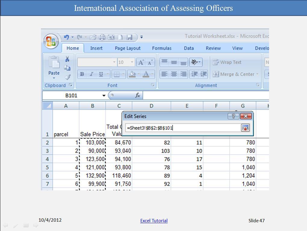
37 Let s look at several key parts of this window. 1. The Chart Data Range displays the worksheet name and the absolute references for all the data considered. It is highlighted when the dialog window first appears, which means deleting it will clear that data from the chart. 2. Data series can be added, edited or removed using the buttons found in the second area of the window. 3. Finally, labels can be selected for the horizontal axis of the chart. A scatter diagram is comprised of a series of objects (usually dots) that represent the intersection of data displayed on vertical and horizontal axes. The line chart shown earlier displayed average indices over time. The same data displayed in a scatter diagram would be more difficult to read because it would display individual cases, rather than summaries. Notice that the three windows are divided into two sections. The open part of the window allows the user to type cell references directly. If you do that, remember to make the cell references absolute, not relative. SRM 35

38 The small section to the right contains a small arrow that when pressed allows the user the point to the cells, rather than type in their references. You must enter both Series X values and Series Y values. Series X values will form the horizontal portion of the intersection and Series Y values will form the vertical. We highlighted Sale Prices for the Series X values and Ratios for the Series Y values. SRM 36

39 SRM 37

40 In just a few steps and a relatively short time, I produced a scatter chart. It is admittedly crude, but shows the relationship between ratios and selling prices. The chart can be changed to accommodate reporting needs and preferences. Under the Chart Layouts group of the Design tab is a drop down selection of pre-designed layouts. The chart will be changed immediately upon selection of any one of these items in our case layout 9. Chart and axis titles are added as placeholders. Additional gridlines have been added. A linear regression line along with the regression formula and the R 2 indicator have also been added. SRM 38

41 Axis Title Excel Tutorial Chart Title y = -7E-05x R² = , , ,000 Axis Title Series1 Linear (Series1) All of these can be changed. I would begin by deleting the legend. It adds noting to the chart and takes up viewing real estate. Next, I would make the Chart and Axis titles more meaningful. Most parts of the chart are themselves objects and the user can access their characteristics by clicking on them. Clicking on each of the titles allows the user to erase what is there and replace it with appropriate text. SRM 39

42 Even the regression data can be moved to a part of the chart that makes it more readable. For the vertical and horizontal axis, the user can select whether to display no grid lines, only major gridlines, only minor gridlines or both major and minor gridlines. These are accessed from the Axis group of the Layout tab. Much more can be done to the chart to reflect the user s taste and reporting preferences. SRM 40

43 Right clicking on the data points within the chart will bring up a dialog box that contains a number of options. You should look at the options available, apply several to gain some perspective on what they do and develop your own style preferences. Each of the axes can be adjusted according to the user s preference. Tip Any changes that you make to the worksheet data after the chart is created are instantly shown in the chart. When your chart looks just the way you want it to, it's easy to add it to a PowerPoint presentation so that everyone can see it. And if the chart data changes after you add the chart to PowerPoint, don't worry. Changes to the chart data in Excel are updated in the chart in PowerPoint as well. Here is how it works. Copy the chart in Excel. Open PowerPoint Paste the chart on the slide you want it. In the chart's lower-right corner the Paste Options button appears. Click the button. You'll see that Chart (linked to Excel data) is selected. That ensures that any changes to the chart in Excel will automatically be made to the chart in PowerPoint. Now you are ready to present your chart. SRM 41

44 Sorting Data in Excel The ability to sort is very important for analysis and manipulation of data. You can sort data by text (A to Z or Z to A), numbers (smallest to largest or largest to smallest), and dates and times (oldest to newest and newest to oldest) in one or more columns. You can also sort by a custom list (such as Large, Medium, and Small) or by format, including cell color, font color, or icon set. Most sort operations are column sorts, but you can also sort by rows. Excel will attempt to sort the entire range of data selected. This is very important from the standpoint of data integrity. In our sample dataset, if you were to sort only part of the data, some of the fields would no longer match the parcel on which they were originally recorded. If you attempt to sort a single column of data, Excel gives this warning. As you will see, it is also important to include column headings in the selection range. This helps you identify the column(s) to be used for sorting. When you reapply a sort, different results appear for the following reasons: Data has been added, modified, or deleted to the range of cells or table column. Values returned by a formula have changed and the worksheet has been recalculated. Tip: Selecting all the data on a worksheet can be accomplished easily. Holding down the control key (Ctrl) and striking the Home key will place the cursor in the upper left corner cell of the worksheet (A1). Then by holding down both the control (Ctrl) and shift keys SRM 42

45 and then striking the End key, the cursor is move to the lower right cell containing data and all the data is highlighted. Sort text First, select the range of data to be sorted. This will open a dialog box containing selections of Column, Sort on and Order. The Column drop down menu will contain the column headings if they have been included in the selected data range. The Sort on drop down menu allows the user to indicate whether the sort will be based on cell values, cell color, font color or cell icons. Finally, the Order drop down menu allows the user to indicate the direction of the sort: To sort in ascending alphanumeric order, click Sort A to Z. To sort in descending alphanumeric order, click Sort Z to A. To reapply a sort after you change the data, click a cell in the range or table, and then on the Data tab, in the Sort & Filter group, click Reapply. Issue: Check that all data is stored as text If the column that you want to sort contains numbers stored as numbers and numbers stored as text, then you will receive the Sort Warning message shown above. To format all of the selected data as text, on the Home tab, in the Font group, click the Format Cell Font button, click the Number tab, and then under Category, click Text. SRM 43

46 Sort numbers Sorting numeric data follows the same routine, except the Order drop down menu lists Smallest to Largest and Largest to Smallest instead of A to Z and Z to A. As before, make sure all the data in the sort column is numeric to avoid any problems with the sort. Sort dates or times Sorting by dates or times follows the same routine, but this time the Order drop down menu lists Oldest to Newest or Newest to Oldest. Issue: Check that dates and times are stored as dates or times If the results are not what you expected, the column might contain dates or times stored as text and not as dates or times. For Excel to sort dates and times correctly, all dates and times in a column must be stored as a date or time serial number. If Excel cannot recognize a value as a date or time, the date or time is stored as text. NOTE If you want to sort by days of the week, format the cells to show the day of the week. If you want to sort by the day of the week regardless of the date, convert them to text by using the TEXT function. The Sort dialog box allows you to sort several different columns in the same routine. For example, you could sort by Neighborhood and Sale Price. You can even change the sort order for each column. Neighborhood can be sorted from A to Z and Sale Price can be sorted from Largest to Smallest. This will allow the user to pick out the highest sale price for each neighborhood. Keep in mind the sort is hierarchical, meaning Excel will sort everything by one sort level before proceeding to the next. At some point in adding sort levels, you will reach a point when the product of the sort is meaningless. For example, if we were to add Total Acres to this sort routine, Excel would sort first by Neighborhood; then within Neighborhood it will sort by Sale Price; finally, for every matching Sale Price, it will sort by Total Acres. You can see the only condition under which the third level of sorting would apply is when two or more parcels within SRM 44

47 the same Neighborhood sell for the exact price and have different acreages. The chances of that happening and therefore reaching that third sort level are very slim. SRM 45

48 Filtering Filtered data displays only the rows that meet criteria that you specify and hides rows that you do not want displayed. After you filter data, you can copy, find, edit, format, chart, and print the subset of filtered data without rearranging or moving it. You can also filter by more than one column. Filters are additive, which means that each additional filter is based on the current filter and further reduces the subset of data. The Filter function is found in the Sort & Filter group on the Data tab. Before selecting the Filter, select the data that is to be filtered. Clicking on the filter will cause a drop down icon to appear in the bottom right corner of the top cell of each filtered column. When that icon is clicked, a dialog box appears that allows the user to adjust the filter. For example, if all the data is selected in our sample dataset, the filter is selected and the icon on the Style column is clicked, the dialog box looks as follows: Assuming there are style codes 1 through 15, this shows us that not all those codes are represented in our dataset. If we want to view only those records in style code 2 we 1. Click on the Select All check box to unselect all SRM 46

49 2. Click on the check box next to 2 to show only style code 2 parcels Now the only style that appears is 2 and the icon in the top cell of that column has changed from to indicating the use of a filter. NOTE When you use the Find dialog box to search filtered data, only the data that is displayed is searched; data that is not displayed is not searched. To search all the data, clear all filters. Additional filters can be added just as layers were added to a sort routine. For example, assume that after filtering for style 2 parcels, you wanted to look at sales of two bedroom homes. Adding that filter is as simple as moving to the column headed Bedroom, clicking on the filter and selecting only 2 from the available codes. When you do that, the number of visible rows is reduced. What is left are parcels that satisfy both filters at the same time. There may be parcels in the original dataset that have two bedrooms, but are a different style. In the same way, there may be style 2 parcels that have more than two bedrooms. None of those are visible in the filtered dataset. Notice something else in the slide: calculations were entered at the bottom of the Sale Price column reflecting the Average, Maximum and Minimum. The results of those calculations did not change with the filters. It is very easy to look down the Sale Price column and note that neither the maximum nor the minimum values match those of the calculations. SRM 47

50 Using the Show Formulas option in the Formula Auditing group of the Formulas tab reveals that the calculations are based on all rows 2 through 101 of the original dataset. Removing a filter and restoring the dataset to its original state is easy. 1. Return to the filtered column and click on the icon in the top cell. 2. Locate the selection entitled Clear Filter From followed by the column heading 3. Click on that selection The filter(s) applied to that column will be removed immediately. There are many other ways of using filters. For example, more than one of the items can be selected from a group. We could have selected style 4 and 9 instead of just style 2. You can copy the result of a filter to another worksheet. At that point, calculations become meaningful for that data segment alone. SRM 48

51 PivotTable reports in Excel 2007 Your worksheet has lots of data, but do you know what the numbers mean? Does your data answer all your questions? PivotTable reports can help to analyze numerical data and answer questions about it. In seconds you can ask questions, see the answers. With PivotTable reports, you can look at the same information in different ways with just a few mouse clicks. Imagine an Excel worksheet of sales information on multiple parcels. A PivotTable report turns all that data into small, concise reports that tell you exactly what you need to know. Before you start to work with a PivotTable report, take a look at your Excel worksheet to make sure it is well prepared for the report. When you create a PivotTable report, each column of your source data becomes a field that you can use in the report. Fields summarize multiple rows of information from the source data. The names of the fields for the report come from the column titles in your source data. Be sure that you have names for each column across the first row of the worksheet in the source data. The remaining rows below the headings should contain similar items in the same column. For example, text should be in one column, numbers in another column, and dates in another column. In other words, a column that contains numbers should not also contain text, and so on. Finally, there should be no empty columns within the data that you are using for the PivotTable report. We also recommend that there be no empty rows; for example, blank rows that are used to separate one block of data from another should be removed. When the data is ready, place the cursor anywhere in the data. That will include all the worksheet data in the report. Or select just the data you want to use in the report. Then, on the Insert tab, in the Tables group, click PivotTable, and then click PivotTable again. The Create PivotTable dialog box opens. Select a table or range is already selected for you. The Table/Range box shows the range of the selected data. New Worksheet is also selected for you as the place where the report will be SRM 49

52 placed (you can click Existing Worksheet if you don't want the report placed in a new worksheet). This is what you see in the new worksheet after you close the Create PivotTable dialog box. On the left side is the layout area ready for the PivotTable report, and on the right side is the PivotTable Field List. This list shows the column titles from the source data. As mentioned earlier, each title is a field: parcel, Neighborhood, and so on. You create a PivotTable report by moving any of the fields to the layout area for the PivotTable report. You do this either by selecting the check box next to the field name, or by right-clicking a field name and selecting a location to move the field to. If you have worked with PivotTable reports before, you may wonder if you can still drag fields to build a report. You can. Tip If you click outside of the layout area (of a PivotTable report), the PivotTable Field List goes away. To get the field list back, click inside the PivotTable layout area or report. Now you are ready to build the PivotTable report. The fields you select for the report depend on what you want to know. SRM 50

53 Let's start with finding the average selling price by style. To get the answer, you need data about the style. So select the check box in the PivotTable Field List next to the Style field. You also need data about Sale Price, so select the check box next to the Sale Price field. Notice that you don't have to use all the fields on the field list to build a report. When you select a field, Excel places it in a default area of the layout for you. You can move the field to another area if you want to. For example, when you select Style, it is moved to the Values section and displayed as. Notice to the left of the Pivot Table Field List dialog box there is a partial table being constructed interactively. At this point it displays one label Sum of Style and one amount 411. Clicking the arrow on the right side of that image causes a dialog box to appear with several choices including one to Move to Row Labels, which is where we want this field. Upon selecting the Move to Row Labels option two things occur. The label Style is moved to the Row Labels section of the dialog box and the partial table to the left has changed. It now has a label Row Labels with numbers below it and a label Grand Total below that. These numbers represent each of the unique values for Style found in the range of data selected for the pivot table. Since we want to display the average Sale Price by Style, we select the Sale Price field. It is moved into the Values section with the Sum notation and the pivot table now has values under a label Sum of Sale Price. Sum is the default setting. There are two approaches to changing that. You can select value Field Settings from the dialog box that appears after clicking the arrow to the right of Sum of Sale Price in the Values section or in the ribbon at the top of the page. SRM 51

54 Either of these approaches causes another dialog box to appear with a list of options. Selecting Average and clicking OK causes the label in the pivot table to change from Sum of Sale Price to Average of Sale Price and the numbers under that label to change also reflecting the average by style. Adjusting the Field Settings can change the pivot table to show the number of sales, the maximum sale price, the minimum sale price or the standard deviation. Another field can be added to the Column Labels section to show Average Sale Price by Style and some other field. For example, you can add Bedrooms as a column and show the Average Sale Price by Style and Bedroom count, or change the Field Settings to Count and see how many sales occur in each combination of Style and Bedroom count. The data in the pivot table can be formatted like any cell in a worksheet. Highlight the cells to be formatted alike and right click the mouse. Select Format Cells and adjust the format to personal preference. Notice there are icons next to the row labels and column labels. These allow you to adjust the pivot table by limiting the rows or columns that are shown. SRM 52

55 This tutorial is an attempt to highlight some of the functionality available in Excel and provide you the user with some of the skills you will need to take IAAO s advanced mass appraisal courses. SRM 53

56 Comp Sheet Defending values of residential property is best accomplished through the use of a comparable sales sheet, but this presents the problems of selecting the appropriate sales and then adjusting the sales for differences between the sales chosen and the subject property. These will be addressed by building a comp sheet in such a way that the user can determine how sales will be selected and the final market value estimate determined. Copy the following variables to the Comp Sheet worksheet. Remember to just paste the values to avoid confusion created by the underlying formulas on other worksheets. Parcel Sale Year Sale Month Sale Price MCAP NBHD Subdiv Land Size Building Size Year Built MS Style Full Baths Half Baths Bedrooms Condition Quality Walls Age Cost Leave two columns blank and build the structure for our comp sheet beginning with the third column following our data. Parcel Sale Year Sale Month MCAP Subdiv Land Size SFLA Age Quality Condition Bedrooms Full Baths Half Baths Cost Adj Est Market Subject Sale 1 Sale 2 Sale 3 Sale 4 Sale 5 SRM 54

57 Est The premise of the sales selection routine is twofold: that the analyst wants sales that have the same characteristics as the subject and that he or she should have the capability of determining what variables are most important in establishing comparability. The most comparable sale is one whose characteristics exactly match that of the subject, but that is only possible when the subject is one of the candidate sales. Otherwise that analyst is required to select among sales whose characteristics vary from one another and the subject in different ways. One of the ways of establishing the relative comparability of one property characteristic over another is through weighting the differences. For numeric variables such as improvement size (SFLA), a weight is applied to the difference between the value of the variable for the subject and that of a comparable sale property. For some variables such as neighborhood the question to be asked is not how much the sale property differs from the subject but whether it does. If the value of the variable for the sale is the same as that of the subject no weight is applied or a weight of 0 is applied. When the values are different, in other words in our example the sale lies outside of the subject s neighborhood, a weight is applied. When all the weights for a sale have been calculated they are summed and all the candidate sales are sorted by their weights. Those with the smallest weights are considered most comparable to the subject since their set of characteristics is closer to that of the subject property. Under the comp sheet template list a set of property characteristics and a list of starting weights. We then construct a formula that calculates the weights for each sale based on that weight list. The more characteristics that are listed the more complex the formula becomes. Item Weights Sale Date 60 Subdiv 500 Land Size 0.1 SFLA 0.25 Age 50 Quality 100 Condition 100 Bedrooms 100 Full Baths 100 Half 50 Baths =(((($W$3-B2)*12)+$W$4-C2)*$W$20)+ IF(G2<>$W$6,$W$21,0)+ (ABS($W$7-H2)*$W$22)+ (ABS($W$8-I2)*$W$23)+ (ABS($W$9-R2)*$W$24)+ IF($W$10<>P2,$W$25,0)+ IF($W$11<>O2,$W$26,0)+ IF($W$12<>N2,$W$27,0)+ IF($W$13<>L2,$W$28,0)+ IF($W$13<>M2,$W$29,0) SRM 55

58 time. There are ten variables used in this selection routine and we will take them one at a (((($W$3-B2)*12)+$W$4-C2)*$W$20) Sale date can be represented in several ways. Here it is translated into months before a weight is applied. $W$3 is used to reference the subject year. This should be the year of the appraisal date, just as $W$4 should be the month of that same date. Notice that the sale year is subtracted from the appraisal year and then multiplied by 12. That is added to the difference between the appraisal month and the sale month; and that sum is multiplied by the listed weight. IF(G2<>$W$6,$W$21,0) A conditional statement is used to determine whether the Subdiv variable for the sale is different than that of the subject property. If the sale property is not located in the same subdivision as the subject property it is assigned the weight at $W$21, otherwise it is given a weight of 0. (ABS($W$7-H2)*$W$22) The land size for a particular sale property may be either larger or smaller than the subject. All the analyst cares about is how close it is to the subject s size, so the absolute difference between them is used to establish the weighting. If that was not done, a negative weight on one variable may offset a positive weight on another, skewing the results. $W$7 represents the land size for the subject; H2 is the land size of the sale property; and $W$22 is the weight to be applied to the absolute difference. (ABS($W$8-I2)*$W$23) The size of the dwelling, represented here as SFLA (Square Feet of Living Area), is treated in the same way as the land size variable, with the absolute difference being weighted. (ABS($W$9-R2)*$W$24) The absolute difference between the age of the subject parcel and each sale is also weighted in a similar fashion. The remaining five variables in the list are weighted according to whether their value exactly matches that of the subject property. If they exactly match the value of the subject property their weight is 0, otherwise they receive the weight shown on the list. Comparability This method defines comparability in terms of the relative value of the weight. Therefore the most comparable properties are going to appear in the first rows of our worksheet when they are sorted in ascending order based on weight. That allows the user to construct the comparable sales form using references to variables in the first few rows. Some jurisdictions prefer that the subject property not be used as its own comparable when it has sold recently. Assuming it will pull itself as the most comparable sale, our comparable sale form begins on row 3, instead of row 2. In a jurisdiction where there is either no or the opposite preference, this template can be changed to begin with row 2. SRM 56

59 Setting selection weights is an iterative process involving the judgment of the analyst regarding comparability. The analyst will go through a process of setting weights, sorting the sales and reviewing the resulting comp sheet to determine whether it reflects the degree of comparability he or she wants. This process is repeated as many times as it takes to achieve a level of comparability desired by the user. Weights of variables are increased or decreased to alter the representation of that variable in relation to the other variables. For example, the Sale Date weight might be increased to bring in more recent sales. On the other hand, SFLA may be more important than sale date and its weight can be changed to reflect that. Market Estimate One of the characteristics all the sales in our sample share is a cost estimate. This was previously calculated in a similar manner for all parcels such that two parcels having the same characteristics will have the same cost estimate. Therefore, the cost estimate will be used to adjust the sales to the subject. The cost estimate of the sale property will be subtracted from that of the subject and the difference will be added to the adjusted selling price. That formula for Sale 1 is shown below. =($W$15-X15)+X5 If there is no difference in cost, the amount of adjustment will be 0. As the characteristics of the sale property differ to a larger extent from the subject the difference in cost will increase, assuming those differences affect cost. Finally, the adjusted selling prices must be aggregated in some way to estimate the value of the subject property. In this case, the formula used calculates the average of the adjusted selling prices, but the user could easily change that to the Median or some other calculation. Direct Market Another approach to estimating market value and/or providing a means of adjusting sales is through the use of multiple regression analysis. That functionality is available in Excel through Data Analysis on the Data ribbon. (If that option does not appear on the Data ribbon, follow the instructions in the Appendix to make it available.) The end product of this process will be a set of value estimates that should be tied to parcel numbers for ease of identification. The regression model will require the input of a dependent variable and one or more independent variables. That will be made easier if all those items are aggregated into a single place on the worksheet. To that end, copy the following variables to a separate part of the Comp Sheet worksheet: Parcel Sale Year Sale Month MCAP Building size Year Built Condition Quality The market conditions adjusted price is an attempt to adjust the original sale prices for market changes that have occurred since the sale date. However, to further adjust the sales to a more current date and to show the application of an additional variable, we will create a SRM 57

60 variable called DOSSF (Date of Sale times Square Feet). We will use January 1, 2010 as the appraisal date and subtract the sale date for each sale parcel from that before multiplying the result by the Building Size. The appraisal date is transformed into months by multiplying the appraisal year by 12. From that is subtracted the result of multiplying the sale year by 12 and adding the sale month to that. The resulting formula is: =((2010*12)-((AG2275*12)+AH2275))*AJ2275 It has a relative format, meaning it can be copied to each parcel. Selecting Data Analysis form the Analysis tab from the Data ribbon will cause the dialogue window below to appear. Selecting the Regression option will bring up the following dialogue window: SRM 58