Isogeometric Segmentation: The case of contractible solids without non-convex edges. B. Jüttler, M. Kapl, Dang-Manh Nguyen, Qing Pan, M.

Transcription

1 Isogeometric Segmentation: The case of contractible solids without non-convex edges B. Jüttler, M. Kapl, Dang-Manh Nguyen, Qing Pan, M. Pauley G+S Report No. July

2 Isogeometric Segmentation: The case of contractible solids without non-convex edges Bert Jüttler a, Mario Kapl a,, Dang-Manh Nguyen a, Qing Pan a, Michael Pauley a a Institute of Applied Geometry, Johannes Kepler University, Linz, Austria Abstract We present a novel technique for segmenting a three-dimensional solid with a -vertexconnected edge graph consisting of only convex edges into a collection of topological hexahedra. Our method is based on the edge graph, which is defined by the sharp edges between the boundary surfaces of the solid. We repeatedly decompose the solid into smaller solids until all of them belong to a certain class of predefined base solids. The splitting step of the algorithm is based on simple combinatorial and geometric criteria. The segmentation technique described in the paper is part of a process pipeline for solving the isogeometric segmentation problem that we outline in the paper. Keywords: Isogeometric analysis, coarse volume segmentation, edge graph, cutting loop, cutting surface. Introduction Isogeometric analysis (IGA) is a novel framework for numerical simulation that often relies on a NURBS volume representation of the computational domain. It ensures the compatibility of the geometry description with the prevailing standard in Computer Aided Design [, ]. Additional advantages include higher rates of convergence and increased stability of the simulation results. These beneficial effects are due to the increased smoothness and the higher polynomial degrees of the functions used to represent the simulated phenomena. However, a NURBS representation of the computational domain, which is often the volume of a solid object or the volume surrounding a solid object, is not provided by a typical CAD model. In connection with the advent of isogeometric analysis, several authors presented algorithms for creating a NURBS volume representation from a given CAD model: Corresponding author addresses: bert.juettler@jku.at (Bert Jüttler), mario.kapl@jku.at (Mario Kapl), manh.dang_nguyen@jku.at (Dang-Manh Nguyen), panqing@lsec.cc.ac.cn (Qing Pan), michael.pauley@jku.at (Michael Pauley) Preprint submitted to Elsevier July,

3 Martin et al. [] describe a method to generate a trivariate B-spline representation from a tetrahedral mesh. First, a volumetric parametrization of the genus- input mesh by means of discrete harmonic functions is constructed. This initial parametrization is then used to perform a B-spline volume fitting to obtain a B- spline representation of a generalized cylinder. An extension of this work to more general objects (e.g. to a genus- propeller) is presented in []. Another parametrization method for a generalized cylinder-type volume is proposed in []. A NURBS parametrization of a swept volume is generated by using a leastsquares approach with several penalty terms for controlling the shape of the desired parametrization. Among other applications, this method can be used to generate volume parameterizations for blades of turbines and propellers. Xu et al. [] present a volume parametrization technique for a multi-block object. The parametrization of a single block is constructed by minimizing a quadratic objective function subject to two constraints. While one condition ensures the injectivity of the single B-spline parametrizations, the other condition guarantees C -smoothness between the blocks. Another volume parametrization method [] generates first a mapping from the computational domain, which is given by its boundary, to the parameter domain by means of a sequence of harmonic maps. The parametrization of the computational domain is then obtained by a B-spline approximation of the inverse mapping. Given a boundary representation of a solid as a T-spline surface, which is assumed to have genus zero and to contain exactly eight extraordinary nodes, the algorithm in [] constructs a solid T-spline parametrization of the volume. Further approaches to volume parametrization are described in [ ]. Since many of the existing methods for (NURBS) volume parametrization are restricted to simple objects (cf. []) or to decompositions of more complex objects into simple ones, an algorithm for splitting a solid represented by a CAD model into a collection of simpler solids is of interest. In particular, decompositions into solids that are topologically equivalent to hexahedra or tetrahedra are desirable, since these objects can be easily parametrized by tensor-product NURBS volume patches. The decomposition of a convex polyhedron into a collection of tetrahedra is a wellstudied problem [, ]. A tetrahedralization of a convex polyhedron can be also generated by barycentric subdivision (cf. []), which can be applied to any connected polyhedral complex, see []. For general polyhedra, several methods for decomposing them into smaller convex polyhedra have been studied, e.g. [ ]. In contrast to the convex case [], it is not always possible to obtain a tetrahedralization without adding new vertices, cf. [].

4 A well-established approach to the decomposition of a CAD model is the use of the geometric information that is provided by its features (e.g. sharp edges). Chan et al. [] describe a volume segmentation algorithm that can be used for prototyping applications. The initial solid is repeatedly decomposed into smaller ones until all resulting models belong to a class of so-called producible solid components. It is ensured that the union of the constructed solids represents again the initial object. Other feature-based methods that have been described in the literature, (e.g. [, ]) decompose polyhedral objects and special curved objects (i.e. objects with planar and cylindrical surfaces) into maximal volumes. In the method described in [], the maximal volumes are always convex objects, whereas in [] in some cases the maximal volumes may include objects with a few non-convex edges, too. Another approach to the segmentation of a CAD model is the representation as a hexahedral mesh with many hexahedra of approximately uniform size and shape. This is usually referred to as the problem of hex(ahedral) mesh generation. Due to the importance of hex meshes for numerical simulation, this problem has continuously attracted attention over the years. A feature-based algorithm for generating such meshes was introduced in [], consisting of the following steps. The first phase is devoted to the feature recognition, which provides a guiding frame for the decomposition of the CAD model. Secondly, cutting surfaces are constructed, which split the initial solid into hex-meshable volumes. Further examples of hexahedral meshing algorithms are described in [ ]. In contrast to these approaches, our goal is the decomposition of a CAD-model into a small number of topological hexahedra, which can be parametrized by single trivariate tensor-product NURBS-patches. More precisely, we consider the following Isogeometric Segmentation Problem: Given a solid object S (represented as a CAD model), find a collection of mutually disjoint topological hexahedra H i (i =,..., n) whose union represents S. The shape of the topological hexahedra need not to be uniform, and the hexahedra are not required to meet face-to-face, thereby allowing T-joints. However, the number n of topological hexahedra should be relatively small. Each of the topological hexahedra can be represented as a trivariate NURBS volume, which can then be used for performing a numerical simulation using the isogeometric approach. By using a small number of topological hexahedra, it is possible to exploit the regular tensor-product structure on each of them. Since the individual NURBS volumes may not meet face-to-face, advanced techniques (e.g., based on discontinuous Galerkin discretizations) for coupling the isogeometric discretization are required. In the context of IGA, such techniques are currently being investigated in []. We expect that a valid solution to the isogeometric segmentation problem can be obtained using a smaller number of topological hexahedra than the traditional hexahedral meshing. This is because

5 Original solid Hexahedral meshing # s: Isogeometric segmentation # s: Figure : An example that helps to distinguish our isogeometric segmentation (IGS) problem from the traditional hex meshing (THM) problem. Left: An example solid with a -vertex-connected edge graph. Middle: A natural decomposition of the example solid as a solution to the THM problem; we believe that this is the coarsest decomposition that does not possess T-joints. Right: A segmentation of the example solid as a solution to our IGS problem; we note that the segmentation admits T-joints. the individual hexahedral elements do not need to meet face-to-face (cf. Figure ), and the shape of NURBS volumes is much more flexible than that of traditional hexahedral elements. For instance, a ball can be represented exactly with only seven tri-quartic NURBS volumes, but its (approximate) representation as a hexahedral mesh may require a large number of elements, depending on the required geometric accuracy of the hexahedral mesh. It is difficult to quantify the savings in the number of hexahedral elements, since this depends also on the required geometric accuracy of the hexahedral mesh. The reduction of the number of elements, however, is not the sole advantage of using isogeometric segmentation and isogeometric analysis. The resulting collection of trivariate NURBS volumes can be used to obtain a traditional NURBS-based CAD model. (This CAD model could be constructed from those boundary surfaces of the hexahedral NURBS volumes which lie on the boundary of the solid.) This results in a CAD model and a computational model which are consistent with each other. This advantage is at least as important as the reduction in the number of hexahedra, since it supports a higher level of interoperability of the various design and analysis tools, in particular in connection with shape optimization. We present a new splitting algorithm that can be seen as the first step towards solving the IGA segmentation problem for general solid objects. In this paper we shall consider

6 genus-zero objects with only convex edges; the extension to more general solids is discussed in a follow-up paper []. Future work will also address decompositions that allow a more direct coupling of the various subdomains. More precisely, the algorithm presented in the paper is part of a process pipeline for solving the isogeometric segmentation problem stated above. An outline of the entire pipeline will be given in the final section of the paper. The splitting algorithm is based on the edge graph of the given solid. We repeatedly decompose the edge graph into smaller sub-graphs, until all sub-graphs belong to a certain class of predefined base solids. The base solids can then be represented by a collection of topological hexahedra. We introduce a cost function for identifying the best possible splitting in each step. This selection by the cost function is based on simple combinatorial and geometric criteria. In principle, exploring all possibilities would allow to find the decomposition with the smallest number of hexahedra. In practice, however, it is preferable to find a solution that is close to optimal with less computational effort. Several examples will demonstrate that this aim is achieved by the splitting algorithm. The remainder of the paper is organized as follows. We introduce some basic definitions in Section. In particular, we explain the concept of the edge graph of a solid and state the required assumptions. Section describes the main idea of our segmentation algorithm, which is based on the edge graph of the solid. Section provides a theoretical justification for the proposed approach. In order to obtain a near-optimal result, we introduce in Section the concept of the cost function, which provides the possibility to automatically guide the segmentation steps based on simple combinatorial and geometric criteria. Section presents decomposition results for different example solids. An outline of the entire process pipeline for solving the isogeometric segmentation problem is given in Section. Finally, we conclude the paper.. Solids and edge graphs We consider a solid object S in boundary representation (BRep). It is defined as a collection of edges E = {e,..., e m }, faces F = {f,..., f n }, and vertices V = {v,..., v l }. The faces are joined to each other along the edges, and the edges meet in vertices. The faces are generally free-form surfaces (e.g., represented as trimmed NURBS patches), and the edges are free-form curves (e.g., represented by NURBS curves). By considering only the edges and the vertices, we obtain the edge graph G(S) of the solid. Consider the normal plane of an edge at an inner point. It intersects the two neighboring faces in two planar curve segments, and it contains the two normal vectors n, n of these faces. Let t, t be the two tangent vectors of the planar curve segments (oriented such that they point away from the edge). If n, t do not separate n, t, then the edge is said to be convex at this point. An edge that is convex at all inner points is convex, otherwise it is non-convex. Throughout the paper we make the following assumptions. A. The solid S is contractible, i.e., it is homeomorphic to the unit ball. Consequently, neither voids (i.e. hollow regions within the solid) nor tunnels (holes through the solid) are present.

7 A. All edges are convex, any two vertices are connected by at most one edge, and all vertices of any face are mutually different. The first assumption implies that the edge graph is a planar graph, in the sense that it can be embedded into the plane such that the embedded vertices are mutually different and the embedded edges intersect each other in vertices only. Note that assumption A does not imply that the solid S is convex itself, due to the presence of free-form boundaries. Solids not satisfying these assumptions can be dealt with by an extension of the methods presented in this paper. This will be the topic of the follow-up paper []. The construction of the edge graph from a given D geometry will not be discussed in this paper. In most cases, the edge graph of the solid can be derived directly from the CAD data. For a solid that is represented by a triangular mesh, the edge graph can be generated by detecting the sharp edges of the triangular mesh, possibly followed by cleaning and repairing steps. We recall the following definition []: Definition. An (edge) graph G is said to be k-vertex-connected if it has at least k + vertices and it remains connected after removing any set of k vertices. We will consider solids that satisfy the following additional assumption (again, the more general case will be addressed in future work): A. The edge graph is -vertex-connected. According to the Steinitz Theorem in polyhedral combinatorics, any planar graph that satisfies Assumption A can be obtained from the edges and vertices of a convex polyhedron, and the graphs satisfying Assumption A are therefore called polyhedral graphs [, ]. Figure shows three examples of solids, their edge graphs and the associated planar embeddings. In these examples, which will be used throughout this paper, the boundary faces are represented as triangular meshes, and the edge graphs were generated by an edge detection method. If two vertices or edges belong to the same face, then we say that they share a common face. For future reference we state the following observation. Lemma. The edge graph is -vertex-connected if and only if any two non-neighboring vertices of any face do not share another face. proof. We show that the negations of the two statements are equivalent. First we consider an edge graph that possesses a face f k with two non-neighboring vertices v i, v j sharing this face and another face f l, cf. Figure, left. The two vertices can then be connected by two additional edges in the graph (shown in blue), one within each of the two faces. The loop formed by these two edges splits the edge graph into two disjoint subsets. Consequently, after removing the two vertices, the graph splits into two sub-graphs, thereby contradicting the assumption that it is -vertex-connected.

8 f l v i v j Solid Solid Solid Figure : First row: Three solids with sharp edges. Second row: The associated edge graphs with only convex edges. Third row: The corresponding planar embeddings. v i G f k v j G Figure : Left: An edge graph that possesses a face with two non-neighboring vertices sharing two faces is not -vertex connected. Right: A non--vertex-connected graph possess a face with two non-neighboring vertices sharing more than one face.

9 hexahedron () tetrahedron (TE) pyramid (PY) prism () Figure : Four types of base solids. Each base solid can be represented by a mesh of topological hexahedra. On the other hand, consider an edge graph that is not -vertex-connected. Clearly, it is at least -vertex-connected; otherwise Assumption A would be violated, since the vertex whose deletion splits the graph would appear in the same face twice. Consider the situation in Figure, right. Deleting the two vertices v i and v j splits the graph into two disjoint components G and G. The dashed lines represent edges that may or may not be present. Even when connected by an edge, the two vertices v i and v j are non-neighboring vertices of the outer face but they share more than one face. However, v i and v j cannot be connected by more than one edge, because of Assumption A. Thus, if a graph is not -vertex-connected then there exist two non-neighboring vertices of a face that share more than one face.. Solid splitting algorithm We say that a solid is a topological hexahedron if its edge graph is equivalent to the edge graph of a cube and if all edges are convex. Our goal is to generate a decomposition of the given solid into a collection of such topological hexahedra. In order to achieve this goal, we split the solid and its edge graph into two solids with smaller edge graphs. More precisely, the edge graphs of the two solids contain only vertices of the original edge graph, but they may possess additional edges. We apply this decomposition step repeatedly to each resulting solid and associated edge graph, until we arrive at a sufficiently simple solid, which we will call a base solid. In this paper we use four types of base solids, see Figure. In addition to topological hexahedra, we also allow topological tetrahedra, pyramids, and prisms. These are defined in the same way as topological hexahedra. In principle, using only tetrahedra would be sufficient, since each tetrahedron can be split into four topological hexahedra. In order to obtain a small number of topological hexahedra, however, it is advantageous to consider hexahedra as base solids, too. Otherwise, even a solid that is already a topological hexahedron will be split into six tetrahedra, resulting in hexahedra. Finally, we also added pyramids and prisms as base solids in order to simplify the presentation of the examples below. Before describing our approach in more detail, we introduce several definitions. Definition. An auxiliary edge is an additional edge in the edge graph that connects two

10 Figure : Left: The initial edge graph of a solid. Center: A valid cutting loop with one auxiliary edge and three existing edges (red edges). Right: The resulting two smaller edge graphs with the cutting surface. non-adjacent vertices on a face. Any two non-adjacent vertices of a face can be joined by an auxiliary edge. A cutting loop is a simple closed loop of existing or auxiliary edges of the edge graph, such that no two edges of the loop belong to the same face. A cutting surface is a multi-sided surface patch whose boundary curves are the existing or auxiliary edges of a cutting loop. It is a newly created surface patch inside the solid. We say that the cutting surface is well-defined if it can be used to split the given solid object into two smaller solids. Due to the assumptions regarding the cutting loop, a well-defined cutting surface for each cutting loop exists. Indeed, the tangent planes of the cutting surface can be chosen such that the solid is subdivided into two sub-solids by the cutting surface. However, if two neighboring edges of the cutting loop shared a common face, then the tangent plane of the cutting surface at the corresponding common vertex would touch this face and the cutting surface would not be well-defined. This fact motivates the requirement concerning the edges in the definition of the cutting loop. Clearly, there is always an infinite number of possible cutting surfaces for a given cutting loop. All these surface patches possess the same boundary curves. As a first example, Figure visualizes a simple edge graph of a solid with a valid cutting loop, the cutting surface and the two resulting smaller edge graphs. In order to be able to formulate our recursive splitting algorithm, we will introduce another notion. Definition. A cutting loop is said to be valid for the edge graph G of a given solid if any associated cutting surface decomposes the given solid into two smaller solids that again satisfy Assumption A. First we present a characterization of valid cutting loops. Proposition. A cutting loop is valid if and only if it contains at least three vertices and if all pairs of non-neighboring vertices do not share a face of the edge graph G. proof. If the cutting loop is valid, then each of the two edge graphs of the solids, which are obtained by splitting the given solid using an associated cutting surface, is again - vertex-connected. In these two graphs, any two vertices v i, v j of the cutting loop lie on the

11 face that corresponds to the cutting surface. According to Lemma, if the two vertices are not neighbors, then they must not share any other face of the edge graphs, since these two edge graphs are both -vertex-connected. Since all other faces of the edge graphs are (parts of) faces of the original edge graph G we conclude that all pairs of non-neighboring vertices of the cutting loop do not share a face of the original solid G. On the other hand, consider two non-neighboring vertices v and v of a face of one of the two sub-solids that are obtained after splitting. We need to show that they do not share any other face, provided that all pairs of non-neighboring vertices of the cutting loop do not share a face. If one of the two vertices v and v does not belong to the cutting loop, then this is implied by the fact that the original solid satisfies Assumption A. If both belong to the cutting loop, however, then this is exactly the condition that characterizes the cutting loop in the proposition. Based on this characterization for the validity of a cutting loop, Section will discuss the existence of a valid cutting loop in more detail. Now we are ready to formulate the solid splitting algorithm SplitSolid. The algorithm splits the edge graph of the solid into a collection of topological base solids, which correspond to hexahedra, tetrahedra, pyramids and prisms, see Figure. Each of these solids can be easily decomposed into a collection of topological hexahedra. More precisely, we obtain hexahedra for a tetrahedron, n hexahedra for a prism with a n-sided polygonal base and n tetrahedra (and hence n hexahedra) for a pyramid with a n-sided polygonal base. Algorithm SplitSolid: Splitting the edge graph of the solid : procedure SplitSolid(graph G) : if G is a base solid then : return G and/or its subdivision into topological hexahedra : else : find the set L of all possible valid cutting loops : ChooseCuttingLoop(L) : decompose G into sub-graphs G and G : return SplitSolid(G ) and SplitSolid(G ) : end if : end procedure The selection of a valid cutting loop, performed by the function ChooseCuttingLoop, will be explained in Section. Note that any edge graph with n vertices (n ), all possessing valency three, could be used as a base solid, since this polyhedron can be split into n hexahedra by midpoint An alternative way to cut a prism with n sided base, n, results in n/ hexahedra, possibly by cutting at midpoints of edges. A second alternative is to continue using SplitSolid until all prisms are reduced to triangular prisms and hexahedra, and this is what we do in the examples in Section.

12 v v v v v v v v Figure : An extended -ring neighborhood of an arbitrary vertex v having valency three. For more detail, we refer to the first case in the proof of Theorem. subdivision. In the following, this segmentation is referred to as simple decomposition. In Section, we will show that our splitting algorithm often leads to a reduced number of topological hexahedra when compared to the simple decomposition (see Table ). The following Section will also address the termination of this algorithm.. Existence of a valid cutting loop The following statements guarantee that our splitting algorithm works for all solids that satisfy Assumption A. Theorem. If the edge graph G is not the edge graph of a topological tetrahedron (which is the complete graph K ), then at least one valid cutting loop exists. proof. We distinguish between two cases. First case. We consider edge graphs where all vertices possess valency three. According to the Steinitz Theorem, these edge graphs can be obtained from a convex polyhedron with planar faces, where all vertices have valency. We may then pick one of the vertices and split the polyhedron into the tetrahedron formed by that vertex and its three neighbors and the remaining convex polyhedron. More precisely, we proceed as follows. We pick an arbitrary vertex, denoted by v, and connect the three neighboring vertices by a loop of existing and/or auxiliary edges, see Figure, left. The dashed lines represent either existing or auxiliary edges, and the red lines represent edges that may or may not exist. First we observe that at least one of the red edges must exist, since the entire edge graph does not represent a tetrahedron. Now we conclude that at least one red edge for each of the three vertices v, v, and v exists, since the graph is -connected. If for one of the three vertices a red edge would not exist, then deleting the other two vertices would split the graph into two disconnected sub-graphs. Now we assume that two of these three edges belong to the same face. We consider the situation in Figure, right, and assume that the two green edges share a face. Consequently, we can join the vertices v and v by an auxiliary edge (shown in blue) across this

13 v i v i v v v j+ v j+ v j v j Figure : A part of the -ring neighborhood of a vertex v with a valency greater than three. For more detail, we refer to the second case in the proof of Theorem. face. Deleting v would then split the graph into two disconnected sub-graphs, thereby contradicting the assumption that the graph is -vertex connected. Since the cutting loop consists of only vertices, it is automatically valid, see Proposition. Second case. We consider an edge graph G where at least one vertex has a valency greater than three. We pick one of these vertices and denote it by v. The n neighbors, where n > is the valency of v, can be connected by a closed loop of existing and/or auxiliary edges, see Figure, left. If all pairs of non-neighboring vertices of this loop do not share any face, then the same is true for the edges of the loop, and we found a cutting loop. Clearly, this loop is then also valid according to Proposition. Otherwise, if two vertices, say v i and v j share a face, then we connect them by an existing or auxiliary edge of this face and consider the loop with the vertices v i, v j and v, see Figure, right. We show that this loop is then a cutting loop. It is then automatically also valid, since it consists of only three vertices, see again Proposition. If the two dashed blue edge were on the same face, then we could draw a curve connecting v with itself that does not intersect any other edge but encircles some of the other vertices. This, however, contradicts the assumption that G is -vertex-connected, since removing v would split the graph into two disconnected components. Also, if one dashed edge, say (v, v i ), and the one blue non-dashed edge were on the same face, then we could create an auxiliary edge connecting vertex v and v j across that face. The loop formed by the two existing and auxiliary edges between v and v j then encircles some of the remaining vertices and deleting both v and v j splits the graph into two disconnected components, thus violating the assumption that the graph is -vertexconnected. Summing up, we can find at least one valid cutting loop in all cases.

14 Corollary. Any solid that is not topologically equivalent to a tetrahedron can be segmented into a collection of topological hexahedra using algorithm SplitSolid. proof. In each recursive step of the algorithm we will find at least one valid cutting loop. Moreover, the splitting step does not introduce additional vertices, and the number of vertices in the two sub-solids is always less than in the original solids. Consequently, after finitely many steps we arrive at a collection of base solids, which can then be subdivided into topological hexahedra. In particular, if we allow only tetrahedra as base solids, then we are able to decompose the edge graph of the solid into a mesh of (topological) tetrahedra without adding new vertices. This would be similar to the tetrahedralization algorithm for convex polyhedra in []. Our main goal, however, is to obtain a subdivision with a small number of topological hexahedra. This will be achieved with the help of a suitable cost function.. Cost-based splitting algorithm The procedure ChooseCuttingLoop provides a simple possibility to automatically select a valid cutting loop in the splitting algorithm. This is achieved by combining simple combinatorial and geometric criteria. Algorithm ChooseCuttingLoop: Selection of the cutting loop : procedure ChooseCuttingLoop(set L of valid cutting loops) : compute for each cutting loop λ the value ν with the help of the sequence ω : choose a cutting loop λ max that realizes the highest value ν : return λ max : end procedure Let L be the set of all possible valid cutting loops for the given edge graph G of the solid. For each cutting loop λ L, we compute a value, depending on the length and on the number of auxiliary edges of the cutting loop λ. In detail, we compute the value ν(λ) = ω n m p, where ω n is a value that depends on the length n (i.e., the number of vertices) of the cutting loop, m is the number of auxiliary edges of the cutting loop and p is the cost of introducing an auxiliary edge. As a simple extension, one might introduce additional geometry-related terms in this cost function. These terms could measure the deviation of the cutting surface from a plane, thereby encouraging planar cutting surfaces, and similar geometric criteria. Based on the cost function we establish a ranking list of the valid cutting loops. We choose a cutting loop that realizes the highest value of ν. If two or more have the same highest value, then we select one loop randomly.

15 ω ω ω ω ω p decomposition decomposition decomposition Table : Instances of possible decomposition sequences ω = (ω, ω, ω, ω, ω p), which are used for decomposing the Solid, Solid and Solid in Figure, and, respectively. We call the sequence ω = (ω,..., ω s p) for s >, which controls the cost function, the decomposition sequence. The number s specifies the maximum length of the cutting loops to be considered by the algorithm. The decomposition sequence is specified by the user in advance. Table shows three different instances of possible decomposition sequences, which we used in our examples in Figure -. In all examples, the length of the valid cutting loops was restricted to at most s =. The selection of the valid cutting loop is performed by algorithm ChooseCutting- Loop. It is useful to run SplitSolid multiple times with different random number seeds, and choose the best outcome. For the examples in Section, after several runs, the segmentations with the smallest number of hexahedra were examined and one was selected manually after visually inspecting its suitability for generating NURBS volume parameterizations. For the future we plan to automate this selection process based on parameterization quality measures. Moreover, it will be useful to incorporate an estimate of the quality of the resulting shapes into the value of a cutting loop and this is a subject of our ongoing research. We briefly discuss an upper bound on the complexity of ChooseCuttingLoop. The loops containing a given edge can be enumerated in order of increasing length using Yen s algorithm [] in time O(l ) per loop, where l is the number of vertices. The time required to check that a loop is valid and compute its value is small compared to l. Therefore, if K is the number of loops to be examined, the complexity is O(l K). To find an upper bound for K, suppose that there are m edges, the maximum valency of any vertex is v max, the maximum number of vertices on any face is d max and the maximum length of loops considered is s. Then, beginning with an edge and constructing a loop by adding one new (existing or auxiliary) edge at a time, we see that K = O ( m (v max d max ) s ). This estimate is very pessimistic, and does not consider that a loop must close up. Furthermore, depending on the choice of the decomposition sequence ω, the enumeration of loops may sometimes be stopped early when it can be guaranteed that no longer loops can have higher scores than the current best. We can also look at the number of (recursive) calls to SplitSolid in terms of s and l. If l = then the solid is a tetrahedron and only one call to the function is required; suppose now l >. Suppose a cutting loop of length i is used, and there are j vertices on one side of the loop and k vertices on the other side. Then i + j + k = l, and the two resulting solids after the split have i + j and i + k vertices respectively. Maximizing over i, j, k defines a recursive function which provides an upper bound on the number of calls. This function can be computed exactly; asymptotically it is O( s l).

16 The solids appearing as inputs to SplitSolid at recursive depth D must have at most l D vertices; therefore the maximum recursion depth is l. The maximum vertex degree v max,d at depth D satisfies v max,d l D. It also increases by at most per step, so v max,d v max +D; combining these inequalities gives v max,d (v max +l ). The maximum number of vertices on a face d max,d is bounded above by max(d max, s). Putting together all of the above gives a pessimistic estimate for the total complexity for Split- Solid of O ( l m ((v max + l ) max(d max, s)) s ). Note m l(l ), v max < l, d max < l. Therefore, treating s as a constant, the complexity of SplitSolid is polynomial in l. As a straightforward modification of the algorithm, one might combine two or even more splitting steps and consider the total costs, in order to obtain a globally optimal splitting of a solid. However, the number of possible cuts grows exponentially with the number of cutting steps that are considered simultaneously.. Examples We present several examples of possible volume segmentations for different geometries. First, we apply our approach to the three solids shown in Figure to study the effect of different choices for the decomposition sequence. Further examples are then investigated to observe the geometric aspects of the segmentation and the consequences of different preprocessing strategies. Solids. (See Figure -). As first examples, we choose the three solids from Figure as starting point of the segmentation. Each of them is decomposed with the help of the cost-based splitting algorithm by using the three decomposition sequences ω given in Table. Figure depicts the initial geometries, the resulting edge graphs and the corresponding planar embeddings. The resulting decompositions of the edge graphs are shown in Figures -. In each step of the splitting algorithm, a cutting loop was automatically selected (red loop), which consists of existing (dashed) and auxiliary edges (non-dashed). Table summarizes the resulting number of topological hexahedra for the different decompositions of the three solids, compared with the corresponding simple decompositions where possible. In all cases, the third decomposition sequence was the best choice for the segmentation in the sense of generating the minimal number of resulting topological hexahedra. This may be due to the fact that four-sided cutting surfaces were encouraged by this decomposition sequence. In Figure, we present the segmentation results for this decomposition sequence for the three solids. Chair stand. Now we apply our method to the chair stand shown in Figure. Our experience from the previous examples led us to conclude that Decomposition Sequence (See Table ) is a good choice for keeping the number of hexahedra in the final segmentation small. Therefore we use this sequence for the following examples. The chair stand consists of five identical pieces, and for simulation purposes it is preferable that the segmentation algorithm is applied to a single piece, so that the result

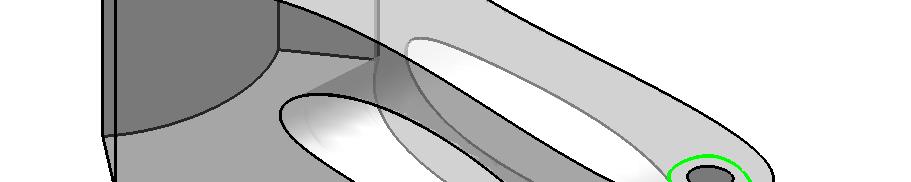
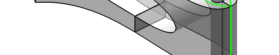
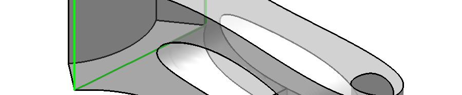
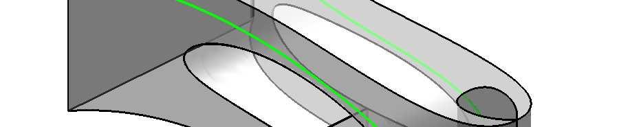
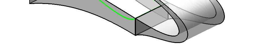
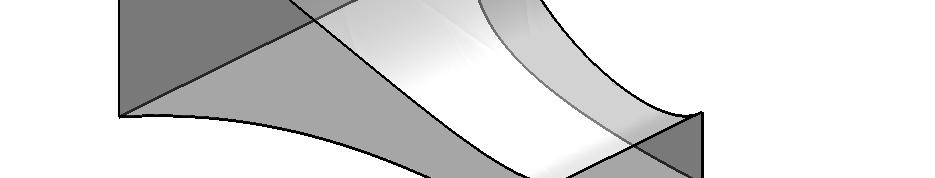
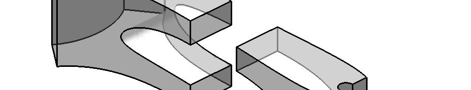
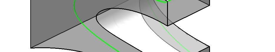
17 Solid Solid Solid simple decomposition n/a decomposition decomposition decomposition Table : Number of topological hexahedra for the resulting segmentations of the solids in Figure - for the three different decomposition sequences given in Table, compared with the corresponding simple decompositions if possible. For Solid the simple decomposition is not available, since not all vertices of its edge graph have valency three. respects the symmetry of the design. The piece has two holes in it, and our method applies only to simply connected geometries, therefore some manual preprocessing is required. We show the effects of our method in combination with several preprocessing strategies. Firstly, we try just adding internal faces as shown in Figure. We refer to this as the -cut strategy. The result is shown in Figure ; the solid is segmented into five hexahedra but the shapes are not of a good quality, being difficult to parameterize. Our second preprocessing strategy, the -cut strategy, cuts the solid into smaller pieces by making two cuts for each hole. The preprocessed solid and the results are shown in Figure. The -cut strategy results in a segmentation into hexahedra, with higher quality. Even higher quality is achieved using four cuts per hole (-cut strategy, Figure ) which results in ( ) + ( ) + ( ) = topological hexahedra but of a higher quality. (In this example, topological pentagonal prisms arise, each of which are cut into a hexahedron and a triangular prism. A smaller number of hexahedra could be achieved by inserting vertices.) Finally we try dividing the piece along its two reflection symmetries (Figure ) which results in topological hexahedra but the quality of the shapes is not as high as for the -cut strategy. Mechanical part of Zhang and Bajaj. Consider a mechanical part depicted in Figure a. The solid is similar to that considered in Zhang and Bajaj []. In a first pre-processing step, we manually cut the two cylindrical components off from the solid. As a circular face of each cylindrical component can be subdivided into five topological quads, each of the cylindrical component can be segmented into five topological hexahedra. The remaining component is a holey cube of genus which can be obtained from a cube by cutting away the intersection of the cube with two orthogonal cylinders with the same radius, see Figure b. This component consists of eight congruent pieces. As mentioned before, it suffices to only segment one piece. Our approach applied to one piece results in the decomposition depicted in Figure a. We note that out of all resulting base solids, the (only) topological hexahedron has a vertex V (see Figure a) at which two adjacent faces meet at a zero angle. The study for avoiding such a situation will be carried out in the follow-up paper []. Nevertheless, by utilizing the yet another mirror symmetry of one piece, we obtain the decomposition presented in Figure b in which the problem related to zero angles

18 disappears. Mechanical part of Yamakawa and Shimada. Another mechanical part is shown in Figure. This is based on an example from []; we have preprocessed it to cut a non-convex edge. The holes can be dealt with using a -cut, -cut or -cut strategy. (Figure shows the part preprocessed according to the -cut strategy.) Whichever choice is made, the top piece ends up being a union of topological prisms, so we only consider the base. The result for the -cut strategy is shown in Figure. Although there are just one triangular prism and two hexahedra, this segmentation is not ideal as it would be difficult to produce volume parameterizations. Figure shows the result for a -cut strategy: one of the two (identical) pieces is segmented into two prisms and a hexahedron. Thus the base of the mechanical part is segmented into a total of hexahedra. (Since a topological pentagonal prism arises, by allowing the addition of new vertices, the solid could be segmented into fewer hexahedra). Figure shows the result for the -cut strategy. One of the two nontrivial pieces is segmented into two prisms and a hexahedron. Thus the base of the mechanical part is segmented into hexahedra. The results in Figures,, support our claim that the quality of the final shapes depends on the total turning angle of the curves that are input into our algorithm. In preprocessing some solids with holes, we examined a -cut, -cut and -cut strategy, and found that the -cut strategy leads to base solids with better shape, even if the total number of topological hexahedra is higher. We believe that in the interest of high quality shapes, it is useful to ensure that there are restrictions on the total variation of the surface normal of any surface and the total turning angle of any edge, as well as the maximum ratio of the lengths of any two edges. It is also useful to incorporate geometric criteria into the value of a cutting loop, and work in this direction is ongoing.. Towards an isogeometric segmentation pipeline The work presented in this paper is the first step towards establishing a process pipeline for solving the isogeometric segmentation problem. We use this section to describe the planned workflow of the entire process. In order to illustrate the process we shall use the TERRIFIC part (data courtesy of our project partner Dr. S. Boschert / Siemens) which is one of the benchmark examples in the European project that provides some of the funding for this research, see Figure (a). The process is divided into the following steps, illustrated in Figure.. CAD model simplification and preparation. Most existing CAD models cannot be used directly, since they contain too many details or the geometric description of the boundary is too complicated. For instance, single faces of the boundary may be described by several (possibly trimmed) surface patches, and this would cause problems for the isogeometric segmentation. Consequently, it is necessary to establish a clean representation of the geometry before entering the remaining steps of the isogeometric segmentation pipeline.

19 decomposition PY - - decomposition decomposition Figure : Three different decomposition results (i.e. the planar embeddings of the resulting edge graphs) for Solid, see Figure, by using the three different decomposition sequences ω given in Table. The red loops in each step are the selected cutting loops with the existing (dashed) and the auxiliary edges (non-dashed).

20 decomposition TE TE TE PY TE decomposition TE decomposition Figure : Three different decomposition results (i.e. the planar embeddings of the resulting edge graphs) for Solid, see Figure, by using the three different decomposition sequences ω given in Table. The red loops in each step are the selected cutting loops with the existing (dashed) and the auxiliary edges (non-dashed).

21 - decomposition - decomposition - decomposition Figure : Three different decomposition results (i.e. the planar embeddings of the resulting edge graphs) for Solid, see Figure, by using the three different decomposition sequences ω given in Table. The red loops in each step are the selected cutting loops with the existing (dashed) and the auxiliary edges (non-dashed).

22 Solid Solid Solid Figure : Segmentation results for the three solids from Figure for the third decomposition sequence (decomposition ) given in Table. The associated cutting surfaces for a model are drawn with the same color. Figure : A chair stand, defined by a boundary representation. The stand is comprised of five identical pieces. One fifth of the chair stand is extracted for isogeometric segmentation. The piece has been preprocessed by adding interior faces to make it simply connected. Our approach relies entirely on triangulated CAD models, as this data format provides a very versatile representation of shapes. After a manual simplification, we triangulate the CAD model and use the triangulation to identify the faces of the CAD model by an automatic segmentation procedure. Each of the faces is then approximated by a single trimmed NURBS patch using well-established methods for geometry reconstruction. We obtain a representation of the object s boundary as a collection of trimmed NURBS surface, where each face is described by exactly one surface.. Adding auxiliary edges to obtain contractible solids with -vertex-connectivity. After creating and analyzing the edge graph, we cut the solid by auxiliary cutting surfaces in order to obtain contractible solids. Moreover, we add auxiliary edges (which have to be considered as non-convex edges) in order to make the edge graph -vertexconnected. This step is not yet automated. Some experimental results for different strategies to choose the auxiliary cutting surfaces have been described in the previous section.

23 Figure : A segmentation of the stand piece, beginning with the solid preprocessed by the -cut strategy (Figure ). In this case, the solid is segmented into topological hexahedra. Figure : Left: manual preprocessing of the stand piece using the -cut strategy. Right: segmentation of the two non-hexahedral pieces.. Dealing with non-convex edges. In the next step we eliminate the non-convex edges by cutting the solid using suitable cutting surfaces. This step is discussed in more detail in a follow-up paper [].. Subdividing a contractible solid with only convex edges. At this stage, the original

24 Figure : Left: manual preprocessing of the stand piece using the -cut strategy. Right: segmentation of the two classes of non-hexahedral pieces. solid has been segmented into a number of contractible solids with only non-convex edges. We use the techniques developed in the present paper to subdivide them automatically into base solids. Each base solid is then further subdivided to topological hexahedra.. Creating trivariate NURBS patches. Finally we create NURBS volume parameterizations for each of the resulting topological hexahedra. Currently we use a simple method which is based on trivariate Gordon-Coons parameterizations and NURBS fitting. More sophisticated techniques have been studied in the literature, see [] and the references therein. There are several geometric challenges in the process pipeline which will benefit from a more detailed investigation. These include improved techniques for segmenting the faces of the given solid, in particular if blending surfaces are present, advanced selection strategies for cutting loops, which take the shape of the resulting sub-solids into account,

25 Figure : A segmentation of the stand piece, preprocessed by cutting along symmetries. This segmentation yields two triangular prisms and two hexahedra. Thus, each quarter of the stand is decomposed into hexahedra. (a) (b) Figure : (a): The mechanical part of Zhang and Bajaj. (b): a holey cube of genus, the remaining component of the mechanical part after removing the two cylindrical components. The holey cube can be subdivided into eight identical pieces up to mirror symmetries. Only one of the pieces is considered for our segmentation. automatic and reliable methods for creating auxiliary edges on existing faces and cutting surfaces from cutting loops, and techniques for avoiding T-joints. It has been the aim of the paper to establish the isogeometric segmentation problem and to initiate the research which is required to address it. We emphasize that although

26 (a) (b) V PY congruent s congruent s Figure : Two segmentations of the solid that is extracted from a mechanical part described in Figure b. Each of the two segmentations results in topological hexahedra. In (a), we note that at the vertex V of the (only), each of the side faces (in the present view) meets the bottom face at a zero angle. this paper only considers solids without non-convex edges, it provides some fundamental results for the entire process which are still valid for solids with non-convex edges, e.g, the criterion for a cutting loop to be (topologically) valid presented in Proposition. Reliable and efficient solutions for this problem will be needed if isogeometric analysis is to provide a valuable alternative to standard approaches for numerical simulation. There are challenging problems to solve, but we believe that the possible benefits of a unified geometric representation for analysis and design make it worthwhile to invest time and effort into this project.. Conclusion After formulating the isogeometric segmentation problem for general solids, we presented an edge graph-based volume segmentation algorithm for solving this problem in the case of solids without non-convex edges. This algorithm forms an essential step of the process pipeline addressing the full problem. It repeatedly decomposes a solid into a collection